
The influence of meteorological factors on the risk of tick-borne encephalitis infection
Authors:
M. Daniel 1; M. Brabec 1,2; M. Malý 1,2; V. Danielová 1; T. Vráblík 3
Authors‘ workplace:
National Institute of Public Health, Prague
1; Institute of Computer Science, Czech Academy of Sciences, Prague
2; Czech Hydrometeorological Institute, Prague
3
Published in:
Epidemiol. Mikrobiol. Imunol. 72, 2023, č. 2, s. 67-77
Category:
Original Papers
Overview
Objectives: The aim of this work was to analyze the relationship between new cases of clinical tick-borne encephalitis (TBE) and various meteorological and seasonal predictors.
Material and Methods: The modelling is based on national data from the Czech Republic for the period 2001–2016 in daily resolution, namely on average temperatures, average relative air humidity and the number of TBE cases classified according to the date of the first symptoms. Four variants of a negative binomial model from the generalized additive model class are used. The basic model relates the occurrence of TBE to the lagged ambient daily average temperature and daily average relative air humidity and their interaction with the lag reflecting the incubation period and other factors. The lag value was estimated via the optimization procedure based on Akaike information criterion. The model also includes the effect of the season and the effect of the day of the week. To increase the biological plausibility, the basic model has been expanded to account for possible time-varying effects of meteorological variables and to incorporate multiple lags.
Results: The most statistically significant effect is the within-year seasonality and then the interaction of the temperature and relative air humidity. The relationship of both meteorological factors and their interactions vary throughout the activities season of the hostquesting Ixodes ricinus. This also changes the conditions of occurrence of the new clinical cases of TBE. The time-varying effect of meteorological factors on the incidence of TBE shows non-trivial changes within a year. In the period before the middle of the calendar year (around the week 22) the effect decreases, then it is followed by an increase until the week 35.
Conclusion: Flexible models were developed with quantitatively characterized effects of temperature, air humidity and their interaction, with the delay of the effect estimated through the optimization process. Performance of the model with multiple lags was checked using independent data to verify the possibility of using the results to improve the prediction of the risk of clinical cases of TBE uprise.
Keywords:
Tick-borne encephalitis – risk prediction – meteorological factors – generalized additive model – time-varying effects – distributed lag model
1 INTRODUCTION
The tick-borne encephalitis (TBE) is a severe disease of the human central nervous system (CNS) caused by the tick-borne encephalitis virus (TBEV) of the European (western subtype) genus Flavivirus family Flaviviridae, whose main vector is the tick Ixodes ricinus (IR). The incidence of TBE has increased in recent decades and remains high with some year-on-year fluctuations [1, 2, 3, 4]. It affects people of all ages and can cause various forms of infection, from an asymptomatic course (manifested only by the forming of antibodies) to clinically severe CNS damage, sometimes with long-term sequelae or even death.
TBE is a vector-transmissible zoonosis that is characterized by the phenomenon of natural focality of infections circulating among animal hosts without human involvement. Humans TBE can be infected by visiting TBEV-infected tick sites and being attacked by the ticks. It should be emphasized that the dynamics of this process, in addition to local biocenological conditions, is strongly influenced by abiotic factors, especially the meteorological situation and its changes.
Research of TBE epidemiology has brought a lot of evidence (laboratory and field) on the decisive influence of meteorological factors (in particular temperature and humidity) on the existence and activity of main vector TBEV [5, 6, 7, 8, 9, 10, 11]. In 2001, as part of the project Climate Change and Adaptation Strategies for Human Health (cCASHh) [12], we initiated a research together with the Czech Hydrometeorological Institute in Prague (CHMI), the primary aim of which was to determine how well routine weather forecasts could be used to predict the risk to humans of being bitten by IR. When evaluating the results, a computer program of warning prediction of host-questing activity of ticks TICKPRO was continuously developed [13]. This warning prediction has been operating all season since 2007 in cooperation of the CHMI and the National Institute of Public Health (NIPH) and published on the websites of these institutions, possibly during periods of increased risk also in TV and newspapers [14]. The question of how to specify the generally applicable risk of being bitten with IR to the specific risk of TBEV infection with subsequent clinical signs was also discussed. The publication [15] expresses and justifies the hypothesis about the possible increasing risk of developing a clinical form of TBE in infected people during periods of weather with increased ambient temperature while maintaining suitable humidity conditions for IR ticks.
The aim of the present study is to determine the relationship between new TBE clinical cases as the dependent variables and different predictors, in particular average daytime temperature (Tavg) and relative air humidity (RH), as well as their interaction. The benefit of the work is that for this purpose we use a model working not only with in detail characterised effects of temperature and relative air humidity, but also with their joint influence, and also with an estimate of the delay effect of meteorological variables for the occurrence of TBE. In addition to the potential specification of the warning prediction of the risk of IR tick infestation, the results can also be used for a prediction specifically focused on the risk of developing of a clinical form of TBE infection. They can also provide important guidance when considering ongoing spatiotemporal changes in the TBE incidence [16] and the possible future spread of this severe neuroinfection to new areas under the influence of anticipated climate change based on the climate scenarios published by the Intergovernmental Panel in Climate Change (IPCC Reports – AR6 Sixth Assessment Report).
P. A. Nuttall in 2022 in the final chapter (Final Synopsis and Future Predictions) of her comprehensive book [17] devoted to the influence of climate on ticks and tick-borne disease and opinions on future appropriate ways of researching this issue, among other things, mentions by name our research focus used in the submitted work.
2 MATERIALS AND METHODS
2.1 Data on the incidence of tick-borne encephalitis
The calculations are based on the daily data of the TBE incidence from the Czech Republic for the period 2001–2016, with our models being built using data for the period of 2001-2015 and the 2016 data being used to evaluate the quality of the statistical models used and to verify the possibility of using them for prediction. Data on the number of TBE cases have been taken from the national infectious disease reporting system EpiDat administered by the NIPH in Prague. Only laboratory-confirmed cases of TBE have been reported to the system [18]. The principles of detection and reporting of the disease have not changed during the period of analysis. The whole analysed set is characterised alternately by year-on-year differences in the incidence of TBE cases, with absolute maximum of 1029 (2006) and a minimum of 355 cases (2015). There were no significant socio-economic or human behavioural changes during the reporting period. The vaccination rate of the human population against TBE is generally low [19] and during the reporting period reached 16–23% only [20], therefore it could not influence considerably the overall TBE incidence at that time.
Overall, data on 13130 TBE cases were used for modelling. Cases of alimentary diseases were not included in the processing. The assignment of the recorded diseases to individual days was carried out according to the date of the first signs of the disease. These data are used in modelling to estimate the time at which the affected person was attacked by the infected tick. The time between the two mentioned time points corresponds to the term incubation period, used in clinical practice: from a statistical point of view, it is a delay of the effect, hereinafter referred to as a lag of L days. However, due to the nature of the data coming from the routine surveillance system, this is not an estimate of the net incubation period, as the data are burdened with certain errors resulting from subjective perception. As a rule, the disease has a two-stage character, and some patients indicate as the date of the first symptoms the onset of nonspecific flu-like symptoms (which is missing, occasionally), while others indicate the beginning of the second stage manifested by a disability of the CNS. It is therefore a mixture of at least two types of time ranges, additionally blurred by the presence of administrative delays or chronological errors. Possible limitations of TBE surveillance systems are discussed in [19].
2.2 Meteorological data
The meteorological data are based on the climatology database of the CHMI in Prague. These are average national values of average daytime temperature and relative air humidity from 70 selected stations with standard meteorological measurements, carried out at a height of 2 m above ground. Selected stations represented areas with a predominance of habitats suitable for the occurrence of ticks. The average daily relative air humidity at each station has been calculated as the average of three daily dates (7 h, 14 h and 21 h). The average daily temperature has been calculated as the weighted average of these terms (7 h, 14 h and two times 21 h).
2.3 Statistical analysis
Four statistical models of different levels of complexity have been developed to meet the research objectives. They are based on negative binomial distribution to allow for overdispersion, compared to pure non-homogeneous Poisson process models.
2.3.1 Model 1, Simple model with single lag
The basic Model 1 under consideration relates the occurrence of TBE to the interaction of ambient daytime average temperature and daily average relative humidity with the aforementioned time shift and also enters the seasonal and day-of-the-week effect. The resulting lag value L (L-day effect delay) used in further analyses was selected based on a comparison of models with different lags. This model can be described in more detail as follows.

where:
•Pt is the number of TBE cases reported on day t (t is indexed in days since the beginning of the study, i.e. from Jan., 1, 2001). This is assumed to follow a negative binomial distribution (allowing overdispersion compared to Poisson random variable),
•μt is the expected value of TBE cases on day t. It is modelled via conventional logarithmic link (so that the effects of different model terms combine multiplicatively on the original scale),
•θ is the parameter (negatively) related to possible overdispersion in the data.
We have: E[Pt]=μt and Var[Pt]=μt+μ2t/θ,
•α is the intercept (allowing for capturing for overall TBE incidence level),
![]() term describes the effect of weekday. This term is important to account for the nuisance effect of irregularities in reporting over the week (e.g. lower reporting rates on Sundays etc.). Effectively, we adjust for the irregularities to see the effects of temperature, humidity and seasonal effects more clearly. The weekday effect is modelled in the usual ANOVA style with the usual “treatment” parametrization, i.e. with the baseline=0 identifiability restriction [21]. I(.) is the indicator function which assumes value of 1 when its argument is true and the value of 0 otherwise,
term describes the effect of weekday. This term is important to account for the nuisance effect of irregularities in reporting over the week (e.g. lower reporting rates on Sundays etc.). Effectively, we adjust for the irregularities to see the effects of temperature, humidity and seasonal effects more clearly. The weekday effect is modelled in the usual ANOVA style with the usual “treatment” parametrization, i.e. with the baseline=0 identifiability restriction [21]. I(.) is the indicator function which assumes value of 1 when its argument is true and the value of 0 otherwise,
•sseasonality is the term describing seasonality in the TBE recordings. It is modelled as cubic regression spline with stitching part located in the region of very low (essentially zero) intensity (not enforcing periodicity explicitly is virtually innocuous,
•ydayt is the numeric position of the day t within the year (from 1 to 365),
•sTavg,RH is the core of the model. It is the term describing the simultaneous effect of daily average temperature and relative humidity (Tavg, RH). It is modelled via penalized tensor product spline [22]. Formally, this term (smooth function of two variables) amounts to (parsimoniously formulated) two-way interaction of temperature and relative humidity. As we discussed in [23], the interaction (and not only additive combination of both terms) is important for biological plausibility of the model as the tick´s activity is concentrated to certain combinations of temperature and humidity,
• L is the effect lag; because of the incubation period and reporting delays, the temperature and humidity relevant for the TBE risk are not concurrent with TBE case but delayed. To this end, we evaluate the term at Tavgt-L,RHt-L, i.e. L days before the time of TBE onset. The value of L is not known a priori, so that we estimate it via Akaike information criterion (AIC) optimization [24].
Taken together, the model is a negative binomial model of Generalized Additive Model (GAM) class [22, 25]. It is estimated (i.e. all its terms and parameters are identified simultaneously) via penalized likelihood maximization after the estimation of unknown penalty constants via generalized crossvalidation [22].
Further, we attempted to expand the previous model to account for possible time-varying effects of temperature and relative humidity. That is, we not only allow for lag in the meteorological variables as before, but we also allow for possibly different effects of the same combination of Tavg and RH in various parts of the season.
2.3.2 Model 2, Simple model with single lag and with time-varying coefficient of the interaction term between lagged temperature and relative humidity

where:
•Mt-L is the estimate of the term
sTavg,RH(Tavgt-L,RHt-L) obtained from the Model 1,
•γt is the time-varying coefficient of the Mt-L. In particular, based on biological consideration, we allow for seasonally-varying coefficient of the Mt-L term. The time-varying coefficient models are a special class of two-way interaction models [26] which can be handled as GAM components via penalized spline (γt is modelled via cyclic cubic spline in ydayt) which is what we employ in our modeling.
This model is fitted via a two-step procedure. Namely, the Model 1 is fitted first. Then we extract the Mt-L=sTavg,RH(Tavgt-L,RHt-L) from it and use it as one of the terms in the second step model (Model 2). The (slowly) time-varying coefficient γt allows for possibly different importance of the same meteorological condition as the season progresses. This might be motivated both by tick biology and virus behaviour.
Two concerns with the one-lag models (like Model 1 and Model 2) might be that the estimation of the highest lag might not be very precise (so that the winning lag chosen by the AIC optimization procedure might not be always the most important) and further, it might not be biologically entirely realistic to assume that just one lag is important as discussed in [27]. To this end, we also postulate a multi-lag model, known as distributed lag model in Econometrics [28] and based essentially on the Almon approach [29]. But we extend to the original polynomial restriction to the more flexible B-spline restrictions (i.e. the lag coefficients have to lay on a B-spline curve in the lag values).
2.3.3 Model 3, Multi-lag Almon model

where:
•Mt-l is the sTavg,RH(Tavgt-l,RHt-l) term estimated from Model 1 evaluated at the lagl(wherelruns from 0 to 40),
•δl is the coefficient of the Mt-l term. It is modelled via spline restriction for regularization [29]. One of the advantages is that we can take the estimates δl and plot them against l to get a picture of how important differently lagged meteorological variables are for the TBE occurrence later. Other advantage is that we do not have to insist on just a single lag to be important.
This is a distributed (multi-lag) model that is estimated in two steps: first Model 1 is estimated, its term sTavg,RH is then evaluated at different lags (0 to 40 days) and used in Model 3 to estimate the Almon coefficients (together with all other Model 3 parts).
Similarly as in the Model 1 and Model 2 considerations about the possibly time-varying effects (seasonally changing importance of the same meteorological conditions), we can expand Model 3 into the time-varying version Model 4.
2.3.4 Model 4, Multi-lag time-varying Almon model

where:
This is the most complicated and most general model that allows for both multiple lags and their (slowly) time-varying coefficients. It is fitted in three steps by fitting Model 1, extracting its sTavg,RH component, evaluating it at different lags (0 to 40), then fitting Model 3 and extracting from it the Almon component and finally using the extracted Almon component as the term in the time-varying coefficient Model 4.
All models were compared via AIC and deviance explained and then also via Pearson correlations based on performance both in terms of fit (on the training data) and prediction (on data from the full next year that was not used for model identification).
To comment statistical significance, we use the significance level of 0.05 throughout the paper. In graphs, effect estimates are supplemented with 95% pointwise confidence intervals. All the computations were done in R [30] using mgcv library [22].
3 RESULTS
3.1 Determination of the time span between human infection by an infected tick and the manifestation of the first signs of clinical disease with tick-borne encephalitis
The course of the Akaike information criteria for Model 1 covering the daily number of TBE cases and the variously lagged values of the interacting daily averages of ambient temperature and relative humidity is shown in Figure 1. The best result (with the smallest AIC) came out with a lag model using L = 18, which thus indicates on average an 18-day advance of the tick attack before the appearance of the first signs of the patient's disease. Lag 4 is also interesting, as confirmed by the selection of the second suitable lag after lag 18 was already selected. The graph shows that the curve is quite flat around the minimum, so determining the minimum is a fairly poorly conditioned problem. For example AIC for lag 16 is only slightly higher than for lag 18, and therefore it is not excluded that the real minimum, taking into account possible inaccuracies in the data, could be for lag 16 (or 17). This was the motivation for using the more sophisticated Models 3 and 4. Models based on lag L = 18 were selected for all other analyses with single-lag models. However, the shape of the AIC profile (both the relatively flat curve around the global optima and the second local minimum around lag 4) led to considerations as to whether there should be more lags in the model. For this reason, multi-lag Models 3 and 4 were created.

3.2 Current weather (ambient temperature and relative air humidity) at the time of infection of new clinical cases of TBE
3.2.1 Model 1: Simple model with lag 18
The results of the estimation of model 1 parameters are summarised in Table 1. All of these terms are statistically significant (p < 0.001), however, according to the values of the of the chi-squared test statistics, it is clear that the most pronounced effect is the seasonality and then the interaction effect of temperature and humidity. The effect of the day of the week is smaller, but not negligible, so we correct for it in the model. The course of the seasonal component of daily incidence is shown in Figure 2. The correlation between fitted values and reality reached 0.711 (Table 2).
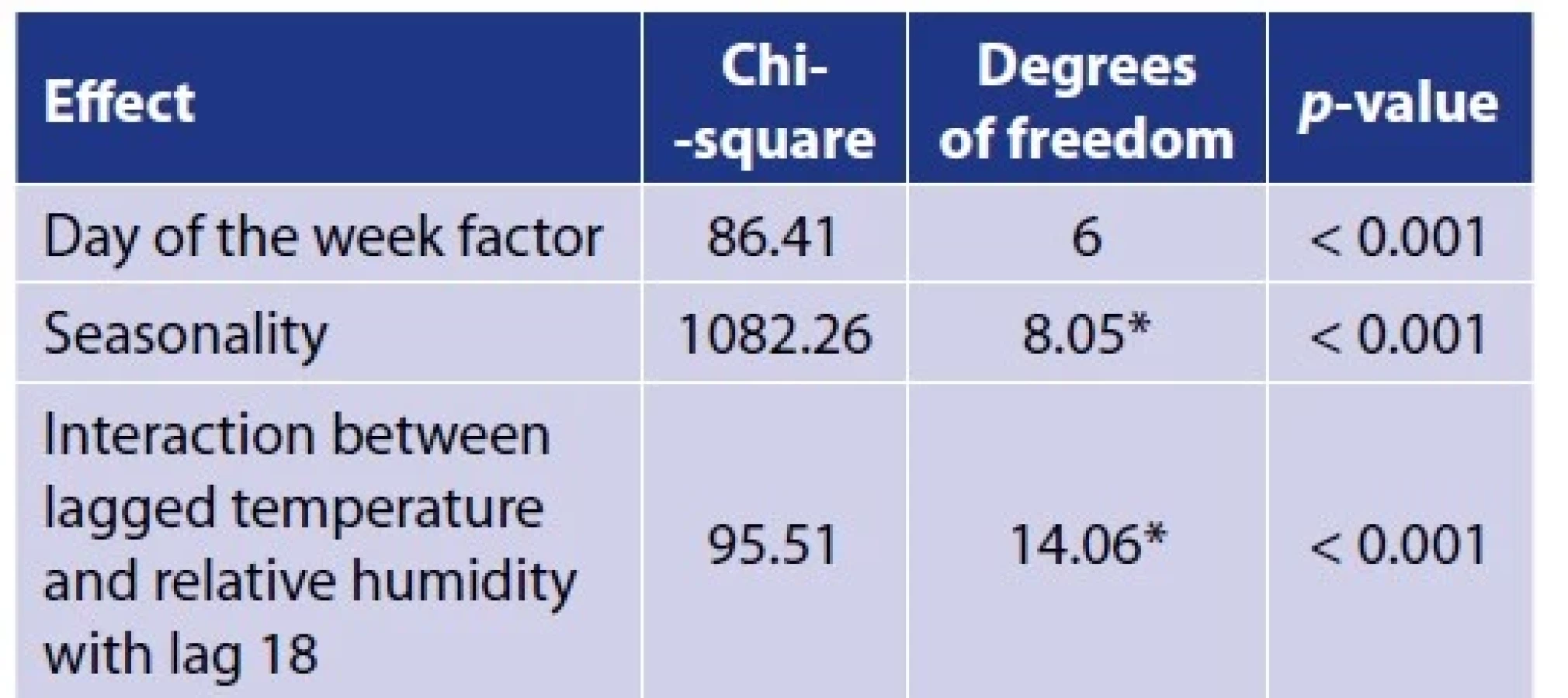

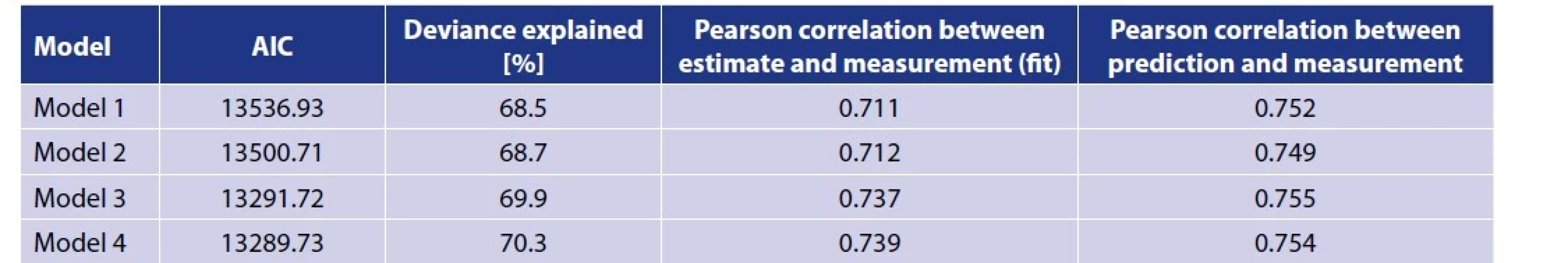
Figure 3 characterizes the average daily incidence of TBE depending on the interaction of meteorological conditions, i.e. temperature and relative air humidity at the time of infection of individual patients. The relevant values of the average daytime temperature and the interacting relative air humidity can be subtracted on both axes for each point on the graph area. The highest incidence is shown by a light yellow color, and the transition through the darker yellow to the orange and then red color corresponds to a decreasing incidence. White lines are isoline values of TBE incidence in the depicted meteorological situations of concurrent action of the two factors – that is, formally their interaction in the statistical sense. In other words, humidity modifies the effect of temperature, or even, equivalently, temperature modifies the effect of humidity. The highest TBE incidence are found in the area of a combination of high average temperatures (around 20 °C) and high relative air humidity (around 90%) at the top right of the chart. This meteorological situation, which determines the highest risk of appearance of new TBE clinical cases, may occur mainly during the peak summer. In some years it also occurs in late summer and this then conditions (or influences) the emergence and level of the second peak of the seasonal occurrence of TBE. In general, the graph shows the increasing demand for higher relative humidity with an increase in the average daily air temperature to maintain high incidence and therefore a high risk of infection. The graph also clearly shows a secondary area of relatively high intensities corresponding to average temperatures around 15 °C) and low relative air humidity (around 50%). The range of values on both axis of the graph is selected so that all combinations of daily averages of temperature and relative air humidity can be displayed continuously recorded throughout the reference time 2001–2015.

3.2.2 Model 2: Simple model with lag 18 and time-varying coefficient of interaction term between lagged temperature and relative humidity
The interpretation of Model 1 and the experience of long-term registration of the seasonality of clinical cases of KE warrant the assumption that the concomitant effect of Tavg and RH on the occurrence of cases of this disease shows certain seasonal changes.
In order to localise the results of Model 1 within the season of occurrence of new clinical cases of TBE, this model has been generalised to allow for a time-varying coefficient of the interaction term between temperature and relative humidity, both lagged by 18 days. A comparison of the individual models through AIC (see Table 2) suggests that Model 2 better explains the variability in the data. As a result, it is found that the time-changing coefficient shows a nonlinear course within the year, as demonstrated in Figure 4. In the period before the middle of the year (around the time of the 22nd calendar week), the value of the coefficient decreases as if there had been a temporary reduction in the influence of Tavg and RH on the TBE incidence. The nature and significance of the reduction in the value of the time-varying coefficient around the 22nd calendar week, which is concordant with knowledge of the predominantly bimodal seasonal course of TBE incidence, are analysed in the Discussion.

3.2.3 Model 3: Almon model trained on lag 18 and seasonality
To verify the results of a simple single-lag model, an Almon-based model has been developed that works with multiple lags simultaneously. For individual lags, the weights with which they contribute to the estimate are estimated. This approach makes it possible to deal with the problem of uncertainty in the search for a single resulting lag mentioned in the Model 1 in connection with Figure 1. Figure 5 shows the values of the weighing function with the appropriate point 95% confidence interval. The highest weight corresponds to lag 19 and the second secondary maximum is reached at lag 6. Model 3 provides some improvement in the deviance explained compared to the previous two models (Table 2), but this characteristic is satisfactory for all models compared.

3.2.4 Model 4: Almon model with time-varying coefficients trained on lag 18 and seasonality
As with the simple model described above, the Almon model was extended by time-varying coefficients in the next procedure. The resulting Model 4 has a lower AIC than Model 3 (see Table 2), but only by about 2. These models can therefore be assessed as virtually equivalent in terms of their ability to explain the variability in the observed data. A very small improvement in AIC does not offset a substantial increase in model complexity. As a result, we prefer a more parsimonious model, i.e. Model 3. Both models based on the Almon multi-lag approach have a slightly higher correlation between the estimate in each year and the actual number of registered cases than Models 1 and 2 with single lag (see Table 2).
3.3 The possibility to use the results obtained to clarify the prediction of the risk of clinical cases of TBE
The models described above, the parameters of which were estimated on the basis of input data from 2001 to 2015, were applied to similar data from the following year 2016, which was not used in modelling. This simulated, for demonstration purposes, the prediction of the epidemiological situation, i.e. the occurrence of new clinical diseases TBE after 18 days from the detected meteorological situation. The ability to predict is the most important criterion from a practical point of view. The best result from this point of view, i.e. the highest correlation of prediction with actually registered cases, was achieved, albeit by a little, model 3 (see Table 2). The result of the simulated prediction of this most successful model is demonstrated on Figure 6.

4 DISCUSSION
Regarding the dynamics of the TBE virus circulation in nature, and thus the level of risk of infection for occasional visitors to habitats with infected IR, the influence of climatic factors is most strongly mediated by the action on the vector organism - ticks. IR is qualified as an external (exophilic) species of a tick. This means that it is in direct contact with the host only at the time of blood sucking [31]. There are two ways to influence: short-term influences (in the order of hours or individual days), affecting mainly physical activity and causing, e.g. diurnal changes of location during the host-questing phase, and long-term influences (in the order of several days or weeks) affecting ontogenetic development, all physiological processes of ticks, diapauses (behavioural or developmental) as well as the replication of the TBEV in its body.
Attachment of a TBE-infected tick and at least short-term blood sucking is the main way humans are infected. Alimentary infections following the consumption of uncooked milk from lactating animals, especially goats and sheep infected with the TBEV, account for only a negligible fraction of the registered cases of TBE. However, clinical manifestations do not always occur. It is estimated that up to two thirds of people undergo TBEV infection without clinical signs, and the result is only the formation of antibodies [32]. In symptomatic patients, the course usually has two phases. In the first phase, fever and flu-like symptoms occur. After a short asymptomatic period, the second phase begins with a damage to the central nervous system. Exceptionally, in some patients, only the first phase may take place. The onset of various forms of clinical manifestations is associated with the overall health of the patient, his age, etc. However, the inapparent course, when only seroconversion occurred, may also indicate that during sucking only a lower dose of TBEV was transmitted than is the human clinical disease threshold.
Determining the influence of meteorological factors on the incidence of new cases of clinical disease TBE is conditioned by determining the time when the virus was transmitted: the tick was then active and physiologically ready to attack the host and at the same time the virus load in its body was high enough to be injected a dose of virus sufficient to exceeds the host infection threshold. In this work, this time is estimated through a lagged effect. This time interval includes in particular incubation period of the clinical TBE disease, which has been reported in medical practice as individually highly variable (2–21 days) due to the two-phase mode of the disease [15, 33, 34]. The observed lag values of L = 18 or L = 4 in this study (Model 1) may reflect different stages of the disease in which the infection is recognized and registered based on the first symptoms. Lag 18 appears to correspond to the onset of the neurological phase leading to hospitalization, while Lag 4 probably corresponds to the onset of influenza-like symptoms, which may not always manifest themselves and be noted. The situation is similar with L = 19 and L = 6 in Model 3. This confirms that the date of the first symptoms recorded in the routinely collected data is a mixture of the two mentioned time intervals.
Figure 3 shows the interactions of two abiotic factors (Tavg and RH), including ranges of values corresponding to the off-vegetation season. The observed characteristic (incidence of clinical cases of TBE) contains a significant biotic component – the activity of ticks infected with TBE virus. Its character, as verified in previous publications [15, 23, 31] is limited by ambient temperature: movement activity and host-questing activity take place to some extent above freezing point, and full physiological activity occurs above +10 °C. In laboratory experiments, Sixl and Nosek [35] paid attention to changes in the locomotor activity of all developmental stages of IR at both decreasing and rising ambient temperatures. They classified the observed tick reactions into 12 degrees from lethargy to escape reaction. For both nymphs and imagoes IR, the upper limit of normal activity was defined by stress, followed by increased activity leading to escape reaction. While the full normal activity of the imagoes IR was 18–25 °C, IR nymphs were normally active in the range of 10.0–22.5 °C (in both cases at 100% RH). This is consistent with our field findings [31]. During the six-year monitoring of IR activity, the spring-summer (higher) peak of the activity curve corresponded to habitat temperatures in the range of 10.1–15.0 °C, the summer-autumn (lower) peak in the range of 15.1–20.0 °C (or even more). The detected maximum temperature was 26.6 °C. This fact must be respected in the interpretation of the Figure 3, because used statistical model states in area of negative average temperature even very minimal but non-zero values of the incidence of new cases of TBE, which must be distinguished from the actually observed values. The area of the graph documenting the real natural conditions of the rise of clinical cases of TBE is thus, with regard to the occurrence of registered cases, limited from the point of view of the average daily temperature by a minimum of 0 °C and a maximum of 25 °C.
In the zone of average daily temperatures 0–10 °C, where the incidence of new clinical cases is very low, Tavg appears to be the decisive factor, rather than the interacting average air humidity (40% RH and above in the field shown in the graph). Isolines indicating sporadic occurrence of clinical cases of TBE thus occur at identical Tavg values across all RH values. This situation varies between 10–15 °C, when the interaction of Tavg and RH shows an increased effect of RH, which culminates in temperatures of 20 °C and higher. While the co-occurrence of high Tavg and RH values, corresponding to the high level of the incidence of new clinical cases of TBE can be seasonally localized to peak summer, possibly early autumn, the interaction of low Tavg with a relatively broad spectrum of RH can occur repeatedly in both the early spring and late autumn period. This supports the idea of how this result is affected by the fact that standard meteorological data are used as input data professionally measured at a height of 2 m. Humidity of the surface air level is strongly influenced by soil moisture, which is mostly high in spring after spring thawing of snow and frequent rains, while in summer the microclimate in the ground air layer is often affected by late summer soil moisture deficit and is therefore more dependent on the overall level of macroclimate humidity. This consideration should be taken into account when estimating the danger of attack by TBEV-infected ticks.
Regarding the results of model 2 with time-varying coefficients (see Figure 4), it should be noted that one of the basic features of the epidemiology of clinical human TBE cases is their seasonal occurrence, which in most cases is described by a bimodal curve. The first (and higher) peak is usually reached in late spring and early summer. During this period, the curve in the risk areas of TBE is very similar every year in terms of the shape and reaching values. In the next period, there is a temporary decline in the incidence of new cases, after which the subsequent re-increase in the number of new TBE culminates in a second, usually lower peak during the peak summer and early autumn. This second part of the seasonal curve is mostly subject to year-on-year differences. In extreme cases, the second peak is not created at all, or on the contrary reaches (or exceeds) the value of the spring-summer peak. The prevailing meteorological situation plays a significant role.
The biology of IR, the main vector of the TBE virus in Europe, is a driving factor in the virus circulation in nature. It also plays an important role in the epidemiology of human clinical diseases with this virus. The described course of TBE seasonality therefore largely corresponds to the curve of host-questing activity of IR. However, it is necessary to satisfactorily explain the different course of both curves in the second half of the growing season, when the second peak of TBE may exceed the spring values without a sudden increase in the number of host-questing active ticks. Such a case in the period under review was, for example, the year 2006, which, in addition to the extraordinary summer incidence of new TBE cases, was also extraordinary in terms of the summer meteorological situation. Further examples of similar annual courses are given in [23].
In 2001–2006, we performed a detailed study of host-questing IR activity depending on the meteorological conditions of the tick microhabitat [31]. Comparing the achieved data with the results of our previous study monitoring the population dynamics of IR in a long-term field experiment [36] we came to the conclusion that in the climate conditions of Central Europe the change of the structure of IR-active populations occurs in the period 22–23 calendar week. Most individuals (all stages) that successfully hibernated, have already found their host, and are either in a parasitic phase of life, or undergoing varying degrees of metamorphosis after sucking blood, and have disappeared from a cohort of host-questing active individuals. They are gradually replaced by freshly metamorphosed individuals who participate in the TBEV circulation, with their physiologically younger organisms being more susceptible to the virus than hibernating individuals [15]. Moreover, in this part of the season, the weather is characterized mainly by higher ambient temperature, so it depends mainly on the humidity of the air to what extent favourable conditions for the existence of IR occur. It is not just a host-seeking activity, but all the physiological processes in the tick and also the replication of the TBEV in its body. We analyzed these problems in detail in [15]. We hypothesized that elevated ambient temperatures in the second half of summer, accompanied by appropriate relative humidity, could cause intense replication of the TBEV in ticks, so that when people are attacked and their blood is sucked, they are more likely to be transmitted with a larger amount of TBEV exceeding the threshold for human infection with this virus. In this way, the risk of developing clinical diseases in infected people increases, which is also confirmed by the evidence that the risk of hospitalization for TBE increases during the year until August [37]. This also explains the regularly observed difference between the spring ratio of host-questing IR numbers and the number of established TBE clinical diseases compared with the second part of the summer, when the ratio is clearly higher in favour of new infections. At the same time, it supports the consideration of the influence of meteorological factors (and especially the interaction of Tavg and RH) influencing the epidemiological situation of TBE in this period of the year, important for predicting the risk of human infection with this virus. In Figure 3, the secondary area of relatively high incidence of TBE at average temperatures around 15 °C probably corresponds to the cases from late summer and early autumn.
Several authors, such as [38] created a predictive model in which predicted TBE rate increased with the increase of air temperature over the previous 10–20 days, precipitation over the previous 20–30 days, and forest characteristics (forestation, forest road density). In the case of the presented work, we used data on relative air humidity (% RH), which we consider more relevant. Summer precipitation in this period, which is mostly torrential and transient, has a strongly locally limited character. Their effects cannot be generalized to a wider area, as required by the nature of the TBE epidemiological input data, which is also necessary to make effective warning prognoses of the risk of the TBEV infection targeted by our research.
The incidence of TBE cases in 2016, which was used as the basis for the simulated “forecast“ because it was directly related to the previous fifteen-year analysis period, differed from previous years in the increased year-round incidence of TBE (565 cases). The seasonal course was also different, especially in its summer-autumn part, when the increased summer values of the occurrence followed (without a regular transient decrease) directly to the spring part of the curve, so that the second summer-autumn peak did not form markedly. The described situation corresponds to the findings in the pan-European area of TBE expansion [39]. This global difference from previous years therefore cannot be explained by the influence of some locally acting factors and remains unexplained. In detail, in the Czech Republic in October 2016 the seasonal incidence curve of TBE fell, but it partially increased during November (see Figure 6). This atypical situation probably reduces to some the quality of risk prediction by the model used, but on the other hand it shows that the model performs satisfactorily even under these circumstances. However, it should be acknowledged that the quality of the forecast may vary for different periods.
For effective real-time prediction of the risk of TBEV infection, it is not sufficient to use only weather forecast conditions, which generally enables human infestation by the IR tick. At the same time, the meteorological conditions must be respected, allowing the situation where an infected tick contains such an amount of virus that, when attacked a human, it transmits a dose of the virus that causes clinical disease.
Based on Figure 6, it can be stated that estimating the influence of the meteorological situation due to the interaction of Tavg and RH at the time of infection by TBEV (i.e. at the time of the biting by the infected tick) on the level of risk of clinical disease development (model 3) can be recommended as a basis for successful warning forecasts and a possible complement to forecasts based on host-questing tick activities.
5 CONCLUSIONS AND OVERLOOK
The aim of this study was to find out what is the relationship between the newly emerging cases of clinical TBE disease as a dependent variable and various predictors, especially the average daily temperature and average relative air humidity and their interaction. It is a matter of determining the meteorological conditions under which the host-questing stage of IR was physiologically prepared to attack the host, suck its blood, and the TBEV load in the IR vector was high enough to deliver a dose of virus exceeding the human infection threshold and thus to cause human clinical disease. The methodological benefit is that a model with quantitatively characterized effects of temperature, air humidity and their interaction is used for this purpose, which works with the delay of the effect estimated through the optimization process.
All cases of TBE in the Czech database of infectious diseases EpiDat, which is the initial source of data for the performed analyzes, are time-localized according to the date of detection of the first clinical symptoms. Based on these data, a time estimate is based on when the affected person was infected with an IR tick, which is a necessary first step in monitoring the influence of meteorological factors determining the development of clinical TBE. The estimated time between the infestation of a human by an infected IR tick and the onset of the first symptoms corresponds to a large extent to the term incubation period of the disease used in clinical practice, but the calculation is not its net value. It can be burdened both by the subjective perception of patients and by the nature of the data coming from the routine surveillance system. In addition, TBE usually has a two-phase course and may be a mixture of two time ranges in determining the first symptoms. From a statistical point of view, the modelling of the time at which an affected person has been infected with tick is an assessment of the delayed effect/lag, and this designation is used in all models. The resulting value of lag L = 18 (delay of the effect by 18 days) used in further analyzes was selected based on the comparison of models with different lags.
The basic model used relates the occurrence of TBE to the interaction of ambient temperature and relative air humidity with above mentioned shift, and it also includes the effect of the season and the effect of the day of the week. Other models consider and compare the possibility of using alternative lags, including models based on the Almon approach, which work with multiple lags at the same time. The relationship between the two meteorological factors and their interactions changes during the season of host-questing IR activity, and with it the conditions for the occurrence of new clinical cases of TBE change, as summarized graphically in Figure 3.
The results and their interpretations follow the studies [23] and [15]. In addition, the prognosis of the risk of IR tick attack will focus specifically on predicting the risk of acquiring clinical TBE in real time. The presented results can also be used to estimate the penetration of this serious neuroinfection into new geographical areas, which will allow the expected future global climate change.
Acknowledgement
The study was supported by the Czech Science Foundation, project 22-24920S.
Do redakce došlo dne 12. 12. 2022.
Adresa pro korespondenci
RNDr. Marek Malý, CSc.
Státní zdravotní ústav
Šrobárova 49/48
100 00 Praha 10
e-mail: marek.maly@szu.cz
Sources
1. Lindquist L, Vapalahti O. Tick-borne encephalitis. Lancet, 2008;371:1861–1871.
2. Beauté J, Spiteri G, Warns-Petit E, et al. Tick-borne encephalitis in Europe, 2012 to 2016. Euro Surveill., 2018;23(45):1800201.
3. Orlíková H, Vlčková I, Manďáková Z, Kynčl J. Tick-borne encephalitis in the Czech Republic in 2021. Zprávy Centra epidemiologie a mikrobiologie, 2022;31(8):308–318.
4. Jenkins VA, Silbernagl G, Baer LR, et al. The epidemiology of infectious diseases in Europe in 2020 versus 2017–2019 and the rise of tick-borne encephalitis (1995–2020). Ticks Tick-Borne Dis., 2022;13:101972.
5. Gray JS, Dautel H, Estrada-Peña A, et al. Effects of climate change on ticks and tick-borne diseases in Europe. Interdiscip Perspect Infect Dis., 2009;2009:593232.
6. Hubálek Z, Halouzka J, Juřicová Z. Host-seeking activity of ixodid ticks in relation to weather variables. J. Vector Ecol., 2003;28(2):159–165.
7. Korenberg EI. Seasonal population dynamics of Ixodes ticks and tick-borne encephalitis virus. Exp. Appl. Acarol., 2000;24:665–681.
8. Randolph SE. The impact of tick ecology on pathogen transmission dynamics. In: Bowman AS, Nuttall PA (Eds.). Ticks: Biology, Diseases and Control. Cambridge: Cambridge University Press;2008. pp. 40–72. ISBN 978-0-521-86761-0.
9. Sirotkin MB, Korenberg EI. Influence of abiotic factors on different developmental stages of the taiga tick Ixodes persulcatus and sheep tick Ixodes ricinus. Entomol. Review, 2018;98(4):379–396.
10. Danielová V, Daniel M. Climate, ticks and tick-borne encephalitis in Central Europe. In: Nuttall P (Ed.). Climate, Ticks and Disease. Wallingford: CAB International;2022. pp. 331–340. ISBN 978-1-78924-963-7.
11. Voyiatzaki C, Papailia SI, Venetikou MS, et al. Climate changes exacerbate the spread of Ixodes ricinus and the occurrence of Lyme borreliosis and tick-borne encephalitis in Europe – how climate models are used as a risk assessment approach for tick-borne diseases. Int. J. Environ. Res. Public Health, 2022;19:6516.
12. Menne B, Ebi KL (Eds.). Climate chase and adaptation strategies for human health. Darmstadt: Steinkopff Verlag;2006.
13. Daniel M, Vráblík T, Valter J, et al. The TICKPRO computer program for predicting Ixodes ricinus host-seeking activity and the warning system published on websites. Cent. Eur. J. Public Health, 2010;18:234–240.
14. Czech Hydrometeorological Institute. Ticks activity. [Accessed 2022-12-06]. Available at: https://info.chmi.cz/bio/mapy.php?type=kliste. [In Czech.]
15. Daniel M, Danielová V, Fialová A, et al. Increased relative risk of tick-borne encephalitis in warmer weather. Front Cell Infect. Microbiol., 2018;8:90.
16. Van Heuverswyn J, Hallmaier-Wacker LK, Beauté J, et al. Spatiotemporal spread of tick-borne encephalitis in the EU/EEA, 2012 to 2020. Euro Surveill., 2023;28(11):2200543.
17. Nuttall P (Ed.). Climate, ticks and disease. Wallingford: CAB International;2022. 566 pp. ISBN 978-1-78924-963-7.
18. Daniel M, Beneš Č, Danielová V, et al. Sixty years of research of tick-borne encephalitis--a basis of the current knowledge of the epidemiological situation in Central Europe. Epidemiol. Mikrobiol. Imunol., 2011;60(4):135–155.
19. Kunze M, Banović P, Bogovič P, et al. Recommendations to improve tick-borne encephalitis surveillance and vaccine uptake in Europe. Microorganisms, 2022;10(7):1283.
20. Prymula R. Prevention possibilities and vaccination against tick-borne encefalitis. In: Růžek D (Ed.). Klíšťová encefalitida [Ticks-borne encefalitis]. Prague: Grada Publishing House;2015. pp. 155–172. ISBN 978-80-247-5305-8.
19. Rawlings JO, Pantula SG, Dickey DA. Applied Regression Analysis: A Research Tool. 2nd ed. New York: Springer;1998. ISBN 978-0-387-98454-4.
20. Wood SN. Generalized Additive Models: An introduction with R. 2nd ed. Boca Raton: Chapman & Hall/CRC;2017. ISBN 978-1-498-72833-1.
21. Brabec M, Daniel M, Malý M, et al. Analysis of meteorological effects on the incidence of tick-borne encephalitis in the Czech Republic over a thirty-year period. Virol. Res. Rev., 2017;1(1):1–8.
22. Burnham KP, Anderson DR (Eds.). Model Selection and Multimodel Inference: A practical information-theoretic approach. 2nd ed. New York: Springer-Verlag;2002. ISBN 978-0-387-95364-9.
23. Hastie TJ, Tibshirani RJ. Generalized Additive Models. Boca Raton: Chapman & Hall/CRC;1990. ISBN 978-0-412-34390-2.
24. Hastie T, Tibshirani R. Varying-coefficient models. J. R. Statist. Soc. B, 1993;55(4):757–796.
25. Brabec M. Semiparametric model for short term effects of air pollution upon asthma symptoms exacerbations. Joint ISCB/ASC Meeting, Melbourne, Australia, August 26–30, 2018.
26. Judge GG, Griffiths WE, Hill RC, et al. The Theory and Practice of Econometrics. New York: Wiley;1980. ISBN 978-0-471-05938-7.
27. Almon S. The distributed lag between capital appropriations and net expenditures. Econometrica 1965;33:178–196.
28. R Core Team. R: a language and environment for statistical computing. R Foundation for Statistical Computing, Vienna, Austria. [Accessed 2022-06-10]. Available at: http://www.R-project.org/.
29. Daniel M, Malý M, Danielová V, et al. Abiotic predictors and annual seasonal dynamics of Ixodes ricinus, the major disease vector of Central Europe. Parasit Vectors, 2015;8:478.
30. Luňáčková J, Chmelík V, Šípová L, et al. Epidemiologické sledování klíšťové encefalitidy v jižních Čechách. Epidemiol. Mikrobiol. Imunol., 2003;52:51–58.
31. Duniewicz M. Central European Tick-borne encephalitis. In: Duniewicz M, Adam P. (Eds.). Neuroinfekce. Maxdorf: Prague;1999. pp. 119–127. ISBN 80-85800-72-1.
32. Penyevskaya NA. Methodological approach to the estimation of efficacy of etiotropic immunoprophylaxis in tick-borne encephalitis. Clin. Microbiol. Antimicrob. Chemother., 2008;10:70–84. [In Russian.]
33. Sixl W, Nosek J. Einfluss von Temperatur und Feuchtigkeit auf das Verhalten von Ixodes ricinus, Dermacentor marginatus, und Haemaphysalis inermis. Archives des Sciences, 1971;24(1): 97–109.
35. Daniel M, Dusbábek F. Micrometeorological and microhabitat factors affecting maintenance and dissemination of tick-borne diseases in the environment. In: Sonenshine DE, Mather TN (Eds.). Ecological Dynamics of Tick-Borne Zoonoses. Oxford: Oxford University Press;1994. pp. 91–138. ISBN 978-0-19-507313-3.
37. Borde JP, Kaier K, Hehn P, et al. Tick-borne encephalitis virus infections in Germany. Seasonality and in-year patterns. A retrospective analysis from 2001-2018. PLoS ONE, 2019;14(10): e0224044.
38. Stefanoff P, Rubikowska B, Bratkowski J, et al. A predictive model has identified tick-borne encephalitis high-risk areas in regions where no cases were reported previously, Poland, 1999–2012. Int. J. Environ. Res. Public Health, 2018;15(4):677.
39. European Centre for Disease Prevention and Control. Tick-borne encephalitis. In: Annual epidemiological report for 2016. Stockholm: ECDC;2018. [Accessed 2022-12-06]. Available at: https://www.ecdc.europa.eu/sites/portal/files/documents/AER_for_2016-TBE.pdf.
Labels
Hygiene and epidemiology Medical virology Clinical microbiologyArticle was published in
Epidemiology, Microbiology, Immunology

2023 Issue 2
Most read in this issue
- Selected aspects of mortality in Czechia and Slovakia in the pandemic year 2020
- A word on the microbiome: considerations about the history, current state, and terminology of an emerging discipline
- The influence of meteorological factors on the risk of tick-borne encephalitis infection
- Comparison of invasive and non-invasive isolates of Neisseria meningitidis by whole genome sequencing, Czech Republic, 2005–2021