
Face Recognition Algorithm Based on Fast Computation of Orthogonal Moments


1
Department of Computer Engineering, University of Baghdad, Al-Jadriya, Baghdad 10071, Iraq
2
Electrical Engineering, College of Engineering, University of Ha’il, Ha’il 682507, Saudi Arabia
3
Czech Academy of Sciences, Institute of Information Theory and Automation, Pod Vodárenskou vìží 4, 18208 Prague, Czech Republic
4
Faculty of Management, University of Economics, Jarosovska 1117/II, 37701 Jindrichuv Hradec, Czech Republic
*
Author to whom correspondence should be addressed.
†
These authors contributed equally to this work.
Mathematics 2022, 10(15), 2721; https://doi.org/10.3390/math10152721
Submission received: 11 June 2022
/
Revised: 26 July 2022
/
Accepted: 29 July 2022
/
Published: 1 August 2022
(This article belongs to the Special Issue Advances in Pattern Recognition and Image Analysis)
Abstract
:Face recognition is required in various applications, and major progress has been witnessed in this area. Many face recognition algorithms have been proposed thus far; however, achieving high recognition accuracy and low execution time remains a challenge. In this work, a new scheme for face recognition is presented using hybrid orthogonal polynomials to extract features. The embedded image kernel technique is used to decrease the complexity of feature extraction, then a support vector machine is adopted to classify these features. Moreover, a fast-overlapping block processing algorithm for feature extraction is used to reduce the computation time. Extensive evaluation of the proposed method was carried out on two different face image datasets, ORL and FEI. Different state-of-the-art face recognition methods were compared with the proposed method in order to evaluate its accuracy. We demonstrate that the proposed method achieves the highest recognition rate in different considered scenarios. Based on the obtained results, it can be seen that the proposed method is robust against noise and significantly outperforms previous approaches in terms of speed.
Keywords:
face recognition; orthogonal polynomials; orthogonal moments; feature extraction; block processingMSC:
68T45; 68U101. Introduction
Face recognition has been used in various fields, such as personal identification [1,2] descriptions of gender and gestures [3], victim identification, surveillance security systems, medical diagnosis, multimedia communication, and human–computer interfaces [4,5]. The face has different cues that help to uniquely identify an individual human. These cues have been widely utilized by authentication and verification algorithms to extract diverse discriminative features, achieving accurate identification [4,6]. The wide spectrum of facial features has enabled face recognition challenges to attract broad interest compared to other biometric systems, and it has become one of the most important topics of research [7,8,9]. In addition, the robustness of the face localization and normalization processes are considered the core of an efficient feature extraction process [10].
Even though many face recognition methods have been studied, system accuracy and processing time remain critical issues and need to be treated carefully. Generally, the results of well known methods do not provide the required accuracy with a fast execution time. Therefore, careful investigation of an accurate and fast face recognition method is required. Moreover, to the best of our knowledge, most of the existing works do not take into consideration the effect of noise in input images. Noise may appear mainly in non-cooperative applications, where the lighting conditions are beyond control.
In order to address the above-mentioned challenges, the present paper proposes a robust face recognition algorithm by using a kind of Hybrid Orthogonal Polynomials (HOPs), specifically, Squared Krawtchouk–Tchebichef polynomials (SKTP) [11], and a fast overlapping block processing algorithm for feature extraction. These HOPs have been used widely in the literature on image and signal processing because of their powerful capabilities in feature extraction. In addition, the use of the fast algorithm for overlapping block processing [12] provides the construction of auxiliary matrices, which virtually extends the original image and makes it possible to avoid time-consuming computation loops. The introduced solution reaps the benefits of adopting the SKTP model in multiple dimensions. The energy compaction and localization properties of the SKTP outperform the existing orthogonal polynomials (OPs) and other hybrid-form OPs, which helps to represent the images efficiently and reduces the computation cost of feature extraction. In addition, the extraction of moments from overlapped blocks increases the robustness of the features, which in turn increases the recognition rate. One of the main advantages of the proposed solution is its high robustness to noise in the input images. This is achieved by standard Gaussian smoothing implemented in a novel way: the Gaussian kernel is embedded into the moment calculation step, meaning that it does not increase the computation time.
1.1. Literature Review and Discussion
There are several well known classes of image feature extraction methods: deep learning methods, the eigenface and Fisher face methods, texture-based methods, and projection-based methods. This last approach “projects” facial images on a functional basis and uses these projection coefficients as features. The basis is usually formed by a set of orthogonal functions such as wavelets, harmonic functions or polynomials [2]. The method we propose in this paper falls into this category.
Deep learning-based approaches have a high level of recognition accuracy; however, they require a large amount of data to perform better than other methods and provide an extreme level of computational complexity [13,14,15,16,17]. In the OM-based methods, the features of faces can be computed effectively using Orthogonal Polynomials (OPs) [11]. In recent works, OPs and their moments have been intensively used for image analysis, shape descriptors, and pattern recognition [18]. In the moment domain, image components are represented in a transform domain, offering a powerful capability for analyzing them [11]. Orthogonal moments (OMs) can be defined as scalar quantities that are utilized to characterize the function and capture its significant features. In addition, they are the coordinates of an image in the orthogonal polynomial function [19,20]. Furthermore, OMs have the ability to extract features from images that have different geometric invariants, such as translation, scaling, and rotation [2].
Different types of moments are used in image processing systems. First, geometric moments have been introduced over other kinds of moments due to their explicit geometric meaning and simplicity [21]. Zernike and Pseudo-Zernike moments are utilized to represent the image with minimal redundancy of information [22], while fractional quaternion Zernike moments have been used for detection of color image copy–move forgery [23] because fractional-order polynomials can represent functions better than integer-order polynomials [2]. Fractional-order Zernike moments have been used efficiently in plant disease recognition [24]. Legendre moments were used in [25] to reduce block artifacts. For image analysis, Zernike and Legendre polynomials are used as kernel functions for Zernike and Legendre moments, respectively [26]. In addition to the ability of Zernike moments to store information about images with minimum redundancy, they have the property of invariance. However, these moments require image coordinate transformations for discrete situations, as they are defined specifically in the continuous domain [27].
Recently, discrete orthogonal moments have been adopted to overcome the computational cost of image analysis of continuous moments [28]. Mukundan presented a set of moments to analyze the image using discrete Tchebichef polynomials [29]. In addition, Tchebyshev moments have been implemented in watermarking algorithms and image encryption algorithms [30]. For face recognition, an adaptively weighted patch of pseudo-Zernike moments has been used [31]. Different OMs have been used in this field, such as higher-order OMs [32], Fourier–Mellin moments [33], rotation-invariant complex Zernike moments [34], discrete Krawtchouk moments [35], Tchebichef moments [36], orthogonal exponent Fourier moments [37], 2D orthogonal Gaussian–Hermite moments [38], and 2D Krawtchouk moments [21]. The 2D Krawtchouk OMs provided good results in conditions with noise, tilt, and changes in expression [39]. In comparison with other moments, Gaussian–Hermite moments are considered very robust against noise [28,40]. Gaussian–Hermite moments can bne used as a set of useful features to capture the facial expression from face images [39,41]. Generally, the extraction methods of image features are classified into two groups: global features-based methods (termed Holistic approaches [42]) and local features-based methods (termed Component-based methods [42] or Block Processing-based methods). The former method captures the features from an entire image of a human face, while the local feature extraction method can extract features from certain areas of the face image, such as the eyes, mouth, and chin [39]. There are various global feature extraction methods, such as Eigenfaces [43], Fisher faces [44], Linear Discriminant Analysis [45], Discrete Cosine Transform [46], Independent Component Analysis [47], and others. The global features-based method has achieved superior performance when implemented with different imaging conditions [48].
In block processing-based methods the extraction of image features can be performed locally using OMs, meaning that processing of the image blocks takes place after partitioning. Block processing is implemented in different applications of signal processing in which signals (images and videos) are partitioned into blocks. These blocks are converted to the transform domain in order to extract the features, which are stored in a memory location equivalent to the image block for processing in the next steps [12]. In general, block processing-based methods perform better than holistic-based methods [42]. Local Binary Patterns is one of local feature extraction methods, it is used to partition face image into sub-images where feature distribution is extracted and fused together [49]. This method is a good descriptor to represent local structures [50,51]. A combination of global and local methods, that is called a Fusion (or hybrid) algorithm, is also adopted to achieve a desired face recognition with high accuracy [39,48].
Block processing that represents local feature extraction provides high accuracy at the expense of increased computation cost. Different types of transforms have been used for this purpose. Gabor transform [52] has been used widely to extract the local features [53,54], alhough the extracted face features are particularly sensitive to noise. In addition, face recognition methods that use local feature are dependent on face localization and the registration model [39]. In [55], an algorithm for face recognition was proposed in which Krawtchouk polynomials with different values of parameters were used for noise-free and noisy environments. This algorithm can overcome the problem of numerical instability by utilizing symmetry properties across polynomials’ diagonals to address the effect of their parameter on feature extraction. The computation cost of this method is considered relatively high. Partitioning of the images using image block processing extracts the blocks of the images and processes them sequentially. This process is not sequential from the perspective of the memory, however, which is considered a key drawback in terms of computation performance and results in an essential gap between CPU speed and memory. Accessing the entire matrix in sequence maintains the spatial locality, although it causes more cache misses and replacements [12]. Exclusion of further processes accelerates the extraction of local features; in other words, the extraction of local features from the image blocks by discrete transformation decreases computational complexity. This is called the fast overlapping block processing algorithm [12].
1.2. Contributions
The main contributions of this paper are: (1) design of a robust face recognition method for multiple imaging conditions following the shape-invariant concept; (2) use of powerful hybrid OPs called SKTP to extract image features; (3) utilization of a fast-overlapping block processing algorithm for feature extraction in order to decrease computation time; and (4) application of an embedded filter to suppress noise and maintain the speed of feature extraction.
2. Preliminaries of Orthogonal Polynomials and Moments
In this section, the mathematical model of the utilized orthogonal polynomials and the computation of their moments for two-dimensional signals are presented.
2.1. Squared Krawtchouk–Tchebichef Polynomials
The concept of discrete orthogonal polynomials is to project a signal on the orthogonal polynomial basis. In image analysis, we consider 2D signals. Discrete orthogonal polynomials are used to describe the signal efficiently and without redundancy [56]. Discrete orthogonal polynomials are defined using two variables (x and n), forming a two-dimensional matrix. The variable x represents the index (coordinate) of the signal, and the variable n represents the order of the polynomial. The coefficients of the matrix are the values of the discrete orthogonal polynomials. In this paper, Squared Krawtchouk—Tchebichef Polynomials (SKTP) and their moments are used. SKTPs are formed from the combination of the Krawtchouk polynomials (KPs) and Tchebichef polynomials (TPs). This combination results in a polynomial with the properties of both KP and TP, i.e., an SKTP shows localization and energy compaction compared to other types of polynomials [57]. Thus, SKTPs leverage the accuracy of face recognition. The nth order of the SKTP is defined in terms of KP (K) and TP (T) for as follows [11]:
where p represents the polynomial parameter. The definition of SKTP can be written in matrix form as follows:
where and represent the matrices of the KP and TP.
Orthogonal polynomials can be efficiently calculated by recurrent relations, which is a way that is fast and prevents precision loss due to overflow/underflow. The algorithms used for evaluation of KP and TP in this paper are provided in Appendix A.
2.2. Squared Krawtchouk–Tchebichef Moments
It is well known that the discrete moments are considered essential tools in different applications [19,58]. Specifically, the discrete moments are used for signal representation due to their being, at least to an extent, robust to noise effects [59]. In addition, the moments are scalar quantities and as such are able to reveal the small changes that appear in signals [60]. For these reasons, discrete moments are utilized in face recognition. As mentioned earlier, the discrete moments are scalar quantities, and are produced for a 1D signal from the projection of the signal onto the discrete orthogonal polynomial basis functions. In addition, they can be produced for 2D signals (images) from the projection of the images on the discrete orthogonal polynomials’ basis images [56]. In this paper, Squared Krawtchouk–Tchebichef moments (SKTM) are used, and are computed as follows:
Generally, discrete moments represent the descriptors (features) in two folds: the low-order moments and the high-order moments. The low-order moments preserve the signal information, while the high-order moments represent the details of the signal [60]. Thus, for feature extraction, the low order moments ( and ) need to be utilized as follows:
The moments are computed using matrix multiplication as
where represents the matrix transpose.
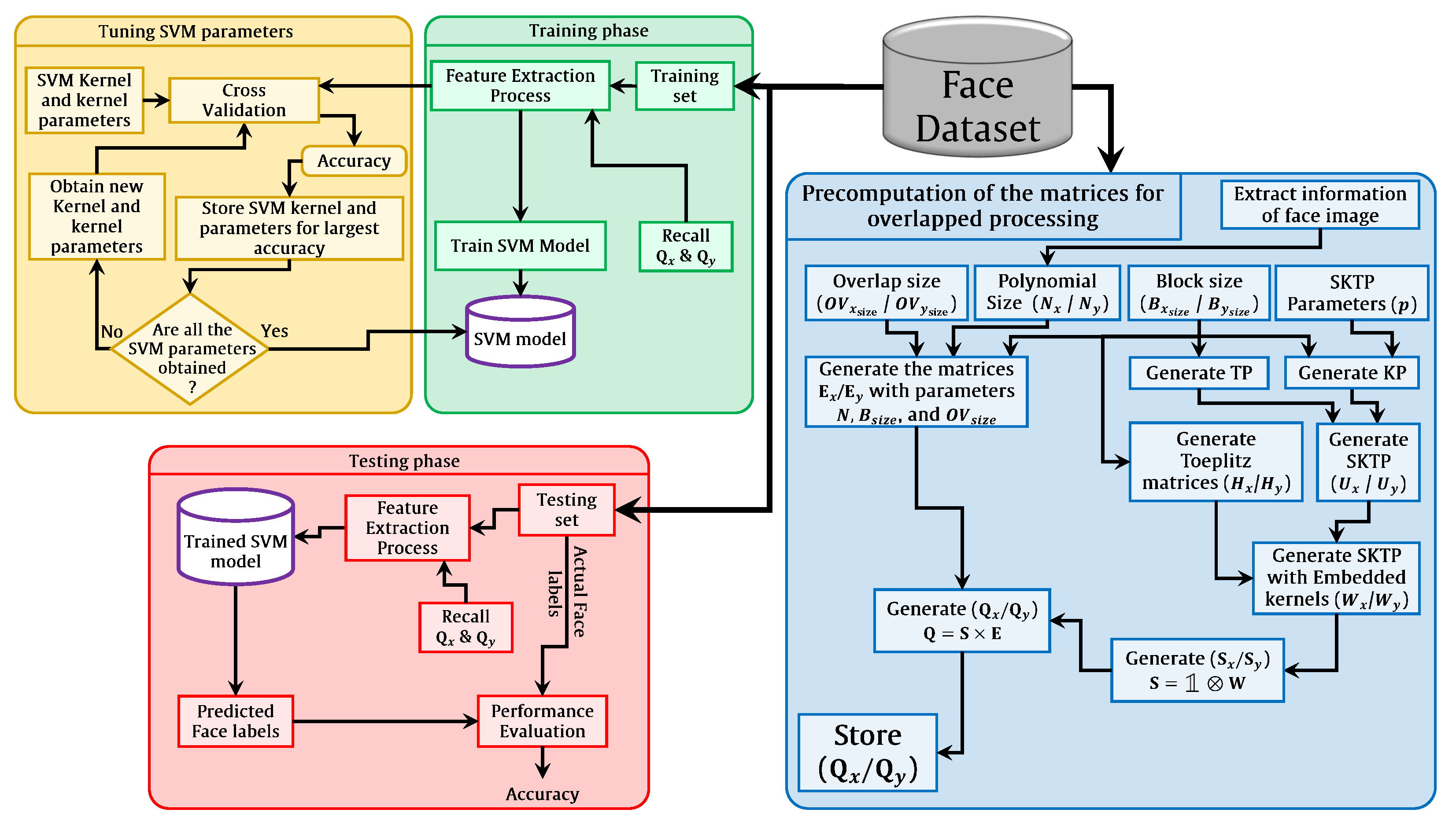
3. Methodology
In this section, the feature extraction process and the recognition process for face recognition are described. The flowchart of the proposed face recognition method is shown in Figure 1.
The feature extraction process is the main part of any recognition system. For the sake of accurate results, instead of using a global feature, local feature extraction is used to enable more efficient face recognition. Local features are considered more robust and leverage the recognition accuracy when compared to global features [61,62,63]. Therefore, in order to increase the robustness of recognition accuracy, the face image is partitioned into blocks with a block size of . The TP and KP are generated using the procedures in Appendices Appendix A.1 and Appendix A.2, respectively. Note that the KP is generated with a localization parameter p. After obtaining the two matrices of KP and TP, the SKTP matrices ( / ) are generated using Equation (2).
Most face recognition algorithms have concentrated on a collaborative scenario in a noise-free environment. In a noisy environment, the face recognition process is degraded and the face recognition accuracy is significantly affected. Thus, face image preprocessing is needed to reduce the noise effect without excessively increasing the computation cost. The use of embedded image kernels to reduce computation cost was proposed in [64], and we adopt this idea here. In order to embed a smoothing kernel in the generated SKTP matrices ( / ), Toeplitz matrices ( / ) are generated [65] using a Gaussian smoothing kernel:
where determines the effective size of the kernel (most often ). Thus, ( / ) can be generated as follows [65]:
where m and l are the lengths of the smoothing kernels and , respectively. To this end, the embedded SKTP matrices ( / ) can be formulated as follows [64]:
After generating the SKTP matrices with embedded smoothing kernels, we are ready for the feature extraction step. However, the use of traditional methods to extract local features leads to a high computation cost [66], as they extract the local features directly from the small blocks. Most applications utilize non-overlapped block processing to extract local features. However, overlapped block processing increases the recognition accuracy [67,68,69]. Thus, in this paper, overlapped block processing is performed. It is well known that overlapped block processing increases the computation cost considerably. In order to overcome this problem, we utilize the fast overlapped block processing method presented in [12]. The main concept of fast overlapped block processing (FOBP) is based on the creation of auxiliary matrices that extend the image and eliminate the need for a nested loop. The elimination of the nested loops greatly reduces the computation cost of the feature extraction process.
Suppose an image has rows and columns. The image is partitioned into overlapped blocks with a size of , with overlap size in the x-direction and in the y-direction such that the total blocks are equal to . Suppose the matrix represents the extended image version of ; it can be generated as follows [12]:
where and are rectangular matrices with a size of and , respectively. For further elucidation, the matrix is provided by
![Mathematics 10 02721 i001]() where represents the identity matrix, with a size of . Now, the moments for the overlapped block can be computed as follows:
where and . To obtain the matrices and , they can be formulated as follows [12]:
where ⊗ represents the Kronecker product and represents the identity matrix. Because these matrices are independent of the image, they are computed first, stored, and utilized repeatedly [12].
where represents the identity matrix, with a size of . Now, the moments for the overlapped block can be computed as follows:
where and . To obtain the matrices and , they can be formulated as follows [12]:
where ⊗ represents the Kronecker product and represents the identity matrix. Because these matrices are independent of the image, they are computed first, stored, and utilized repeatedly [12].

After generating the required matrices ( and ), the images are sent to the next stage for feature extraction and classification. Note that the extracted features are normalized.
After the normalized feature vector has been obtained, a label (ID) is applied to each input face image. The feature vector is considered as an input to the classifier. The classification itself is performed by a support vector machine (SVM) classifier. The SVM approach was chosen because of its ability to optimize the margin between two hyperplanes separating the classes [70]. In addition, SVM is suitable for recognition, as it is more robust to signal fluctuation than nearest-neighbor classifiers [71]. In this paper, LIB-SVM was applied [72].
4. Experiments and Analysis
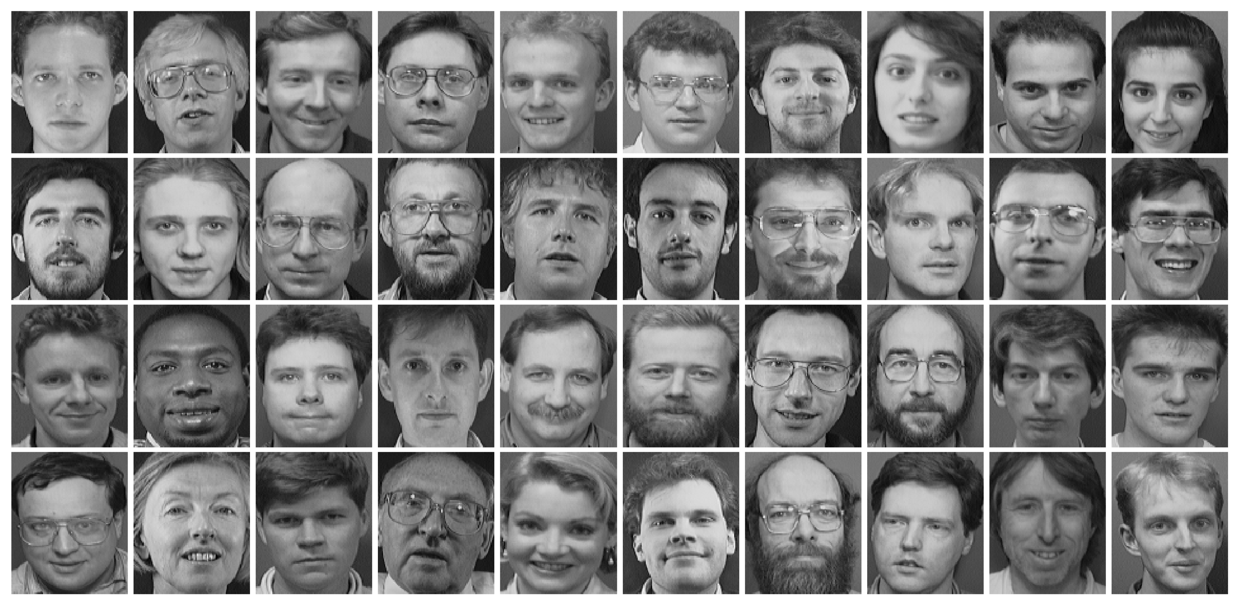
In this section, two different datasets are employed to evaluate the performance of the face recognition algorithm. The datasets used in the experiments are the ORL [73] and FEI datasets [74]. The ORL Face Database from AT&T [73] is a well-known datset which has been used by many researchers for evaluation purposes. The ORL dataset includes 40 distinct classes (persons). Each class has ten images, which are acquired at different position and lighting conditions to form 400 images, and each image has a size of [75]. Figure 2 shows samples of the ORL face dataset.
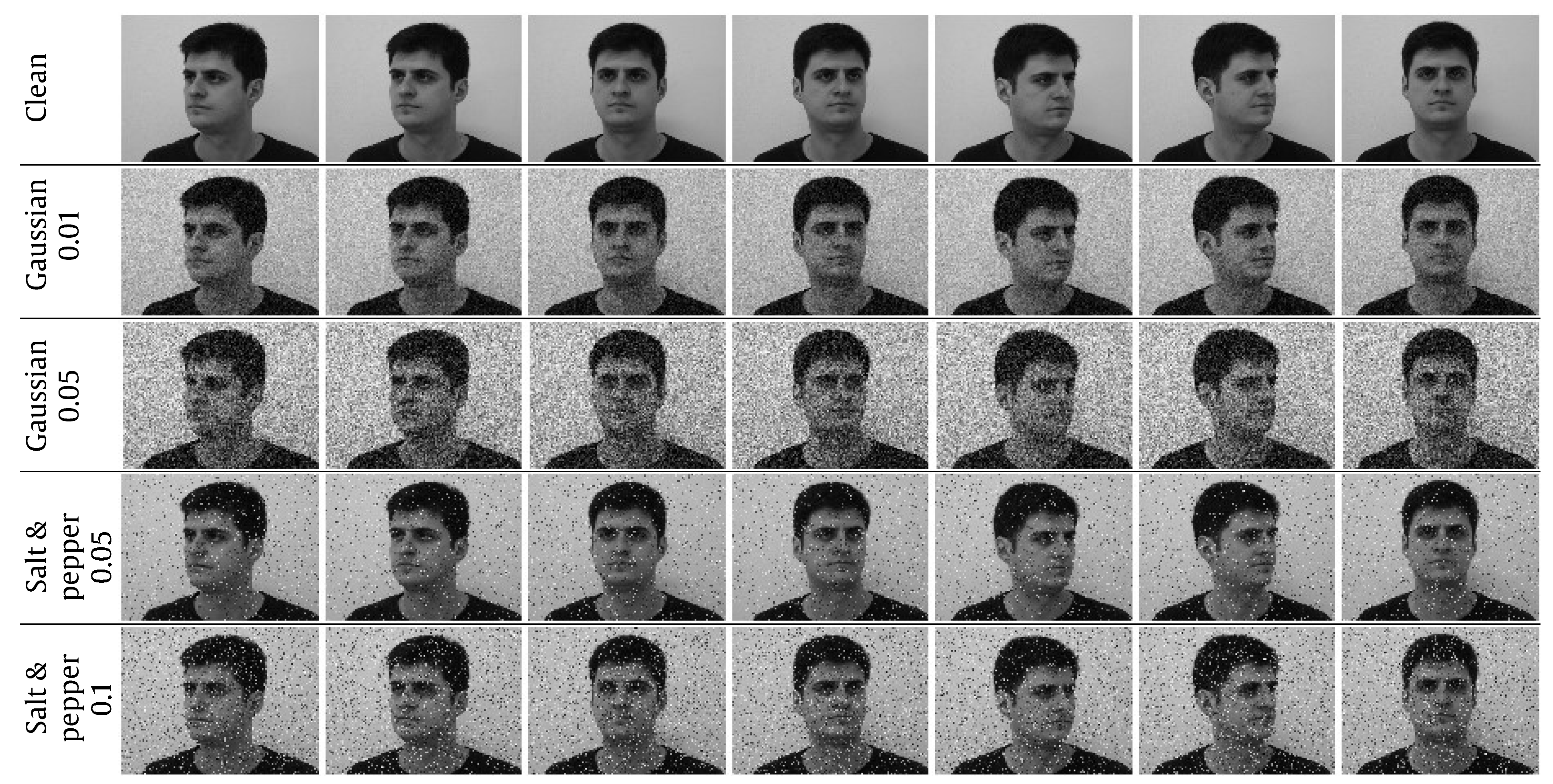
For the ORL dataset, the block size in the x and y directions was set to 16 and 20, respectively. The overlap sizes in the x and y directions were set to {(0,0), (2,2), (4,4), (8,8)}. The size of the smoothing kernel was set to {3, 5, 7}. In addition, the test was performed with noise-free and noisy environments and with Gaussian and Salt and Pepper noise. The Gaussian noise was generated with the standard deviation 0.005, and 0.01, respectively. The Salt and Pepper noise was generated with densities 0.05 and 0.1. Figure 3 depicts samples of images with different types of noise. Table 1 summarizes the average results for 20 runs, and the detailed results of individual runs can be found in Appendix B.
For SVM implementation, we used LIB-SVM [72]. In the training phase, five-fold cross-validation was employed to obtain stable values of the SVM parameters.
First, an experiment was carried out for the proposed algorithm using two cases, with and without a smoothing kernel. This experiment was performed to highlight the effect of the smoothing kernel on the recognition accuracy. The experiment was performed for different overlap sizes of {(0,0), (2,2), (4,4)} and different environments (noise-free and noisy environments), as shown in Table 2. Note that the results reported in Table 2 represent the average results for 20 runs; the detailed results of individual runs can be found in Appendix C. The results show that the recognition accuracy of the proposed algorithm is higher with a smoothing kernel than that without, with average recognition accuracy showing an improvement ratio of ∼0.5%.
Another experiment was performed to identify the best block overlap size and smoothing parameter , which determines the kernel size (the kernel size was always taken as to maintain more than 95% of the ideal Gaussian filter). The optimal of course depends on the noise level and on the images themselves; in our case, we conclude that is the best choice, providing the highest recognition performance (see Table 1). As for the block overlap, it can be observed that while the differences are slight, the overlap (4,4) mostly yields the best results.
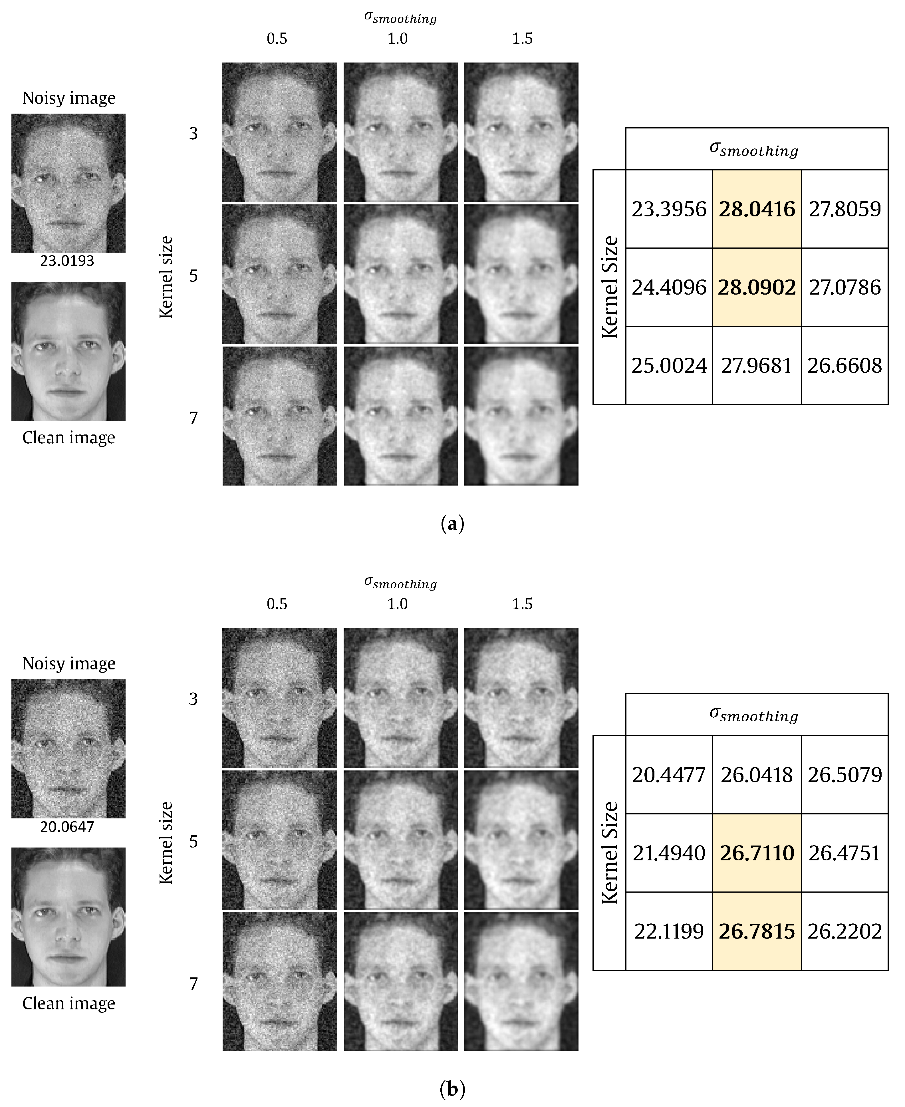
The effect of the smoothing kernel on the recognition rate can be shown through the following experiment. An image was selected from the ORL dataset and two Gassuain noise levels were applied to the image with standard deviations of 0.01 and 0.05. The noisy image was processed using the smoothing kernel with different kernel sizes and different smoothing parameters using SKTP. Then, the PSNR between the original image and the resulted image was measured. The results are shown in Figure 4. It is clear that a kernel size of 5 and smoothing value of 1.0 is the best choice for both noise densities.
A comparison with existing algorithms which do not utilize block processing is shown in Figure 5. The results with the proposed algorithm show higher accuracy than the existing algorithms presented in [11,55] in the presence of noise. Measured by average accuracy, the proposed algorithm shows an improvement of 1.29% and 8.44% compared to [11,55], respectively.
In order to show the promising performance of the proposed algorithm, a comparison was made with traditional methods in terms of computational cost as well. The experiment was performed for ten runs; the average computation time for each image is reported in Table 3. The experiment was performed with a block size of 20, smoothing kernel sizes of 3, 5, and 7, and overlap sizes of (0,0), (2,2), and (4,4). It can be observed that the computation time using the proposed algorithm is less than that of the traditional methods, and the improvement ratio increases as the overlap size increases. This is obviously because the proposed algorithm performs the computation for the entire image only once, while the traditional methods repeat the computation in a loop over all blocks.
Finally, a comparison was performed between the proposed algorithm and existing algorithms in terms of recognition accuracy; the results are listed in Table 4. It can be clearly observed that the proposed algorithm outperforms the existing algorithms in terms of recognition accuracy.
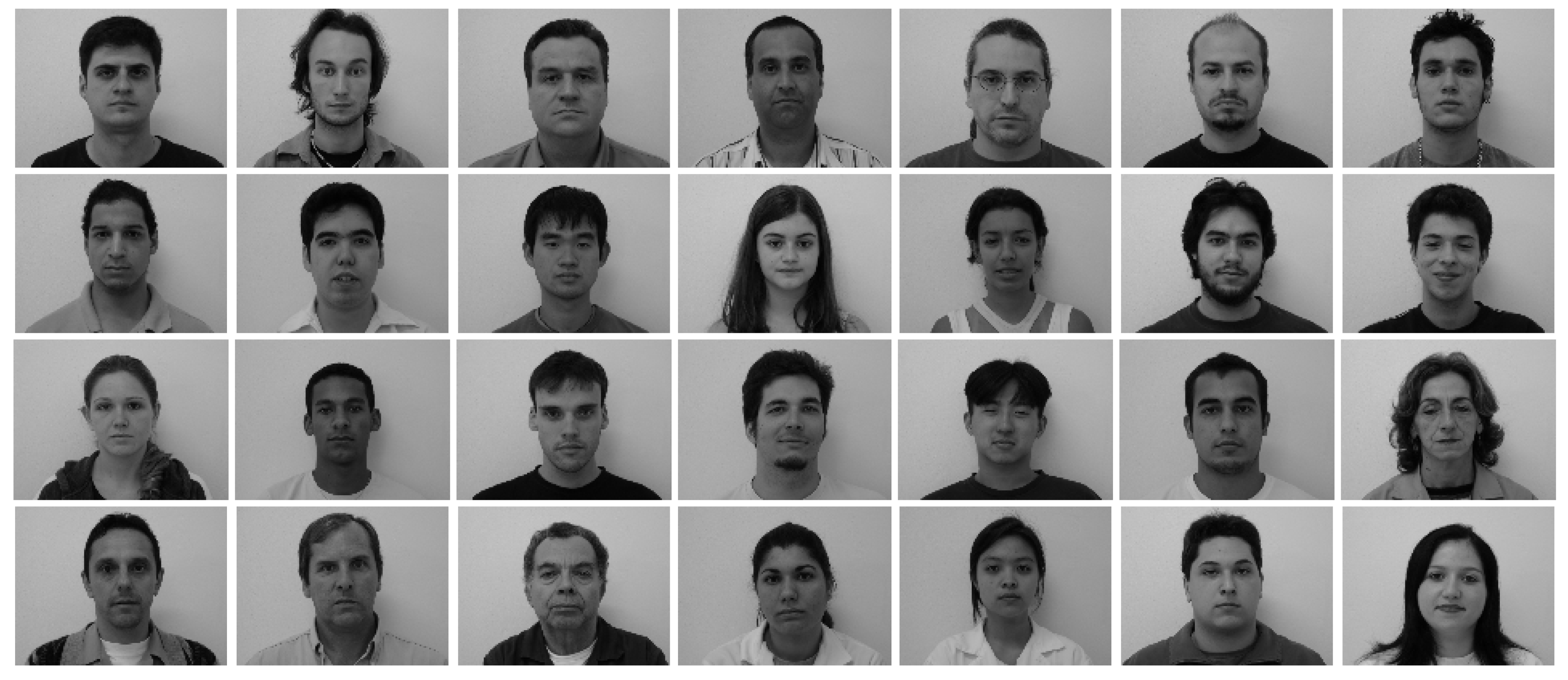
The second dataset is the FEI dataset [74] which is a Brazilian facial dataset. The FEI dataset is composed of 100 faces, including males and females. In the experiment we included ten images for each person, with a size of . The participants’ images have a neutral background, their age is between 19 and 40 years, and the dataset consists of faces with facial expressions and poses of various types. Figure 6 shows samples of the FEI face dataset.
The experiment wass performed for three different image sizes: the original size ( pixels), downsampled by a factor of two, and downsampled by a factor of four. Various block overlaps were tested. The accuracy is reported both for noise-free and noisy environments. The noise was Gaussian with two variance values and Salt and Pepper with two density values as depicted in Figure 7. The obtained results are reported in Table 5. The results show that the best overlap size for this dataset is one sixth of the block size. For example, with a block size of , the best overlap size is (8,8), for a block size of , the best overlap size is (4,4), and for a block size of , the best overlap size is (2,2). As these results were obtained from a large image database, it is highly probable that these conclusions are valid for other datasets of a similar kind.
In order to illustrate the efficiency of our fast block processing method, the proposed algorithm was compared to an algorithm that processes the blocks sequentially. The experiment was performed with an image size of , a block size of , and for different overlap sizes, as shown in Table 6, where the runtime in seconds is provided. The results show that the proposed algorithm outperforms the traditional one for all overlap sizes (obviously, larger overlap sizes lead to a higher improvement). The average incease in speed is about 50 times, which is quite impressive.
Finally, we compared the proposed algorithm to eleven state-of-the-art face recognition algorithms. The recognition rates are shown in Table 7. It can be observed that, at least on this database, the proposed algorithm outperforms all compared algorithms.
5. Conclusions
In this paper, we have proposed a new face recognition method. It belongs to the category of “handcrafted” features-based techniques. Unlike deep learning methods, it does not require any time-consuming massive training on augmented datasets. The method is a cascade of several steps. The image is partitioned into overlapping blocks, which makes the method robust to local changes. Each block is described by orthogonal moments with respect to a carefully chosen polynomial basis. A noise-suppression filter is embedded into moment calculation with almost no overheads. This makes the method particularly efficient in recognition of noisy faces. High computational efficiency is ensured by an original fast block processing method that avoids treatment of blocks in slow loops. All these ideas together, when implemented into a single framework, result in a fast, robust, and reliable face recognition method, as demonstrated in this paper by numerous experiments. To increase the recognition accuracy, future research could further examine noisy environments using a non-local mean filter as an alternative to the embedded Gaussian filter.
Author Contributions
Conceptualization, S.H.A. and B.M.M.; methodology, S.H.A. and B.M.M.; software, S.H.A. and B.M.M.; validation, J.F. and A.A.; investigation, A.A., and B.M.M.; resources, J.F. and S.H.A.; writing—original draft preparation, S.H.A., J.F., B.M.M. and A.A.; writing—review and editing, J.F. and A.A.; visualization, A.A. and B.M.M.; project administration, S.H.A. and J.F. All authors have read and agreed to the published version of the manuscript.
Funding
This research received no external funding.
Institutional Review Board Statement
Not applicable.
Informed Consent Statement
Not applicable.
Data Availability Statement
All the links and how to obtain the presented data in this paper, if publicly available, can be found through the referenced papers.
Acknowledgments
The authors would like to thank the University of Baghdad and University of Hai’l for their help and support. Jan Flusser has been supported by the Czech Science Foundation under the grant No. GA21-03921S, by the Praemium Academiae, and by Joint Laboratory Salome 2.
Conflicts of Interest
The authors declare no conflict of interest.
Abbreviations
The following abbreviations are used in this manuscript:
| 2D | Two-dimensional |
| FOBP | Fast Overlapped Block Processing |
| HOP | Hybrid Orthogonal Polynomials |
| KPs | Krawtchouk polynomials |
| OP | Orthogonal Polynomials |
| OM | Orthogonal Moments |
| PSNR | Peak Signal-to-Noise Ratio |
| SKTM | Squared Krawtchouk–Tchebichef Moment |
| SKTP | Squared Krawtchouk–Tchebichef polynomials |
| TPs | Tchebichef polynomials |
Appendix A. Computation of the KP and TP Coefficients
Appendix A.1. Computation of the KP Coefficients
This section introduces the utilized recurrence relation for the KP. Recurrence relations are commonly used for the sake of numerical stability and speed when evaluating orthogonal polynomials.
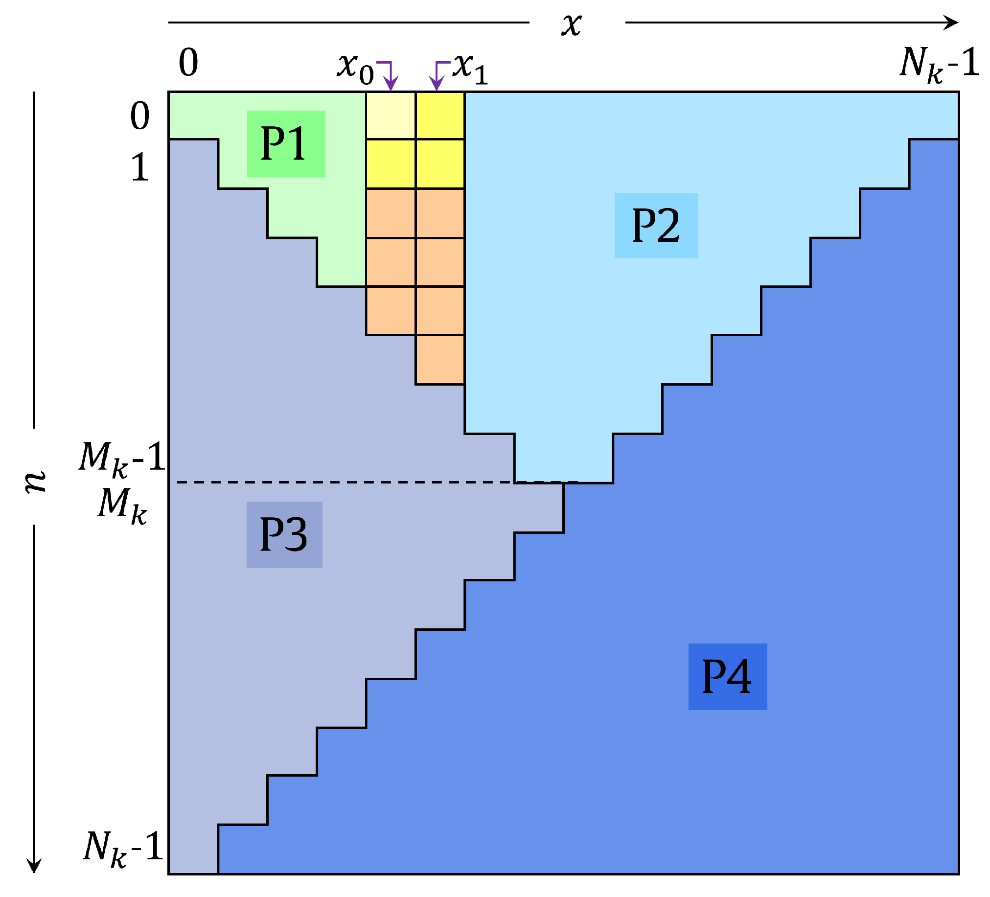
The procedure used to generate the KP of the n-th order and size is as follows (please refer to Figure A1 for the parts of the KP) [93]:
Figure A1.
Parts of the KP.

- 1.
- The initial values are computed as follows:
- 1.1.
- The value at and is computed bywhere . Note that represents the logarithmic Gamma function.
- 1.2.
- The value at and is computed by
- 1.3.
- The value at and are computed by
- 1.4.
- The values in the range and are computed by
- 2.
- The values in part P1 () are computed as follows:with the condition . This condition is used to prevent underflow in high orders of the Krawtchouk polynomials.
- 3.
- The values in part P2 are computed as follows:
- 3.1.
- the values in the range () are provided bywith the condition .
- 3.2.
- The values in the range () are provided by
- 3.3.
- The values in the range ( and ) are provided by Equation (25).
- 4.
- To compute the rest of the KP coefficients, the following relations are used:
- 4.1.
- The values in the range and are computed using
- 4.2.
- The values in the range and are computed using
The reason for using the algorithm presented in [93] is that it shows high stability in computation of the KP coefficients.
Appendix A.2. Computation of the TP Coefficients
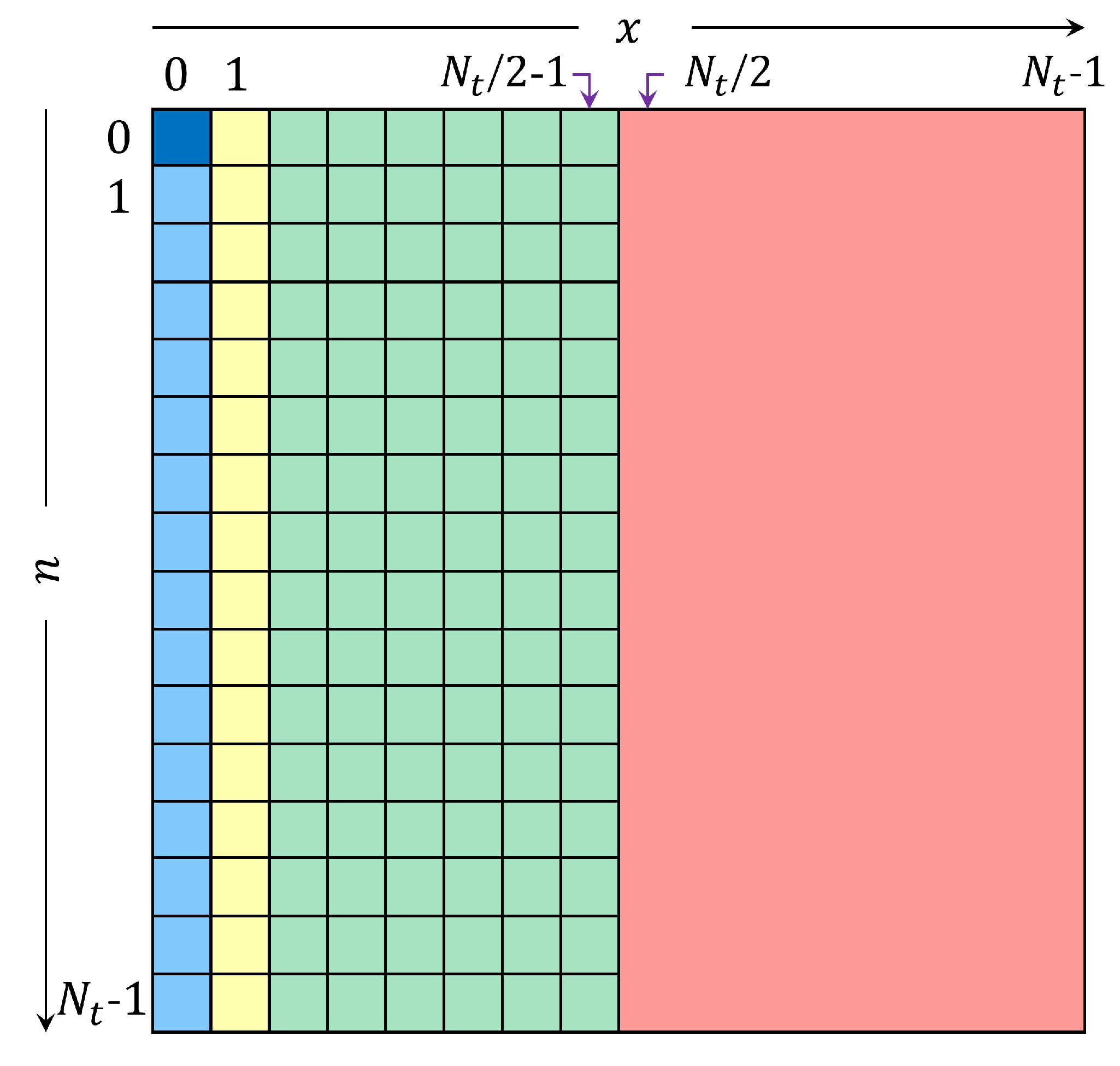
The algorithm presented in [94] is utilized to compute the coefficients of the TP. The procedure presented in [94] to compute the n-th order with a size of is as follows (please see Figure A2):
Figure A2.
Parts of the TP.

- 1.
- The initial set of values are computed as follows:
- 1.1.
- The initial value at is computed by
- 1.2.
- The initial values at the range and are computed by
- 1.3.
- The initial values at the range and are computed by
- 2.
- The values in the range are computed by
- 3.
- The values in the range and are computed using the relation
Appendix B. Detailed Results of the Individual Runs for Different σ Values for the Used Smoothing Kernel
This section presents the detailed results of the 20 runs for different environments using different values of for the utilized smoothing kernel.

Table A1.
The results of the runs for noise-free environment using different values of .
| Run ID | |||||||||
|---|---|---|---|---|---|---|---|---|---|
| Overlap Size | Overlap Size | Overlap Size | |||||||
| (0,0) | (2,2) | (4,4) | (0,0) | (2,2) | (4,4) | (0,0) | (2,2) | (4,4) | |
| 1 | 97.00 | 98.00 | 97.50 | 97.50 | 97.50 | 97.50 | 97.50 | 97.00 | 97.50 |
| 2 | 99.00 | 99.00 | 99.00 | 99.00 | 98.50 | 99.50 | 99.50 | 98.50 | 99.50 |
| 3 | 97.00 | 98.00 | 97.00 | 97.00 | 96.00 | 97.00 | 96.00 | 95.50 | 97.50 |
| 4 | 98.00 | 97.50 | 97.50 | 98.00 | 97.50 | 98.00 | 97.50 | 97.50 | 97.00 |
| 5 | 98.50 | 98.00 | 97.50 | 99.00 | 98.00 | 98.00 | 98.50 | 97.50 | 98.50 |
| 6 | 97.50 | 97.50 | 98.00 | 97.50 | 98.50 | 99.00 | 98.50 | 98.00 | 99.00 |
| 7 | 96.50 | 96.50 | 97.00 | 97.00 | 97.00 | 97.50 | 97.00 | 97.00 | 97.50 |
| 8 | 98.50 | 97.50 | 98.00 | 97.50 | 98.00 | 98.50 | 97.50 | 98.00 | 98.00 |
| 9 | 96.50 | 96.00 | 96.50 | 96.50 | 96.00 | 97.00 | 96.50 | 95.50 | 97.00 |
| 10 | 97.50 | 97.50 | 98.00 | 97.50 | 98.50 | 99.00 | 98.50 | 98.00 | 99.00 |
| 11 | 98.00 | 98.00 | 97.00 | 98.50 | 98.50 | 98.50 | 99.00 | 99.00 | 99.00 |
| 12 | 98.00 | 98.00 | 98.00 | 98.00 | 97.50 | 98.00 | 97.00 | 97.00 | 96.50 |
| 13 | 95.00 | 95.50 | 96.00 | 96.00 | 96.00 | 96.50 | 96.50 | 96.00 | 97.00 |
| 14 | 98.50 | 98.50 | 98.00 | 99.00 | 98.50 | 99.00 | 99.00 | 98.50 | 98.50 |
| 15 | 99.00 | 99.00 | 99.00 | 98.50 | 98.50 | 99.00 | 98.50 | 99.00 | 98.50 |
| 16 | 98.50 | 98.50 | 98.00 | 98.50 | 99.00 | 99.00 | 98.50 | 99.00 | 98.50 |
| 17 | 98.50 | 98.00 | 96.50 | 98.00 | 98.00 | 98.50 | 97.50 | 97.50 | 98.50 |
| 18 | 97.00 | 97.50 | 97.00 | 98.00 | 97.50 | 98.50 | 98.50 | 97.50 | 97.00 |
| 19 | 97.50 | 97.50 | 98.50 | 97.50 | 98.00 | 98.50 | 97.50 | 98.00 | 98.00 |
| 20 | 98.50 | 97.50 | 99.00 | 96.50 | 97.50 | 98.00 | 96.50 | 97.50 | 97.50 |
| Average | 97.73 | 97.68 | 97.65 | 97.75 | 97.73 | 98.23 | 97.78 | 97.58 | 97.98 |
Table A2.
The results of the runs for Gaussian noise with standard deviation of 0.01 using different values of .
Table A2.
The results of the runs for Gaussian noise with standard deviation of 0.01 using different values of .
| Run ID | |||||||||
|---|---|---|---|---|---|---|---|---|---|
| Overlap Size | Overlap Size | Overlap Size | |||||||
| (0,0) | (2,2) | (4,4) | (0,0) | (2,2) | (4,4) | (0,0) | (2,2) | (4,4) | |
| 1 | 97.00 | 97.50 | 97.50 | 97.50 | 97.50 | 97.50 | 97.50 | 97.50 | 97.50 |
| 2 | 99.00 | 99.00 | 99.00 | 99.00 | 98.50 | 99.50 | 99.50 | 98.50 | 99.50 |
| 3 | 97.00 | 97.50 | 96.50 | 97.00 | 96.00 | 97.00 | 96.00 | 96.00 | 97.50 |
| 4 | 98.50 | 98.00 | 97.50 | 98.00 | 98.00 | 98.00 | 97.50 | 97.50 | 97.00 |
| 5 | 98.50 | 98.50 | 98.00 | 99.00 | 98.50 | 98.00 | 98.50 | 98.00 | 98.50 |
| 6 | 97.00 | 97.50 | 98.00 | 97.50 | 99.00 | 99.00 | 98.50 | 98.00 | 99.00 |
| 7 | 96.50 | 96.50 | 96.50 | 97.00 | 97.00 | 97.50 | 97.00 | 97.00 | 97.50 |
| 8 | 98.00 | 97.50 | 98.00 | 98.00 | 98.00 | 98.50 | 97.50 | 99.00 | 98.00 |
| 9 | 97.00 | 96.50 | 96.50 | 96.50 | 96.00 | 97.00 | 96.50 | 96.00 | 97.00 |
| 10 | 97.00 | 97.50 | 98.00 | 97.50 | 99.00 | 99.00 | 98.50 | 98.00 | 99.00 |
| 11 | 98.00 | 98.00 | 97.50 | 98.50 | 98.50 | 98.50 | 99.00 | 99.00 | 99.00 |
| 12 | 98.50 | 97.50 | 97.50 | 97.50 | 98.00 | 98.50 | 97.00 | 96.50 | 96.50 |
| 13 | 94.50 | 95.50 | 95.50 | 95.50 | 96.00 | 96.50 | 96.50 | 96.00 | 96.50 |
| 14 | 98.50 | 98.50 | 98.00 | 99.00 | 98.50 | 99.00 | 98.50 | 98.50 | 98.50 |
| 15 | 99.50 | 99.00 | 99.00 | 98.00 | 99.00 | 99.00 | 98.50 | 99.00 | 98.50 |
| 16 | 98.50 | 98.50 | 98.00 | 98.50 | 99.00 | 99.00 | 98.50 | 99.00 | 98.50 |
| 17 | 98.00 | 98.00 | 96.50 | 98.00 | 98.00 | 98.50 | 97.50 | 97.50 | 98.50 |
| 18 | 97.50 | 97.50 | 96.50 | 97.00 | 97.50 | 98.00 | 98.50 | 97.50 | 97.00 |
| 19 | 97.50 | 98.00 | 98.50 | 97.50 | 97.50 | 98.50 | 97.50 | 98.00 | 98.50 |
| 20 | 98.50 | 97.50 | 98.50 | 96.50 | 97.50 | 98.00 | 97.00 | 97.50 | 97.50 |
| Average | 97.73 | 97.70 | 97.55 | 97.65 | 97.85 | 98.23 | 97.78 | 97.70 | 97.98 |
Table A3.
The results of the runs for Gaussian noise with standard deviation of 0.05 using different values of .
Table A3.
The results of the runs for Gaussian noise with standard deviation of 0.05 using different values of .
| Run ID | |||||||||
|---|---|---|---|---|---|---|---|---|---|
| Overlap Size | Overlap Size | Overlap Size | |||||||
| (0,0) | (2,2) | (4,4) | (0,0) | (2,2) | (4,4) | (0,0) | (2,2) | (4,4) | |
| 1 | 97.00 | 97.50 | 98.00 | 97.50 | 97.50 | 97.50 | 97.50 | 97.50 | 97.50 |
| 2 | 99.00 | 99.00 | 98.50 | 99.00 | 98.50 | 99.50 | 99.50 | 98.00 | 99.50 |
| 3 | 97.00 | 98.00 | 97.00 | 96.00 | 96.00 | 97.00 | 96.00 | 96.00 | 97.00 |
| 4 | 98.50 | 97.50 | 98.00 | 98.00 | 98.00 | 97.00 | 96.50 | 97.50 | 97.00 |
| 5 | 98.50 | 98.00 | 97.50 | 99.00 | 98.50 | 98.50 | 98.50 | 98.00 | 99.00 |
| 6 | 97.50 | 97.50 | 98.00 | 97.50 | 98.50 | 99.00 | 98.00 | 98.00 | 99.00 |
| 7 | 96.50 | 96.50 | 97.00 | 97.00 | 97.00 | 97.50 | 97.00 | 97.00 | 97.50 |
| 8 | 97.50 | 98.00 | 98.50 | 97.50 | 98.00 | 98.50 | 97.50 | 98.00 | 98.00 |
| 9 | 96.50 | 96.00 | 96.00 | 96.00 | 96.00 | 97.00 | 96.50 | 95.50 | 97.50 |
| 10 | 97.50 | 97.50 | 98.00 | 97.50 | 98.50 | 99.00 | 98.00 | 98.00 | 99.00 |
| 11 | 98.00 | 97.50 | 97.00 | 98.50 | 98.50 | 98.50 | 99.00 | 99.50 | 98.50 |
| 12 | 98.50 | 98.50 | 98.00 | 97.50 | 98.00 | 98.00 | 96.50 | 97.00 | 96.50 |
| 13 | 95.50 | 95.50 | 95.50 | 96.00 | 96.00 | 97.00 | 96.00 | 96.00 | 97.00 |
| 14 | 98.50 | 98.50 | 98.50 | 99.00 | 98.50 | 99.00 | 99.00 | 98.50 | 98.50 |
| 15 | 99.00 | 98.50 | 99.00 | 98.00 | 98.50 | 99.00 | 98.50 | 99.00 | 98.50 |
| 16 | 98.50 | 98.50 | 98.00 | 98.50 | 99.00 | 99.00 | 98.50 | 99.00 | 99.00 |
| 17 | 98.00 | 98.00 | 97.50 | 98.00 | 98.00 | 98.50 | 97.50 | 97.50 | 98.50 |
| 18 | 97.00 | 97.50 | 97.00 | 98.00 | 97.50 | 98.50 | 98.50 | 97.00 | 97.00 |
| 19 | 97.50 | 98.00 | 98.50 | 97.50 | 98.00 | 98.00 | 97.50 | 98.00 | 98.00 |
| 20 | 98.00 | 96.50 | 98.00 | 96.00 | 97.50 | 97.50 | 96.00 | 97.00 | 97.50 |
| Average | 97.70 | 97.63 | 97.68 | 97.60 | 97.80 | 98.18 | 97.60 | 97.60 | 98.00 |
Table A4.
The results of the runs for Salt and Pepper noise with density of 0.05 using different values of .
Table A4.
The results of the runs for Salt and Pepper noise with density of 0.05 using different values of .
| Run ID | |||||||||
|---|---|---|---|---|---|---|---|---|---|
| Overlap Size | Overlap Size | Overlap Size | |||||||
| (0,0) | (2,2) | (4,4) | (0,0) | (2,2) | (4,4) | (0,0) | (2,2) | (4,4) | |
| 1 | 97.50 | 97.50 | 98.50 | 97.50 | 98.00 | 97.50 | 97.50 | 98.00 | 97.50 |
| 2 | 99.50 | 98.50 | 99.50 | 99.00 | 99.00 | 99.50 | 99.00 | 99.00 | 99.50 |
| 3 | 96.50 | 97.50 | 97.50 | 96.50 | 97.00 | 97.00 | 96.00 | 96.00 | 97.00 |
| 4 | 97.50 | 97.00 | 97.00 | 97.50 | 96.50 | 96.50 | 97.00 | 96.50 | 96.50 |
| 5 | 98.50 | 98.50 | 98.00 | 99.00 | 98.50 | 99.00 | 98.50 | 98.50 | 99.00 |
| 6 | 97.50 | 97.50 | 97.50 | 97.50 | 99.00 | 98.50 | 98.00 | 98.50 | 98.50 |
| 7 | 97.00 | 96.00 | 97.00 | 97.00 | 97.00 | 97.50 | 97.00 | 97.00 | 97.50 |
| 8 | 98.50 | 97.50 | 98.50 | 97.50 | 98.00 | 98.50 | 97.50 | 98.50 | 98.00 |
| 9 | 96.50 | 96.00 | 96.00 | 96.00 | 96.50 | 96.50 | 96.00 | 96.00 | 96.50 |
| 10 | 97.50 | 97.50 | 97.50 | 97.50 | 99.00 | 98.50 | 98.00 | 98.50 | 98.50 |
| 11 | 97.50 | 98.00 | 97.50 | 98.00 | 98.50 | 98.50 | 99.00 | 99.50 | 98.50 |
| 12 | 98.00 | 97.00 | 97.00 | 97.00 | 96.50 | 97.00 | 96.50 | 96.00 | 95.50 |
| 13 | 96.00 | 95.00 | 96.50 | 95.50 | 97.00 | 96.50 | 96.50 | 96.50 | 97.00 |
| 14 | 99.00 | 98.50 | 98.50 | 99.00 | 98.50 | 99.00 | 98.50 | 98.50 | 98.50 |
| 15 | 98.00 | 98.50 | 98.50 | 98.00 | 98.50 | 98.50 | 98.50 | 98.50 | 98.50 |
| 16 | 98.50 | 98.50 | 98.00 | 98.50 | 99.00 | 99.00 | 98.50 | 98.50 | 99.00 |
| 17 | 97.50 | 98.00 | 97.50 | 97.50 | 98.50 | 98.00 | 97.50 | 97.50 | 98.00 |
| 18 | 97.50 | 97.50 | 97.50 | 97.50 | 98.00 | 98.50 | 98.50 | 98.00 | 97.50 |
| 19 | 97.50 | 97.50 | 98.50 | 98.00 | 97.00 | 98.00 | 98.00 | 97.50 | 98.00 |
| 20 | 96.50 | 96.00 | 97.50 | 96.00 | 97.00 | 97.00 | 96.50 | 97.00 | 96.50 |
| Average | 97.63 | 97.40 | 97.70 | 97.50 | 97.85 | 97.95 | 97.63 | 97.70 | 97.78 |
Table A5.
The results of the runs for Salt and Pepper noise with density of 0.10 using different values of .
Table A5.
The results of the runs for Salt and Pepper noise with density of 0.10 using different values of .
| Run ID | |||||||||
|---|---|---|---|---|---|---|---|---|---|
| Overlap Size | Overlap Size | Overlap Size | |||||||
| (0,0) | (2,2) | (4,4) | (0,0) | (2,2) | (4,4) | (0,0) | (2,2) | (4,4) | |
| 1 | 98.00 | 97.50 | 98.00 | 97.50 | 97.00 | 98.00 | 98.00 | 97.00 | 97.00 |
| 2 | 98.00 | 98.50 | 97.50 | 98.00 | 98.50 | 99.50 | 99.00 | 98.50 | 99.50 |
| 3 | 98.00 | 97.50 | 97.50 | 96.00 | 97.00 | 96.50 | 96.00 | 95.00 | 96.50 |
| 4 | 97.50 | 95.00 | 97.00 | 96.50 | 96.50 | 96.00 | 96.50 | 96.00 | 96.50 |
| 5 | 98.50 | 97.50 | 97.50 | 98.50 | 97.50 | 98.50 | 98.00 | 98.00 | 98.00 |
| 6 | 97.50 | 98.00 | 97.50 | 97.50 | 97.50 | 98.50 | 97.00 | 97.50 | 98.50 |
| 7 | 97.00 | 96.00 | 97.00 | 97.00 | 97.00 | 97.50 | 97.00 | 97.00 | 97.50 |
| 8 | 99.00 | 97.50 | 98.50 | 97.50 | 97.00 | 98.50 | 97.50 | 98.00 | 98.50 |
| 9 | 96.50 | 95.00 | 96.00 | 95.50 | 95.50 | 96.00 | 95.50 | 95.00 | 95.50 |
| 10 | 97.50 | 98.00 | 97.50 | 97.50 | 97.50 | 98.50 | 97.00 | 97.50 | 98.50 |
| 11 | 97.00 | 96.50 | 96.50 | 97.00 | 98.00 | 98.00 | 97.00 | 98.00 | 97.50 |
| 12 | 96.50 | 95.50 | 96.00 | 95.00 | 94.50 | 95.50 | 95.50 | 94.50 | 94.00 |
| 13 | 95.00 | 95.00 | 94.50 | 95.00 | 94.00 | 95.00 | 94.50 | 94.50 | 94.50 |
| 14 | 99.00 | 98.50 | 98.50 | 98.50 | 98.50 | 98.50 | 98.50 | 98.50 | 98.50 |
| 15 | 98.50 | 98.50 | 98.50 | 98.00 | 98.50 | 98.50 | 98.50 | 98.50 | 98.00 |
| 16 | 98.50 | 98.00 | 98.00 | 98.50 | 98.00 | 98.50 | 98.50 | 98.00 | 98.00 |
| 17 | 98.00 | 98.50 | 98.00 | 97.00 | 98.00 | 98.00 | 97.50 | 97.50 | 98.00 |
| 18 | 97.50 | 97.50 | 97.00 | 97.00 | 97.00 | 98.00 | 97.50 | 97.00 | 96.50 |
| 19 | 97.50 | 96.50 | 98.50 | 97.50 | 96.50 | 97.50 | 98.00 | 96.50 | 98.00 |
| 20 | 95.50 | 95.00 | 97.50 | 96.00 | 95.50 | 96.50 | 96.50 | 95.50 | 96.50 |
| Average | 97.53 | 97.00 | 97.35 | 97.05 | 96.98 | 97.58 | 97.18 | 96.90 | 97.28 |
Appendix C. The Detailed Results of the Individual Runs with and without Smoothing Kernel
In this section, the detailed results of the 20 runs for different environments with and without a smoothing kernel are shown.
Table A6.
The results of the runs for noise-free environment.
| Run ID | Without Smoothing Kernel | With Smoothing Kernel | ||||
|---|---|---|---|---|---|---|
| Overlap Size | Overlap Size | |||||
| (0,0) | (2,2) | (4,4) | (0,0) | (2,2) | (4,4) | |
| 1 | 97.50 | 98.00 | 97.00 | 97.50 | 97.50 | 97.50 |
| 2 | 98.50 | 99.00 | 99.00 | 99.00 | 98.50 | 99.50 |
| 3 | 96.00 | 98.00 | 97.50 | 97.00 | 96.00 | 97.00 |
| 4 | 97.50 | 97.00 | 98.50 | 98.00 | 97.50 | 98.00 |
| 5 | 97.50 | 98.50 | 98.50 | 99.00 | 98.00 | 98.00 |
| 6 | 97.50 | 97.00 | 97.50 | 97.50 | 98.50 | 99.00 |
| 7 | 97.00 | 96.50 | 96.50 | 97.00 | 97.00 | 97.50 |
| 8 | 98.00 | 97.00 | 97.50 | 97.50 | 98.00 | 98.50 |
| 9 | 96.00 | 96.50 | 97.00 | 96.50 | 96.00 | 97.00 |
| 10 | 97.50 | 97.00 | 97.50 | 97.50 | 98.50 | 99.00 |
| 11 | 97.00 | 97.00 | 98.00 | 98.50 | 98.50 | 98.50 |
| 12 | 97.00 | 97.50 | 97.50 | 98.00 | 97.50 | 98.00 |
| 13 | 95.00 | 95.00 | 94.50 | 96.00 | 96.00 | 96.50 |
| 14 | 98.00 | 98.50 | 98.50 | 99.00 | 98.50 | 99.00 |
| 15 | 99.00 | 99.00 | 99.50 | 98.50 | 98.50 | 99.00 |
| 16 | 98.00 | 98.50 | 98.50 | 98.50 | 99.00 | 99.00 |
| 17 | 96.50 | 98.00 | 97.00 | 98.00 | 98.00 | 98.50 |
| 18 | 97.00 | 97.50 | 97.00 | 98.00 | 97.50 | 98.50 |
| 19 | 98.50 | 97.00 | 97.50 | 97.50 | 98.00 | 98.50 |
| 20 | 98.00 | 97.50 | 97.50 | 96.50 | 97.50 | 98.00 |
| Average | 97.35 | 97.50 | 97.60 | 97.75 | 97.73 | 98.23 |
Table A7.
The results of the runs for Gaussian noise with standard deviation of 0.01.
| Run ID | Without Smoothing Kernel | With Smoothing Kernel | ||||
|---|---|---|---|---|---|---|
| Overlap Size | Overlap Size | |||||
| (0,0) | (2,2) | (4,4) | (0,0) | (2,2) | (4,4) | |
| 1 | 97.00 | 97.50 | 97.00 | 97.50 | 97.50 | 97.50 |
| 2 | 98.50 | 99.00 | 98.50 | 99.00 | 98.50 | 99.50 |
| 3 | 96.50 | 98.00 | 97.50 | 97.00 | 96.00 | 97.00 |
| 4 | 97.50 | 97.50 | 98.00 | 98.00 | 98.00 | 98.00 |
| 5 | 97.50 | 98.50 | 98.50 | 99.00 | 98.50 | 98.00 |
| 6 | 97.50 | 97.00 | 97.00 | 97.50 | 99.00 | 99.00 |
| 7 | 96.50 | 96.50 | 96.50 | 97.00 | 97.00 | 97.50 |
| 8 | 98.00 | 97.00 | 98.50 | 98.00 | 98.00 | 98.50 |
| 9 | 96.00 | 96.50 | 96.50 | 96.50 | 96.00 | 97.00 |
| 10 | 97.50 | 97.00 | 97.00 | 97.50 | 99.00 | 99.00 |
| 11 | 97.00 | 97.00 | 98.00 | 98.50 | 98.50 | 98.50 |
| 12 | 96.50 | 97.00 | 97.50 | 97.50 | 98.00 | 98.50 |
| 13 | 95.00 | 95.00 | 94.50 | 95.50 | 96.00 | 96.50 |
| 14 | 98.00 | 98.50 | 98.50 | 99.00 | 98.50 | 99.00 |
| 15 | 99.00 | 99.00 | 99.50 | 98.00 | 99.00 | 99.00 |
| 16 | 98.00 | 98.50 | 98.50 | 98.50 | 99.00 | 99.00 |
| 17 | 96.50 | 98.00 | 97.50 | 98.00 | 98.00 | 98.50 |
| 18 | 97.00 | 97.50 | 98.00 | 97.00 | 97.50 | 98.00 |
| 19 | 98.50 | 97.50 | 97.50 | 97.50 | 97.50 | 98.50 |
| 20 | 98.50 | 98.00 | 97.50 | 96.50 | 97.50 | 98.00 |
| Average | 97.33 | 97.53 | 97.60 | 97.65 | 97.85 | 98.23 |
Table A8.
The results of the runs for Gaussian noise with standard deviation of 0.05.
| Run ID | Without Smoothing Kernel | With Smoothing Kernel | ||||
|---|---|---|---|---|---|---|
| Overlap Size | Overlap Size | |||||
| (0,0) | (2,2) | (4,4) | (0,0) | (2,2) | (4,4) | |
| 1 | 98.00 | 98.00 | 97.00 | 97.50 | 97.50 | 97.50 |
| 2 | 98.00 | 99.00 | 98.50 | 99.00 | 98.50 | 99.50 |
| 3 | 97.00 | 98.00 | 97.50 | 96.00 | 96.00 | 97.00 |
| 4 | 97.50 | 96.50 | 98.50 | 98.00 | 98.00 | 97.00 |
| 5 | 97.50 | 98.50 | 98.00 | 99.00 | 98.50 | 98.50 |
| 6 | 98.00 | 97.50 | 97.50 | 97.50 | 98.50 | 99.00 |
| 7 | 97.00 | 96.50 | 96.50 | 97.00 | 97.00 | 97.50 |
| 8 | 98.00 | 98.00 | 97.50 | 97.50 | 98.00 | 98.50 |
| 9 | 96.00 | 96.00 | 96.00 | 96.00 | 96.00 | 97.00 |
| 10 | 98.00 | 97.50 | 97.50 | 97.50 | 98.50 | 99.00 |
| 11 | 96.00 | 97.00 | 97.50 | 98.50 | 98.50 | 98.50 |
| 12 | 98.00 | 98.50 | 98.00 | 97.50 | 98.00 | 98.00 |
| 13 | 95.50 | 95.00 | 95.00 | 96.00 | 96.00 | 97.00 |
| 14 | 98.00 | 98.50 | 98.50 | 99.00 | 98.50 | 99.00 |
| 15 | 98.50 | 99.00 | 99.00 | 98.00 | 98.50 | 99.00 |
| 16 | 98.00 | 98.50 | 98.50 | 98.50 | 99.00 | 99.00 |
| 17 | 97.00 | 98.00 | 98.00 | 98.00 | 98.00 | 98.50 |
| 18 | 96.50 | 97.50 | 97.00 | 98.00 | 97.50 | 98.50 |
| 19 | 98.50 | 97.50 | 97.50 | 97.50 | 98.00 | 98.00 |
| 20 | 97.00 | 96.50 | 97.50 | 96.00 | 97.50 | 97.50 |
| Average | 97.40 | 97.58 | 97.55 | 97.60 | 97.80 | 98.18 |
Table A9.
The results of the runs for Salt and Pepper noise with density of 0.05.
| Run ID | Without Smoothing Kernel | With Smoothing Kernel | ||||
|---|---|---|---|---|---|---|
| Overlap Size | Overlap Size | |||||
| (0,0) | (2,2) | (4,4) | (0,0) | (2,2) | (4,4) | |
| 1 | 98.00 | 98.50 | 97.50 | 97.50 | 98.00 | 97.50 |
| 2 | 98.50 | 99.00 | 99.00 | 99.00 | 99.00 | 99.50 |
| 3 | 97.50 | 99.00 | 96.50 | 96.50 | 97.00 | 97.00 |
| 4 | 96.50 | 97.00 | 97.50 | 97.50 | 96.50 | 96.50 |
| 5 | 97.50 | 98.50 | 98.00 | 99.00 | 98.50 | 99.00 |
| 6 | 97.50 | 97.50 | 97.50 | 97.50 | 99.00 | 98.50 |
| 7 | 97.00 | 96.00 | 97.00 | 97.00 | 97.00 | 97.50 |
| 8 | 98.00 | 97.50 | 98.50 | 97.50 | 98.00 | 98.50 |
| 9 | 96.00 | 96.50 | 97.00 | 96.00 | 96.50 | 96.50 |
| 10 | 97.50 | 97.50 | 97.50 | 97.50 | 99.00 | 98.50 |
| 11 | 97.00 | 97.50 | 97.50 | 98.00 | 98.50 | 98.50 |
| 12 | 97.00 | 97.00 | 98.00 | 97.00 | 96.50 | 97.00 |
| 13 | 97.00 | 95.50 | 96.00 | 95.50 | 97.00 | 96.50 |
| 14 | 98.50 | 98.50 | 99.00 | 99.00 | 98.50 | 99.00 |
| 15 | 99.00 | 98.50 | 98.00 | 98.00 | 98.50 | 98.50 |
| 16 | 98.00 | 98.50 | 98.00 | 98.50 | 99.00 | 99.00 |
| 17 | 97.50 | 98.00 | 97.50 | 97.50 | 98.50 | 98.00 |
| 18 | 97.50 | 97.50 | 97.50 | 97.50 | 98.00 | 98.50 |
| 19 | 98.50 | 97.00 | 97.50 | 98.00 | 97.00 | 98.00 |
| 20 | 98.00 | 97.00 | 96.50 | 96.00 | 97.00 | 97.00 |
| Average | 97.60 | 97.60 | 97.58 | 97.50 | 97.85 | 97.95 |
Table A10.
The results of the runs for Salt and Pepper noise with density of 0.10.
| Run ID | Without Smoothing Kernel | With Smoothing Kernel | ||||
|---|---|---|---|---|---|---|
| Overlap Size | Overlap Size | |||||
| (0,0) | (2,2) | (4,4) | (0,0) | (2,2) | (4,4) | |
| 1 | 97.00 | 98.00 | 97.50 | 97.50 | 97.00 | 98.00 |
| 2 | 98.00 | 98.50 | 98.00 | 98.00 | 98.50 | 99.50 |
| 3 | 97.00 | 98.50 | 95.50 | 96.00 | 97.00 | 96.50 |
| 4 | 96.00 | 96.00 | 97.00 | 96.50 | 96.50 | 96.00 |
| 5 | 97.50 | 98.50 | 98.00 | 98.50 | 97.50 | 98.50 |
| 6 | 97.50 | 98.00 | 97.50 | 97.50 | 97.50 | 98.50 |
| 7 | 96.50 | 96.00 | 97.00 | 97.00 | 97.00 | 97.50 |
| 8 | 98.50 | 97.50 | 99.00 | 97.50 | 97.00 | 98.50 |
| 9 | 96.00 | 95.00 | 96.50 | 95.50 | 95.50 | 96.00 |
| 10 | 97.50 | 98.00 | 97.50 | 97.50 | 97.50 | 98.50 |
| 11 | 96.00 | 96.50 | 97.00 | 97.00 | 98.00 | 98.00 |
| 12 | 96.00 | 95.50 | 96.50 | 95.00 | 94.50 | 95.50 |
| 13 | 94.50 | 94.50 | 95.50 | 95.00 | 94.00 | 95.00 |
| 14 | 98.50 | 98.00 | 99.00 | 98.50 | 98.50 | 98.50 |
| 15 | 97.50 | 98.50 | 98.50 | 98.00 | 98.50 | 98.50 |
| 16 | 98.00 | 98.00 | 98.00 | 98.50 | 98.00 | 98.50 |
| 17 | 98.00 | 98.50 | 97.00 | 97.00 | 98.00 | 98.00 |
| 18 | 96.50 | 97.00 | 96.50 | 97.00 | 97.00 | 98.00 |
| 19 | 98.00 | 96.50 | 97.50 | 97.50 | 96.50 | 97.50 |
| 20 | 97.00 | 95.00 | 95.50 | 96.00 | 95.50 | 96.50 |
| Average | 97.08 | 97.10 | 97.23 | 97.05 | 96.98 | 97.58 |
References
- Zhao, G.; Pietikainen, M. Dynamic texture recognition using local binary patterns with an application to facial expressions. IEEE Trans. Pattern Anal. Mach. Intell. 2007, 29, 915–928. [Google Scholar] [CrossRef] [PubMed] [Green Version]
- Hosny, K.M.; Abd Elaziz, M.; Darwish, M.M. Color face recognition using novel fractional-order multi-channel exponent moments. Neural Comput. Appl. 2021, 33, 5419–5435. [Google Scholar] [CrossRef]
- Kumar, V.V.; Murty, G.S.; Kumar, P.S. Classification of facial expressions based on transitions derived from third order neighborhood LBP. Glob. J. Comput. Sci. Technol. 2014, 14. [Google Scholar]
- Akheel, T.S.; Shree, V.U.; Mastani, S.A. Stochastic gradient descent linear collaborative discriminant regression classification based face recognition. Evol. Intell. 2022, 15, 1729–1743. [Google Scholar] [CrossRef]
- Zhang, Y.; Hu, C.; Lu, X. IL-GAN: Illumination-invariant representation learning for single sample face recognition. J. Vis. Commun. Image Represent. 2019, 59, 501–513. [Google Scholar] [CrossRef]
- Maafiri, A.; Elharrouss, O.; Rfifi, S.; Al-Maadeed, S.A.; Chougdali, K. DeepWTPCA-L1: A new deep face recognition model based on WTPCA-L1 norm features. IEEE Access 2021, 9, 65091–65100. [Google Scholar] [CrossRef]
- Ahmed, S.; Frikha, M.; Hussein, T.D.H.; Rahebi, J. Optimum feature selection with particle swarm optimization to face recognition system using Gabor wavelet transform and deep learning. BioMed Res. Int. 2021, 2021, 6621540. [Google Scholar] [CrossRef]
- Zhao, C.; Li, X.; Dong, Y. Learning blur invariant binary descriptor for face recognition. Neurocomputing 2020, 404, 34–40. [Google Scholar] [CrossRef]
- Chen, Z.; Wu, X.J.; Yin, H.F.; Kittler, J. Noise-robust dictionary learning with slack block-diagonal structure for face recognition. Pattern Recognit. 2020, 100, 107118. [Google Scholar] [CrossRef]
- Jain, A.K.; Li, S.Z. Handbook of Face Recognition; Springer: London, UK, 2011; Volume 1. [Google Scholar]
- Abdulhussain, S.H.; Ramli, A.R.; Mahmmod, B.M.; Saripan, M.I.; Al-Haddad, S.A.R.; Jassim, W.A. A New Hybrid form of Krawtchouk and Tchebichef Polynomials: Design and Application. J. Math. Imaging Vis. 2019, 61, 555–570. [Google Scholar] [CrossRef]
- Abdulhussain, S.H.; Mahmmod, B.M.; Flusser, J.; AL-Utaibi, K.A.; Sait, S.M. Fast Overlapping Block Processing Algorithm for Feature Extraction. Symmetry 2022, 14, 715. [Google Scholar] [CrossRef]
- Mehdipour Ghazi, M.; Kemal Ekenel, H. A comprehensive analysis of deep learning based representation for face recognition. In Proceedings of the IEEE Conference on Computer Vision and Pattern Recognition Workshops, Las Vegas, NV, USA, 26 June–1 July 2016; pp. 34–41. [Google Scholar]
- Guo, S.; Chen, S.; Li, Y. Face recognition based on convolutional neural network and support vector machine. In Proceedings of the 2016 IEEE International Conference on Information and Automation (ICIA), Ningbo, China, 1–3 August 2016; pp. 1787–1792. [Google Scholar]
- Han, C.; Shan, S.; Kan, M.; Wu, S.; Chen, X. Face recognition with contrastive convolution. In Proceedings of the European Conference on Computer Vision (ECCV), Munich, Germany, 8–14 September 2018; pp. 118–134. [Google Scholar]
- Schroff, F.; Kalenichenko, D.; Philbin, J. Facenet: A unified embedding for face recognition and clustering. In Proceedings of the IEEE Conference on Computer Vision and Pattern Recognition, Boston, MA, USA, 7–12 June 2015; pp. 815–823. [Google Scholar]
- Asad, M.; Hussain, A.; Mir, U. Low complexity hybrid holistic–landmark based approach for face recognition. Multimed. Tools Appl. 2021, 80, 30199–30212. [Google Scholar] [CrossRef]
- Hmimid, A.; Sayyouri, M.; Qjidaa, H. Fast computation of separable two-dimensional discrete invariant moments for image classification. Pattern Recognit. 2015, 48, 509–521. [Google Scholar] [CrossRef]
- Jassim, W.A.; Raveendran, P.; Mukundan, R. New orthogonal polynomials for speech signal and image processing. IET Signal Process. 2012, 6, 713–723. [Google Scholar] [CrossRef]
- Flusser, J.; Zitova, B.; Suk, T. Moments and Moment Invariants in Pattern Recognition; John Wiley & Sons: Chichester, UK, 2009. [Google Scholar]
- Rahman, S.M.; Howlader, T.; Hatzinakos, D. On the selection of 2D Krawtchouk moments for face recognition. Pattern Recognit. 2016, 54, 83–93. [Google Scholar] [CrossRef]
- Teh, C.H.; Chin, R.T. On image analysis by the methods of moments. IEEE Trans. Pattern Anal. Mach. Intell. 1988, 10, 496–513. [Google Scholar] [CrossRef]
- Chen, B.; Yu, M.; Su, Q.; Shim, H.J.; Shi, Y.Q. Fractional Quaternion Zernike Moments for Robust Color Image Copy-Move Forgery Detection. IEEE Access 2018, 6, 56637–56646. [Google Scholar] [CrossRef]
- Kaur, P.; Pannu, H.S.; Malhi, A.K. Plant disease recognition using fractional-order Zernike moments and SVM classifier. Neural Comput. Appl. 2019, 31, 8749–8768. [Google Scholar] [CrossRef]
- Bahaoui, Z.; Zenkouar, K.; Fadili, H.E.; Qjidaa, H.; Zarghili, A. Blocking artifact removal using partial overlapping based on exact Legendre moments computation. J. Real-Time Image Process. 2018, 14, 433–451. [Google Scholar] [CrossRef]
- Teague, M.R. Image analysis via the general theory of moments. Josa 1980, 70, 920–930. [Google Scholar] [CrossRef]
- Mahmmod, B.M.; bin Ramli, A.R.; Abdulhussain, S.H.; Al-Haddad, S.A.R.; Jassim, W.A. Signal compression and enhancement using a new orthogonal-polynomial-based discrete transform. IET Signal Process. 2018, 12, 129–142. [Google Scholar] [CrossRef]
- Yang, B.; Dai, M. Image analysis by Gaussian–Hermite moments. Signal Process. 2011, 91, 2290–2303. [Google Scholar] [CrossRef]
- Mukundan, R.; Ong, S.; Lee, P.A. Image analysis by Tchebichef moments. IEEE Trans. Image Process. 2001, 10, 1357–1364. [Google Scholar] [CrossRef] [PubMed]
- Xiao, B.; Luo, J.; Bi, X.; Li, W.; Chen, B. Fractional discrete Tchebyshev moments and their applications in image encryption and watermarking. Inf. Sci. 2020, 516, 545–559. [Google Scholar] [CrossRef]
- Kanan, H.R.; Faez, K.; Gao, Y. Face recognition using adaptively weighted patch PZM array from a single exemplar image per person. Pattern Recognit. 2008, 41, 3799–3812. [Google Scholar] [CrossRef]
- Lajevardi, S.M.; Hussain, Z.M. Higher order orthogonal moments for invariant facial expression recognition. Digit. Signal Process. 2010, 20, 1771–1779. [Google Scholar] [CrossRef]
- Chen, Y.M.; Chiang, J.H. Face recognition using combined multiple feature extraction based on Fourier-Mellin approach for single example image per person. Pattern Recognit. Lett. 2010, 31, 1833–1841. [Google Scholar] [CrossRef]
- Singh, C.; Walia, E.; Mittal, N. Rotation invariant complex Zernike moments features and their applications to human face and character recognition. IET Comput. Vis. 2011, 5, 255–265. [Google Scholar] [CrossRef]
- Rani, J.S.; Devaraj, D. Face recognition using Krawtchouk moment. Sadhana 2012, 37, 441–460. [Google Scholar] [CrossRef]
- Dasari, S.D.; Dasari, S. Face recognition using Tchebichef moments. Int. J. Inf. Netw. Secur. 2012, 1, 243. [Google Scholar] [CrossRef]
- Hu, H.T.; Zhang, Y.D.; Shao, C.; Ju, Q. Orthogonal moments based on exponent functions: Exponent-Fourier moments. Pattern Recognit. 2014, 47, 2596–2606. [Google Scholar] [CrossRef]
- Rahman, S.M.; Lata, S.P.; Howlader, T. Bayesian face recognition using 2D Gaussian-Hermite moments. EURASIP J. Image Video Process. 2015, 2015, 1–20. [Google Scholar]
- Song, G.; He, D.; Chen, P.; Tian, J.; Zhou, B.; Luo, L. Fusion of Global and Local Gaussian-Hermite Moments for Face Recognition. In Image and Graphics Technologies and Applications; Wang, Y., Huang, Q., Peng, Y., Eds.; Springer: Singapore, 2019; pp. 172–183. [Google Scholar]
- Yang, B.; Kostková, J.; Flusser, J.; Suk, T. Scale invariants from Gaussian–Hermite moments. Signal Process. 2017, 132, 77–84. [Google Scholar] [CrossRef]
- Imran, S.M.; Rahman, S.M.; Hatzinakos, D. Differential components of discriminative 2D Gaussian–Hermite moments for recognition of facial expressions. Pattern Recognit. 2016, 56, 100–115. [Google Scholar] [CrossRef]
- Curtidor, A.; Baydyk, T.; Kussul, E. Analysis of Random Local Descriptors in Face Recognition. Electronics 2021, 10, 1358. [Google Scholar] [CrossRef]
- Turk, M.; Pentland, A. Eigenfaces for recognition. J. Cogn. Neurosci. 1991, 3, 71–86. [Google Scholar] [CrossRef] [PubMed]
- Belhumeur, P.N.; Hespanha, J.P.; Kriegman, D.J. Eigenfaces vs. fisherfaces: Recognition using class specific linear projection. IEEE Trans. Pattern Anal. Mach. Intell. 1997, 19, 711–720. [Google Scholar] [CrossRef] [Green Version]
- Zhao, H.; Yuen, P.C. Incremental linear discriminant analysis for face recognition. IEEE Trans. Syst. Man, Cybern. Part B (Cybernetics) 2008, 38, 210–221. [Google Scholar] [CrossRef] [PubMed]
- Ekenel, H.K.; Stiefelhagen, R. Local appearance based face recognition using discrete cosine transform. In Proceedings of the 2005 13th European Signal Processing Conference, Antalya, Turkey, 4–8 September 2005; pp. 1–5. [Google Scholar]
- Kim, J.; Choi, J.; Yi, J.; Turk, M. Effective representation using ICA for face recognition robust to local distortion and partial occlusion. IEEE Trans. Pattern Anal. Mach. Intell. 2005, 27, 1977–1981. [Google Scholar]
- Paul, S.K.; Bouakaz, S.; Rahman, C.M.; Uddin, M.S. Component-based face recognition using statistical pattern matching analysis. Pattern Anal. Appl. 2021, 24, 299–319. [Google Scholar] [CrossRef]
- Ahonen, T.; Hadid, A.; Pietikainen, M. Face description with local binary patterns: Application to face recognition. IEEE Trans. Pattern Anal. Mach. Intell. 2006, 28, 2037–2041. [Google Scholar] [CrossRef] [PubMed]
- Ahonen, T.; Hadid, A.; Pietikäinen, M. Face recognition with local binary patterns. In European Conference on Computer Vision; Springer: Berlin/Heidelberg, Germany, 2004; pp. 469–481. [Google Scholar]
- Muqeet, M.A.; Holambe, R.S. Local binary patterns based on directional wavelet transform for expression and pose-invariant face recognition. Appl. Comput. Inform. 2019, 15, 163–171. [Google Scholar] [CrossRef]
- Lee, T.S. Image representation using 2D Gabor wavelets. IEEE Trans. Pattern Anal. Mach. Intell. 1996, 18, 959–971. [Google Scholar]
- Shen, L.; Bai, L. A review on Gabor wavelets for face recognition. Pattern Anal. Appl. 2006, 9, 273–292. [Google Scholar] [CrossRef]
- Kamaruzaman, F.; Shafie, A.A. Recognizing faces with normalized local Gabor features and spiking neuron patterns. Pattern Recognit. 2016, 53, 102–115. [Google Scholar] [CrossRef] [Green Version]
- Abdulhussain, S.H.; Ramli, A.R.; Al-Haddad, S.A.R.; Mahmmod, B.M.; Jassim, W.A. Fast Recursive Computation of Krawtchouk Polynomials. J. Math. Imaging Vis. 2018, 60, 285–303. [Google Scholar] [CrossRef]
- Abdulhussain, S.H.; Mahmmod, B.M.; Naser, M.A.; Alsabah, M.Q.; Ali, R.; Al-Haddad, S.A.R. A Robust Handwritten Numeral Recognition Using Hybrid Orthogonal Polynomials and Moments. Sensors 2021, 21, 1999. [Google Scholar] [CrossRef]
- Idan, Z.N.; Abdulhussain, S.H.; Mahmmod, B.M.; Al-Utaibi, K.A.; Al-Hadad, S.A.R.; Sait, S.M. Fast Shot Boundary Detection Based on Separable Moments and Support Vector Machine. IEEE Access 2021, 9, 106412–106427. [Google Scholar] [CrossRef]
- Mahmmod, B.M.; Abdulhussain, S.H.; Suk, T.; Hussain, A. Fast Computation of Hahn Polynomials for High Order Moments. IEEE Access 2022, 10, 48719–48732. [Google Scholar] [CrossRef]
- Tang, Z.; Zhang, S.; Zhang, X.; Li, Z.; Chen, Z.; Yu, C. Video hashing with secondary frames and invariant moments. J. Vis. Commun. Image Represent. 2021, 79, 103209. [Google Scholar] [CrossRef]
- Thung, K.H.; Paramesran, R.; Lim, C.L. Content-based image quality metric using similarity measure of moment vectors. Pattern Recognit. 2012, 45, 2193–2204. [Google Scholar] [CrossRef]
- Shrinivasa, S.; Prabhakar, C. Scene image classification based on visual words concatenation of local and global features. Multimed. Tools Appl. 2022, 81, 1237–1256. [Google Scholar] [CrossRef]
- Onan, A. Bidirectional convolutional recurrent neural network architecture with group-wise enhancement mechanism for text sentiment classification. J. King Saud Univ.-Comput. Inf. Sci. 2022, 34, 2098–2117. [Google Scholar] [CrossRef]
- Kim, J.Y.; Cho, S.B. Obfuscated Malware Detection Using Deep Generative Model based on Global/Local Features. Comput. Secur. 2022, 112, 102501. [Google Scholar] [CrossRef]
- Abdulhussain, S.H.; Ramli, A.R.; Hussain, A.J.; Mahmmod, B.M.; Jassim, W.A. Orthogonal polynomial embedded image kernel. In Proceedings of the International Conference on Information and Communication Technology-ICICT ’19, Baghdad, Iraq, 15–16 April 2019; ACM Press: New York, NY, USA, 2019; pp. 215–221. [Google Scholar] [CrossRef]
- Chang, Y.; Zi, Y.; Zhao, J.; Yang, Z.; He, W.; Sun, H. An adaptive sparse deconvolution method for distinguishing the overlapping echoes of ultrasonic guided waves for pipeline crack inspection. Meas. Sci. Technol. 2017, 28, 35002. [Google Scholar] [CrossRef]
- Tippaya, S.; Sitjongsataporn, S.; Tan, T.; Khan, M.M.; Chamnongthai, K. Multi-modal visual features-based video shot boundary detection. IEEE Access 2017, 5, 12563–12575. [Google Scholar] [CrossRef]
- Abdul-Haleem, M.G. Offline Handwritten Signature Verification Based on Local Ridges Features and Haar Wavelet Transform. Iraqi J. Sci. 2022, 63, 855–865. [Google Scholar] [CrossRef]
- Mohammed, S.N.; Jabir, A.J.; Abbas, Z.A. Spin-Image Descriptors for Text-Independent Speaker Recognition. In Proceedings of the International Conference of Reliable Information and Communication Technology, Johor, Malaysia, 22–23 September 2019; Springer: Cham, Switzerland, 2019; pp. 216–226. [Google Scholar]
- Ahmed, Z.J.; George, L.E. Fingerprints recognition using the local energy distribution over haar wavelet subbands. Int. J. Sci. Res. 2017, 6, 979–986. [Google Scholar]
- Byun, H.; Lee, S.W. A survey on pattern recognition applications of support vector machines. Int. J. Pattern Recognit. Artif. Intell. 2003, 17, 459–486. [Google Scholar] [CrossRef]
- Awad, M.; Motai, Y. Dynamic classification for video stream using support vector machine. Appl. Soft Comput. 2008, 8, 1314–1325. [Google Scholar] [CrossRef] [Green Version]
- Chang, C.C.; Lin, C.J. LIBSVM. ACM Trans. Intell. Syst. Technol. 2011, 2, 1–27. [Google Scholar] [CrossRef]
- AT&T Corp. The Database of Faces. 2016. Available online: https://cam-orl.co.uk/facedatabase.html (accessed on 1 April 2021).
- Thomaz, C.E.; Giraldi, G.A. A new ranking method for principal components analysis and its application to face image analysis. Image Vis. Comput. 2010, 28, 902–913. [Google Scholar] [CrossRef]
- Aggarwal, A.; Alshehri, M.; Kumar, M.; Sharma, P.; Alfarraj, O.; Deep, V. Principal component analysis, hidden Markov model, and artificial neural network inspired techniques to recognize faces. Concurr. Comput. Pract. Exp. 2021, 33, e6157. [Google Scholar] [CrossRef]
- Mukhedkar, M.M.; Powalkar, S.B. Fast face recognition based on Wavelet Transform on PCA. In Proceedings of the 2015 International Conference on Energy Systems and Applications, Pune, India, 30 October–1 November 2015; pp. 761–764. [Google Scholar]
- Chelali, F.Z.; Djeradi, A.; Cherabit, N. Investigation of DCT/PCA combined with Kohonen classifier for human identification. In Proceedings of the 2015 4th International Conference on Electrical Engineering (ICEE), Boumerdes, Algeria, 13–15 December 2015; pp. 1–7. [Google Scholar]
- Soldera, J.; Behaine, C.A.R.; Scharcanski, J. Customized orthogonal locality preserving projections with soft-margin maximization for face recognition. IEEE Trans. Instrum. Meas. 2015, 64, 2417–2426. [Google Scholar] [CrossRef]
- Huang, Z.H.; Li, W.J.; Wang, J.; Zhang, T. Face recognition based on pixel-level and feature-level fusion of the top-level’s wavelet sub-bands. Inf. Fusion 2015, 22, 95–104. [Google Scholar] [CrossRef]
- Peng, Y.; Wang, S.; Long, X.; Lu, B.L. Discriminative graph regularized extreme learning machine and its application to face recognition. Neurocomputing 2015, 149, 340–353. [Google Scholar] [CrossRef]
- Ran, R.; Fang, B.; Wu, X. Exponential neighborhood preserving embedding for face recognition. IEICE Trans. Inf. Syst. 2018, 101, 1410–1420. [Google Scholar] [CrossRef] [Green Version]
- Chen, Y.; Tao, X.; Xiong, C.; Yang, J. An Improved method of Two Stage Linear Discriminant Analysis. KSII Trans. Internet Inf. Syst. (TIIS) 2018, 12, 1243–1263. [Google Scholar]
- Wu, X.; Sun, J. Face recognition based on multi-scale local directional value. Multimed. Tools Appl. 2020, 79, 2409–2425. [Google Scholar] [CrossRef]
- Hosgurmath, S.; Mallappa, V.V.; Patil, N.B.; Petli, V. Effective face recognition using dual linear collaborative discriminant regression classification algorithm. Multimed. Tools Appl. 2022, 81, 6899–6922. [Google Scholar] [CrossRef]
- Heidarysafa, M.; Kowsari, K.; Brown, D.E.; Meimandi, K.J.; Barnes, L.E. An improvement of data classification using random multimodel deep learning (rmdl). arXiv 2018, arXiv:1808.08121. [Google Scholar]
- Duan, X.; Tan, Z.H. Local feature learning for face recognition under varying poses. In Proceedings of the 2015 IEEE International Conference on Image Processing (ICIP), Quebec City, QC, Canada, 27–30 September 2015; pp. 2905–2909. [Google Scholar]
- Kussul, E.; Baydyk, T. Face recognition using special neural networks. In Proceedings of the 2015 International Joint Conference on Neural Networks (IJCNN), Killarney, Ireland, 12–17 July 2015; pp. 1–7. [Google Scholar]
- Pan, J.S.; Feng, Q.; Yan, L.; Yang, J.F. Neighborhood feature line segment for image classification. IEEE Trans. Circuits Syst. Video Technol. 2014, 25, 387–398. [Google Scholar]
- Liao, M.; Gu, X. Face recognition approach by subspace extended sparse representation and discriminative feature learning. Neurocomputing 2020, 373, 35–49. [Google Scholar] [CrossRef]
- Wadhera, A.; Agarwal, M. Robust pattern for face recognition using combined Weber and pentagonal-triangle graph structure pattern. Optik 2022, 259, 168925. [Google Scholar] [CrossRef]
- Saypadith, S.; Aramvith, S. Real-time multiple face recognition using deep learning on embedded GPU system. In Proceedings of the 2018 Asia-Pacific Signal and Information Processing Association Annual Summit and Conference (APSIPA ASC), Honolulu, HI, USA, 12–15 November 2018; IEEE: Piscatvey, NJ, USA, 2018; pp. 1318–1324. [Google Scholar]
- Sripriya, A.V.; Geethika, M.; Radhesyam, V. Real time detection and recognition of human faces. In Proceedings of the 2020 4th International Conference on Intelligent Computing and Control Systems (ICICCS), Madurai, India, 13–15 May 2020; IEEE: Piscatvey, NJ, USA, 2020; pp. 703–708. [Google Scholar]
- AL-Utaibi, K.A.; Abdulhussain, S.H.; Mahmmod, B.M.; Naser, M.A.; Alsabah, M.; Sait, S.M. Reliable Recurrence Algorithm for High-Order Krawtchouk Polynomials. Entropy 2021, 23, 1162. [Google Scholar] [CrossRef]
- Mukundan, R. Some Computational Aspects of Discrete Orthonormal Moments. IEEE Trans. Image Process. 2004, 13, 1055–1059. [Google Scholar] [CrossRef] [PubMed] [Green Version]
Figure 1.
Flow diagram of the presented face recognition system.

Figure 2.
Samples of the ORL dataset.

Figure 3.
Samples of ORL database with different environments.

Figure 4.
PSNR values for smoothing kernel test using Gaussian noise with standard deviation of (a) 0.01 and (b) 0.05.
Figure 4.
PSNR values for smoothing kernel test using Gaussian noise with standard deviation of (a) 0.01 and (b) 0.05.

Figure 5.
Comparison of recognition rate (%) between the proposed algorithm and the algorithms in [11,55]. Note: G-0.005, and G-0.01 represent Gaussian 0.005 and 0.01, respectively, and SP-0.05, and SP-0.10 represent Salt and Pepper 0.05 and 0.10, respectively.

Figure 6.
Samples of the FEI dataset.

Figure 7.
Samples of FEI database with different environments.

Table 1.
ORL recognition rates (%) under different parameters.
| Environment | Overlap Size | |||
|---|---|---|---|---|
| (0,0) | (2,2) | (4,4) | ||
| Noise-free | 0.5 | 97.73 | 97.68 | 97.65 |
| 1.0 | 97.75 | 97.73 | 98.23 | |
| 1.5 | 97.78 | 97.58 | 97.98 | |
| Gaussian 0.005 | 0.5 | 97.73 | 97.70 | 97.55 |
| 1.0 | 97.65 | 97.85 | 98.23 | |
| 1.5 | 97.78 | 97.70 | 97.98 | |
| Gaussian 0.010 | 0.5 | 97.70 | 97.63 | 97.68 |
| 1.0 | 97.60 | 97.80 | 98.18 | |
| 1.5 | 97.60 | 97.60 | 98.00 | |
| Salt&Pepper 0.05 | 0.5 | 97.63 | 97.40 | 97.70 |
| 1.0 | 97.50 | 97.85 | 97.95 | |
| 1.5 | 97.63 | 97.70 | 97.78 | |
| Salt&Pepper 0.10 | 0.5 | 97.53 | 97.00 | 97.35 |
| 1.0 | 97.05 | 96.98 | 97.58 | |
| 1.5 | 97.18 | 96.90 | 97.28 | |
Table 2.
ORL recognition rates (%) using the proposed approach with/without smoothing kernel.
| Environment | Without Smoothing Kernel | With Smoothing Kernel | ||||
|---|---|---|---|---|---|---|
| Overlap Size | Overlap Size | |||||
| (0,0) | (2,2) | (4,4) | (0,0) | (2,2) | (4,4) | |
| Noise-free | 97.35 | 97.50 | 97.60 | 97.75 | 97.73 | 98.23 |
| Gaussian 0.005 | 97.33 | 97.53 | 97.60 | 98.65 | 97.85 | 98.23 |
| Gaussian 0.010 | 97.40 | 97.58 | 97.55 | 97.60 | 97.80 | 98.18 |
| Salt&Pepper 0.05 | 97.60 | 97.60 | 97.58 | 97.50 | 97.85 | 97.95 |
| Salt&Pepper 0.10 | 97.08 | 97.10 | 97.23 | 97.05 | 96.98 | 97.58 |
| Average | 97.35 | 97.46 | 97.51 | 97.51 | 97.64 | 98.03 |
Table 3.
ORL time (milliseconds) with different parameters for the proposed and traditional algorithms.
Table 3.
ORL time (milliseconds) with different parameters for the proposed and traditional algorithms.
| Kernel Size | Overlap Size | Traditional Algorithm | Proposed Algorithm | Speedup Ratio |
|---|---|---|---|---|
| 3 | 0 | 9.461 | 1.172 | 8.07 |
| 3 | 2 | 14.385 | 1.198 | 12.01 |
| 3 | 4 | 29.601 | 1.212 | 24.42 |
| 5 | 0 | 10.207 | 1.168 | 8.74 |
| 5 | 2 | 15.590 | 1.172 | 13.30 |
| 5 | 4 | 31.965 | 1.193 | 26.79 |
| 7 | 0 | 12.974 | 1.177 | 11.02 |
| 7 | 2 | 19.855 | 1.185 | 16.75 |
| 7 | 4 | 41.193 | 1.214 | 33.93 |
Table 4.
Comparison with existing algorithms for ORL Database.
| Algorithm | Reference | Accuracy % |
|---|---|---|
| DWT–PCA | [76] | 96.75 |
| DCT–PCA | [77] | 96.00 |
| OLPP | [78] | 93.50 |
| Wavelet + PCA | [79] | 94.20 |
| Wavelet + LDA | [79] | 97.10 |
| GELM | [80] | 96.30 |
| NPE | [81] | 94.33 |
| ENPE | [81] | 95.78 |
| TSLDA | [82] | 93.75 |
| Improved TSLDA | [82] | 94.58 |
| DIWT-LBP | [51] | 97.00 |
| MLDV | [83] | 85.36 |
| RLD | [42] | 97.49 |
| DLCDRC | [84] | 96.39 |
| DLGWT | [7] | 96.00 |
| RMDL | [85] | 95.00 |
| Proposed Algorithm (smoothing kernel size = 5, overlap size = (4,4)) | 98.23 | |
Table 5.
The reported face recognition accuracy (%) for the FEI dataset using the proposed algorithm.
Table 5.
The reported face recognition accuracy (%) for the FEI dataset using the proposed algorithm.
| Image Size | Block Size | Environment | Overlap Size | ||||
|---|---|---|---|---|---|---|---|
| (0,0) | (2,2) | (4,4) | (8,8) | (12,12) | |||
| Noise-free | 95.50 | 97.00 | 96.75 | 97.50 | 96.50 | ||
| Gaussian 0.01 | 94.50 | 95.50 | 95.50 | 95.75 | 95.25 | ||
| Gaussian 0.05 | 94.00 | 95.00 | 95.00 | 96.00 | 95.50 | ||
| Salt&Pepper 0.05 | 95.50 | 96.75 | 97.00 | 97.00 | 96.25 | ||
| Salt&Pepper 0.10 | 95.25 | 95.50 | 96.50 | 96.75 | 96.75 | ||
| Average | 94.64 | 95.89 | 96.11 | 96.46 | 96.04 | ||
| (0,0) | (2,2) | (4,4) | (6,6) | (8,8) | |||
| Noise-free | 95.50 | 96.50 | 97.50 | 96.50 | 96.75 | ||
| Gaussian 0.01 | 94.50 | 95.50 | 95.75 | 95.25 | 95.25 | ||
| Gaussian 0.05 | 94.00 | 94.50 | 95.75 | 95.25 | 95.25 | ||
| Salt&Pepper 0.05 | 95.50 | 96.50 | 97.50 | 96.50 | 97.00 | ||
| Salt&Pepper 0.10 | 95.25 | 96.50 | 97.25 | 96.75 | 96.50 | ||
| Average | 94.64 | 95.82 | 96.61 | 96.00 | 95.93 | ||
| (0,0) | (1,1) | (2,2) | (3,3) | (4,4) | |||
| Noise-free | 95.75 | 96.25 | 97.25 | 96.50 | 96.50 | ||
| Gaussian 0.01 | 95.00 | 94.50 | 95.25 | 95.50 | 94.50 | ||
| Gaussian 0.05 | 93.75 | 95.00 | 95.00 | 94.50 | 94.50 | ||
| Salt&Pepper 0.05 | 95.50 | 96.25 | 97.00 | 96.00 | 96.50 | ||
| Salt&Pepper 0.10 | 94.25 | 95.75 | 96.50 | 96.00 | 96.50 | ||
| Average | 94.54 | 95.29 | 96.00 | 95.54 | 95.64 | ||
Table 6.
FEI time (milliseconds) of different methods.
| Overlap Size | Traditional | Proposed | Improvement |
|---|---|---|---|
| (0,0) | 55.278 | 1.806 | 30.60 |
| (2,2) | 65.585 | 1.967 | 33.35 |
| (4,4) | 76.684 | 2.055 | 37.31 |
| (8,8) | 115.391 | 2.293 | 50.32 |
| (16,16) | 447.883 | 4.915 | 91.12 |
Table 7.
Comparison with existing algorithms on FEI Database.
| Algorithm | Reference | Accuracy % |
|---|---|---|
| LFLM–SIFT | [86] | 85.3 |
| PCNC | [87] | 94.17 |
| NFLS-II | [88] | 93 |
| DWT–PCA | [76] | 96.25 |
| DCT–PCA | [77] | 95.85 |
| DIWT-LBP | [51] | 91.14 |
| LDF | [89] | 88.2 |
| SESRCLDF | [89] | 89 |
| SESRC | [89] | 83.98 |
| RLD | [42] | 93.57 |
| PTGSP-CWP | [90] | 93.3 |
| DL-MFR | [91] | 90.11 |
| DL-RTHF | [92] | 94.00 |
| Proposed Algorithm | 97.5 | |
Publisher’s Note: MDPI stays neutral with regard to jurisdictional claims in published maps and institutional affiliations. |
© 2022 by the authors. Licensee MDPI, Basel, Switzerland. This article is an open access article distributed under the terms and conditions of the Creative Commons Attribution (CC BY) license (https://creativecommons.org/licenses/by/4.0/).
Share and Cite
MDPI and ACS Style
Abdulhussain, S.H.; Mahmmod, B.M.; AlGhadhban, A.; Flusser, J. Face Recognition Algorithm Based on Fast Computation of Orthogonal Moments. Mathematics 2022, 10, 2721. https://doi.org/10.3390/math10152721
AMA Style
Abdulhussain SH, Mahmmod BM, AlGhadhban A, Flusser J. Face Recognition Algorithm Based on Fast Computation of Orthogonal Moments. Mathematics. 2022; 10(15):2721. https://doi.org/10.3390/math10152721
Chicago/Turabian StyleAbdulhussain, Sadiq H., Basheera M. Mahmmod, Amer AlGhadhban, and Jan Flusser. 2022. "Face Recognition Algorithm Based on Fast Computation of Orthogonal Moments" Mathematics 10, no. 15: 2721. https://doi.org/10.3390/math10152721
Note that from the first issue of 2016, this journal uses article numbers instead of page numbers. See further details here.