
Morphological and Hemodynamic Changes during Cerebral Aneurysm Growth

 , , , , ,
Abstract
:1. Introduction
2. Materials and Methods
3. Results
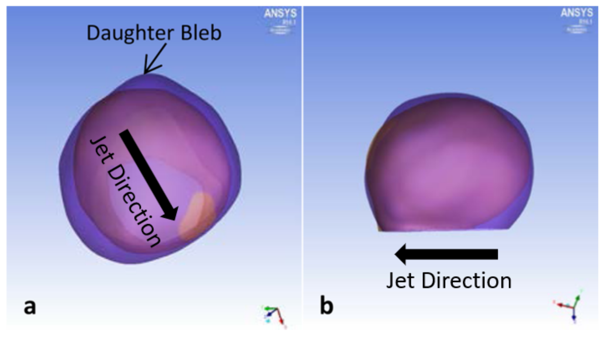
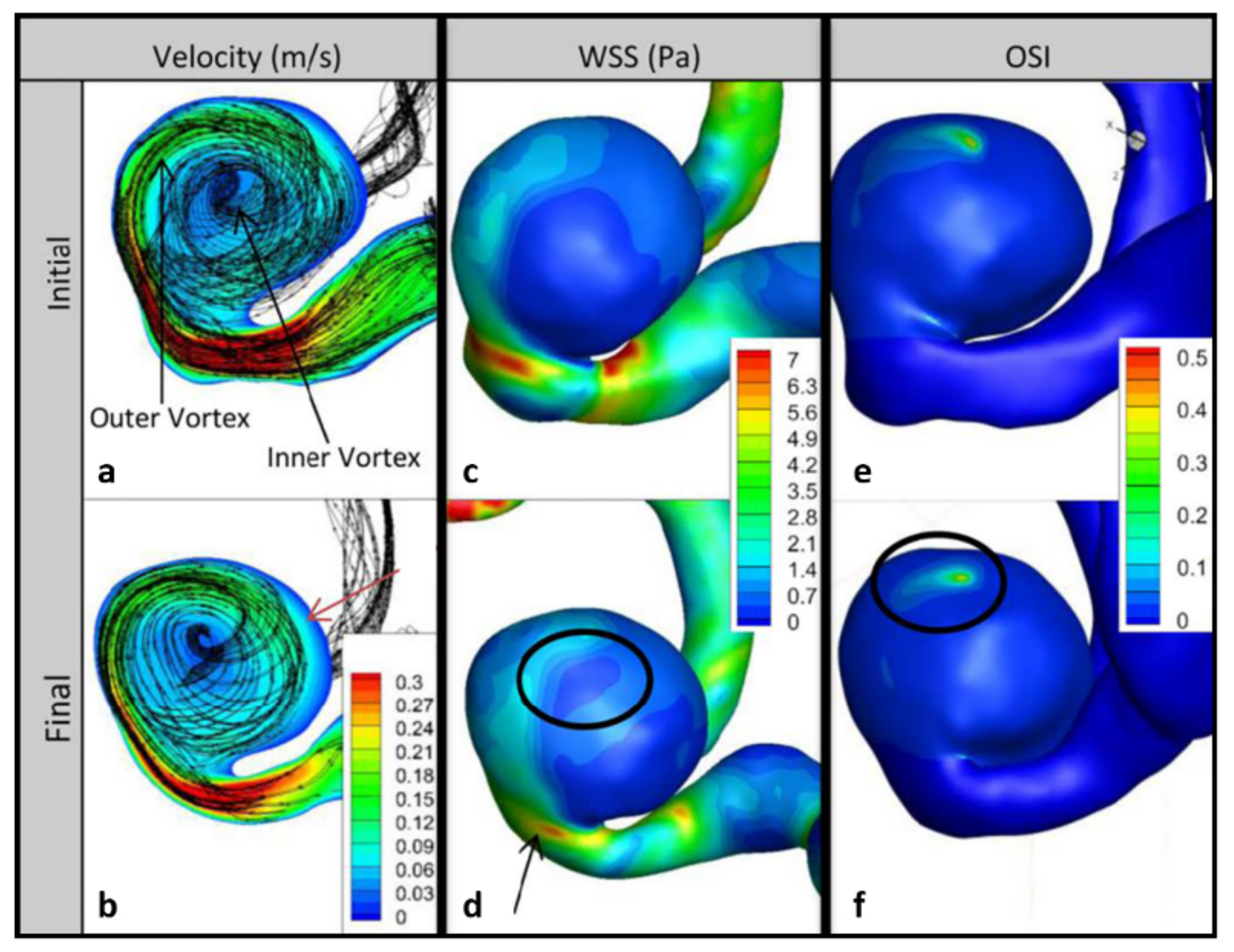
3.1. P1 Aneurysm
3.2. P2 Aneurysm
3.3. P3 Aneurysm
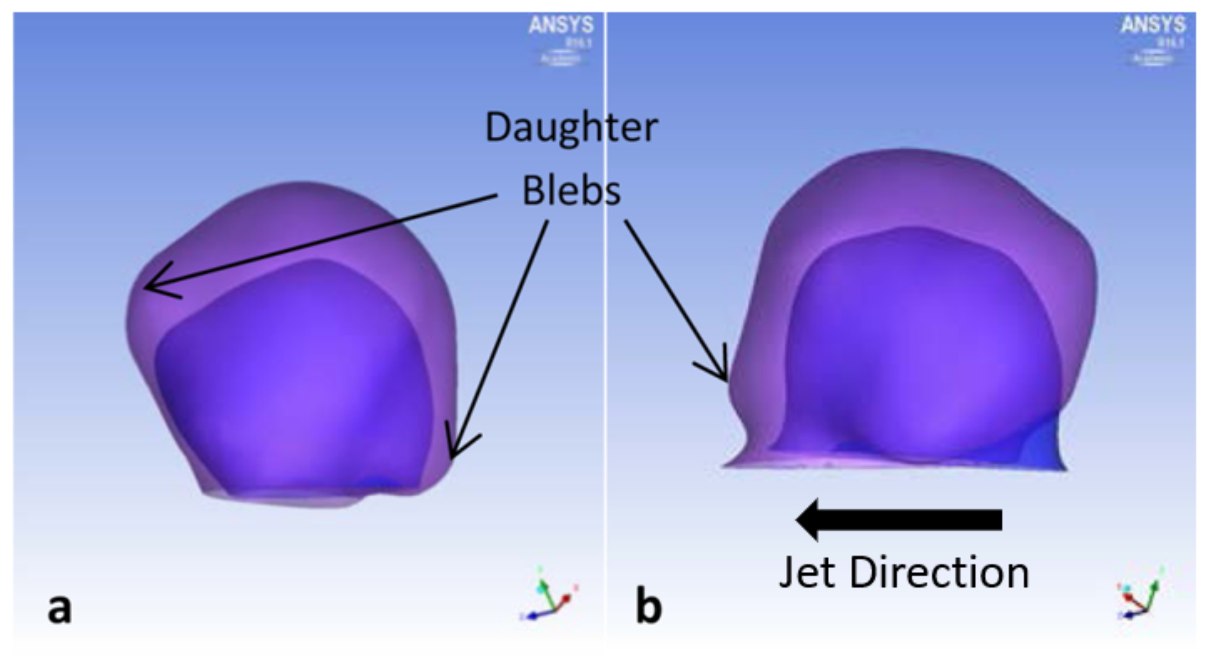
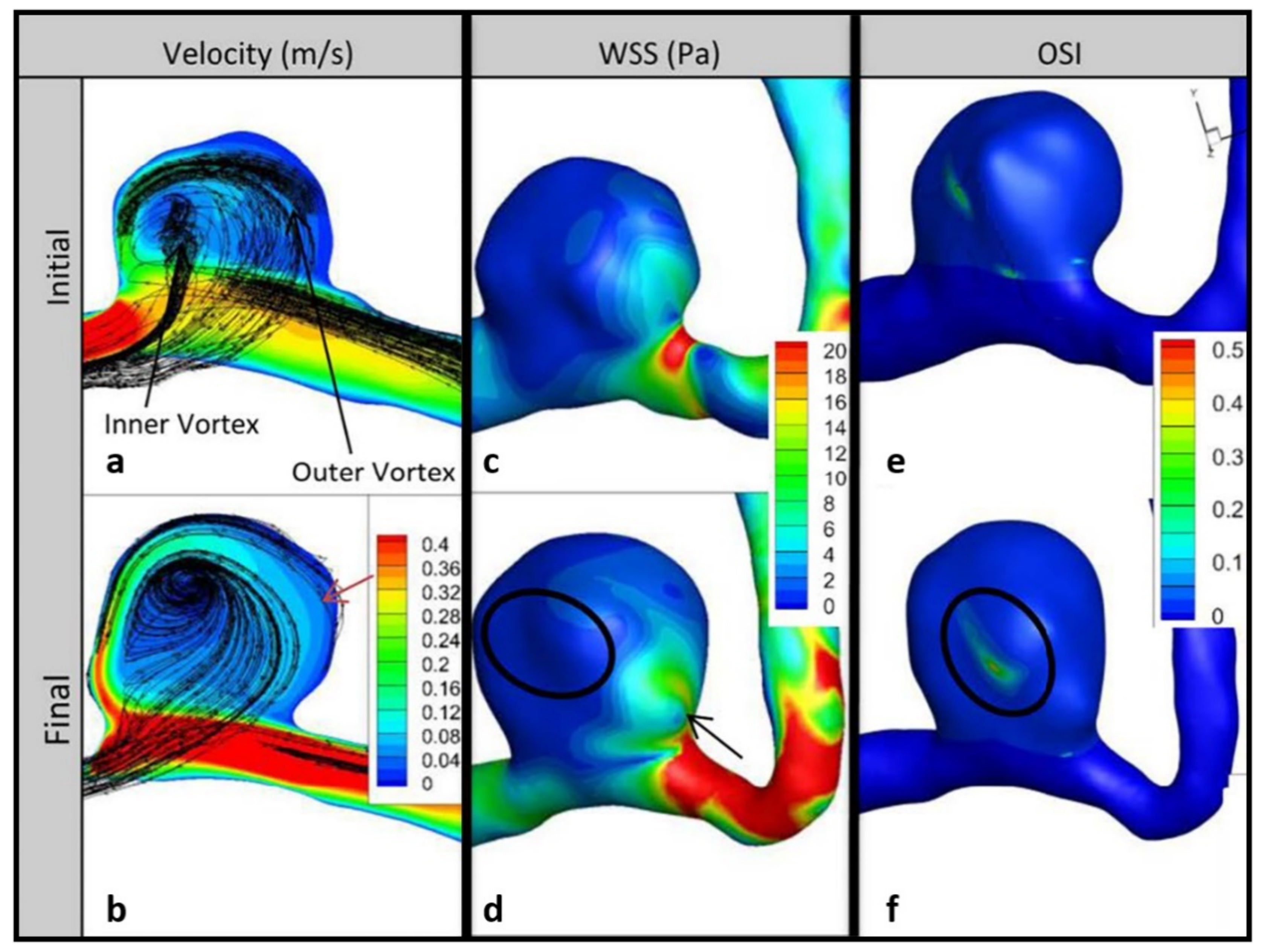
3.4. P4 Aneurysm
4. Discussion
5. Conclusions
Author Contributions
Funding
Institutional Review Board Statement
Informed Consent Statement
Data Availability Statement
Conflicts of Interest
References
- Rinkel, G.J.; Djibuti, M.; Algra, A.; van Gijn, J. Prevalence and risk of rupture of intracranial aneurysms: A systematic review. Stroke 1998, 29, 251–256. [Google Scholar] [CrossRef] [PubMed] [Green Version]
- Cebral, J.R.; Mut, F.; Weir, J.; Putman, C.M. Association of hemodynamic characteristics and cerebral aneurysm rupture. AJNR Am. J. Neuroradiol. 2011, 32, 264–270. [Google Scholar] [CrossRef] [PubMed]
- Berg, P.; Voss, S.; Janiga, G.; Saalfeld, S.; Bergersen, A.W.; Valen-Sendstad, K.; Bruening, J.; Goubergrits, L.; Spuler, A.; Chiu, T.L.; et al. Multiple Aneurysms AnaTomy CHallenge 2018 (MATCH)-phase II: Rupture risk assessment. Int. J. Comput. Assist Radiol. Surg. 2019, 14, 1795–1804. [Google Scholar] [CrossRef] [PubMed]
- Hodis, S.; Kargar, S.; Kallmes, D.F.; Dragomir-Daescu, D. Artery length sensitivity in patient-specific cerebral aneurysm simulations. AJNR Am. J. Neuroradiol. 2015, 36, 737–743. [Google Scholar] [CrossRef] [PubMed] [Green Version]
- Hodis, S.; Uthamaraj, S.; Smith, A.L.; Dennis, K.D.; Kallmes, D.F.; Dragomir-Daescu, D. Grid convergence errors in hemodynamic solution of patient-specific cerebral aneurysms. J. Biomech. 2012, 45, 2907–2913. [Google Scholar] [CrossRef] [PubMed]
- Zarrinkoob, L.; Ambarki, K.; Wahlin, A.; Birgander, R.; Eklund, A.; Malm, J. Blood flow distribution in cerebral arteries. J. Cereb. Blood Flow Metab. 2015, 35, 648–654. [Google Scholar] [CrossRef] [PubMed] [Green Version]
- Miura, Y.; Ishida, F.; Umeda, Y.; Tanemura, H.; Suzuki, H.; Matsushima, S.; Shimosaka, S.; Taki, W. Low wall shear stress is independently associated with the rupture status of middle cerebral artery aneurysms. Stroke 2013, 44, 519–521. [Google Scholar] [CrossRef] [PubMed] [Green Version]
- Xiang, J.; Natarajan, S.K.; Tremmel, M.; Ma, D.; Mocco, J.; Hopkins, L.N.; Siddiqui, A.H.; Levy, E.I.; Meng, H. Hemodynamic-morphologic discriminants for intracranial aneurysm rupture. Stroke 2011, 42, 144–152. [Google Scholar] [CrossRef] [PubMed] [Green Version]
- Boussel, L.; Rayz, V.; McCulloch, C.; Martin, A.; Acevedo-Bolton, G.; Lawton, M.; Higashida, R.; Smith, W.S.; Young, W.L.; Saloner, D. Aneurysm growth occurs at region of low wall shear stress: Patient-specific correlation of hemodynamics and growth in a longitudinal study. Stroke 2008, 39, 2997–3002. [Google Scholar] [CrossRef] [PubMed] [Green Version]
- Sugiyama, S.; Meng, H.; Funamoto, K.; Inoue, T.; Fujimura, M.; Nakayama, T.; Omodaka, S.; Shimizu, H.; Takahashi, A.; Tominaga, T. Hemodynamic analysis of growing intracranial aneurysms arising from a posterior inferior cerebellar artery. World Neurosurg. 2012, 78, 462–468. [Google Scholar] [CrossRef] [PubMed]
- Shojima, M.; Oshima, M.; Takagi, K.; Torii, R.; Nagata, K.; Shirouzu, I.; Morita, A.; Kirino, T. Role of the bloodstream impacting force and the local pressure elevation in the rupture of cerebral aneurysms. Stroke 2005, 36, 1933–1938. [Google Scholar] [CrossRef] [PubMed] [Green Version]
- Cebral, J.R.; Hendrickson, S.; Putman, C.M. Hemodynamics in a lethal basilar artery aneurysm just before its rupture. AJNR Am. J. Neuroradiol. 2009, 30, 95–98. [Google Scholar] [CrossRef] [PubMed] [Green Version]
- Hodis, S.; Uthamaraj, S.; Lanzino, G.; Kallmes, D.F.; Dragomir-Daescu, D. Computational fluid dynamics simulation of an anterior communicating artery ruptured during angiography. J. Neurointerv. Surg. 2014, 6, e14. [Google Scholar] [CrossRef] [PubMed] [Green Version]
- Mantha, A.; Karmonik, C.; Benndorf, G.; Strother, C.; Metcalfe, R. Hemodynamics in a cerebral artery before and after the formation of an aneurysm. AJNR Am. J. Neuroradiol. 2006, 27, 1113–1118. [Google Scholar] [PubMed]
- Tateshima, S.; Tanishita, K.; Omura, H.; Villablanca, J.P.; Vinuela, F. Intra-aneurysmal hemodynamics during the growth of an unruptured aneurysm: In vitro study using longitudinal CT angiogram database. AJNR Am. J. Neuroradiol. 2007, 28, 622–627. [Google Scholar] [PubMed]


| ID | Location | Initial Size (mm) | Final Size (mm) | Initial MRA Year | Final MRA Year | Growth Time (Years) |
|---|---|---|---|---|---|---|
| P1 | ICA dx. | 8 | 9 | 2008 | 2010 | 1.08 |
| P2 | ACom and ICA sin. | 5 | 7 | 2005 | 2011 | 5.96 |
| P3 | MCA dx. | 8 | 9 | 2009 | 2011 | 2.64 |
| P4 | MCA dx. | 0.5 | 2 | 2007 | 2015 | 7.33 |
| ID | Hemodynamic Changes | Morphological Changes | ||||||
|---|---|---|---|---|---|---|---|---|
| WSS | OSI | KE | Volume | SR | AR | EI | NSI | |
| P1 | −27% | −33% | 256% | 61% | 3% | −5% | 36% | −35% |
| P2 | 0% | 9% | 56% | 56% | 2% | 6% | 23% | −12% |
| P3 | −2% | 31% | 7% | 11% | 6% | 0% | 24% | 6% |
| P4 | −3% | 6% | 131% | 170% | 49% | 15% | −11% | −10% |
Publisher’s Note: MDPI stays neutral with regard to jurisdictional claims in published maps and institutional affiliations. |
© 2021 by the authors. Licensee MDPI, Basel, Switzerland. This article is an open access article distributed under the terms and conditions of the Creative Commons Attribution (CC BY) license (https://creativecommons.org/licenses/by/4.0/).
Share and Cite
Nordahl, E.R.; Uthamaraj, S.; Dennis, K.D.; Sejkorová, A.; Hejčl, A.; Hron, J.; Švihlová, H.; Carlson, K.D.; Suzen, Y.B.; Dragomir-Daescu, D. Morphological and Hemodynamic Changes during Cerebral Aneurysm Growth. Brain Sci. 2021, 11, 520. https://doi.org/10.3390/brainsci11040520
Nordahl ER, Uthamaraj S, Dennis KD, Sejkorová A, Hejčl A, Hron J, Švihlová H, Carlson KD, Suzen YB, Dragomir-Daescu D. Morphological and Hemodynamic Changes during Cerebral Aneurysm Growth. Brain Sciences. 2021; 11(4):520. https://doi.org/10.3390/brainsci11040520
Chicago/Turabian StyleNordahl, Emily R., Susheil Uthamaraj, Kendall D. Dennis, Alena Sejkorová, Aleš Hejčl, Jaroslav Hron, Helena Švihlová, Kent D. Carlson, Yildirim Bora Suzen, and Dan Dragomir-Daescu. 2021. "Morphological and Hemodynamic Changes during Cerebral Aneurysm Growth" Brain Sciences 11, no. 4: 520. https://doi.org/10.3390/brainsci11040520