
Elastic Slow Dynamics in Polycrystalline Metal Alloys


1
Institute of Thermomechanics of the Czech Academy of Sciences, 18200 Prague, Czech Republic
2
DISAT, Condensed Matter Physics and Complex Systems Institute, Politecnico di Torino, 10129 Torino, Italy
*
Author to whom correspondence should be addressed.
Appl. Sci. 2021, 11(18), 8631; https://doi.org/10.3390/app11188631
Submission received: 27 July 2021
/
Revised: 10 September 2021
/
Accepted: 13 September 2021
/
Published: 16 September 2021
(This article belongs to the Section Acoustics and Vibrations)
Abstract
:Elastic slow dynamics, consisting in a reversible softening of materials when an external strain is applied, was experimentally observed in polycrystalline metals and presents analogies with the same phenomenon more widely observed in consolidated granular media. Since the effect is extremely small in metals, precise experimental techniques are needed. Reliable measurement of relative velocity variations of the order of is crucial to perform the analysis. In addition, the grain structure and the nature of grain boundaries in metals is very different from that in rocks or concrete. Therefore, linking relaxation elastic effects to the microstructure is needed to understand the physical origin of slow dynamics in metals. Here, interpreting the relaxation phenomenon as a multirelaxation process, we show that it is sensitive to the spatial scale at the microstructural level, up to the point of allowing the identification of the existence of features at different spatial scales, particularly distinguishing damage from microstructural inhomogeneities.
1. Introduction
Slow dynamics is perhaps the most characteristic feature of elastic hysteresis manifested in media with a grain structure [1,2,3,4]. These materials exhibit memory effects and hysteresis in their response even when subjected to a low amplitude dynamic excitation (strain of the order of ). Typically, this occurs in rocks [5,6,7,8], concrete [9,10], mortar [11] or unconsolidated granular media [12]. The phenomenon of slow dynamics consists in the existence of equilibrium states of the material, characterised by given viscoelastic properties (modulus [13] and damping [14]), which are dependent on the strain applied to the material. The relaxation to such equilibrium state is a long-time relaxation process, similar to other phenomena unrelated to the field of elasticity [15,16,17,18].
More specifically, slow dynamics effects consist in a conditioning and a relaxation phase. Given a fully relaxed sample (with unperturbed values of modulus and damping), an external perturbation is applied producing a strain. This phase is called conditioning and the conditioning strain could be generated with a propagating elastic wave [19], by heating/cooling a sample [20,21] or with an impact [22]. As a consequence, microstructural reorganisation occurs and wave velocity changes in time, following the change in time in modulus which evolves towards its new equilibrium value [23,24]. The physical mechanisms taking place are still unclear: fluids redistribution [7,25], sliding, adhesion and/or friction [26,27,28], dislocations rearrangement [29] or clapping surfaces in cracks [30], etc. As soon as the conditioning excitation is removed, the system relaxes back, which means that the modulus recovers slowly to its original unperturbed value [31,32]. The process can be monitored by tracking the evolution of wave velocity in time using a very low amplitude excitation.
Relaxation was studied extensively in consolidated granular media or damaged composites. Much less attention was devoted to the behavior of polycrystalline metals and metal alloys. Some evidence of hysteresis was shown in [29] and slow dynamics was observed in sintered steel [33], metal alloys [34,35] and metal monocrystals [36]. More recently, slow dynamic effects were observed in metallic spheres [37]. The reason for the limited attention to elastic hysteresis in metals is mainly due to the fact that effects to be measured are much smaller than in consolidated granular media. Velocity variations of the order of must be detected to fully capture the details of the relaxation curve.
In order to study metallic alloys, two main problems should be considered. First, an experimental set-up with high sensitivity and reliability is needed. Standard approaches extracting velocity evolution monitoring the dependence of the resonance curve on time [38,39,40] have to be revised, as shown in Section 3, to make them suitable for studying metals. Here we will discuss an efficient approach based on a semi-analytical inversion (MoDaNE approach) [41,42], which is an alternative to the more difficult to implement Dynamic Acoustoelastic Testing approach used efficiently by other authors for studying early times relaxation in rocks [43].
The second issue is that of developing efficient post-processing tools which allows modelling the behavior and extracting quantitative information. Indeed, as we will discuss in the next section, the qualitative behavior of polycrystalline alloys looks very similar to that of consolidated granular media, even though the boundaries between grains have very different properties than in concrete or rocks. The long time nature of the relaxation process, suggests to study it as a multirelaxation process [44,45]. Previous attempts to apply this approach for the interpretation of experimental data were based on using a discrete basis of relaxation times [43] or by introducing a lower and upper cut-off for relaxation times [37]. As discussed in Section 4, our aim here is to go beyond such approaches in order to derive a continuous distribution of relaxation times and link it to specific features (e.g., grains size) of the materials tested, either in their intact or damaged state, as discussed in Section 5. For the sake of completeness, we mention here that other approaches for interpreting the experimental observations in rocks have also been proposed [46,47,48], which however present some limits which will not be discussed here.
2. Relaxation Process
We show here a typical result of a slow dynamics experiment, to summarise the observed phenomenology and to highlight the questions which we aim to discuss in this paper. In these experiments (see Section 3), the propagation velocity is measured in the relaxed sample (preconditioning) using a low amplitude probing wave. After conditioning, induced using a high strain perturbation, the same low amplitude probing is used to monitor in time the evolution of wave velocity (during relaxation).
A plot as a function of time of the relative velocity variation
describes the evolution of the system properties during the relaxation phase and normalizes the velocity variation with respect to differing material properties as in [33]. Since we are considering longitudinal resonances, the relative velocity variation corresponds exactly to the resonance frequency variation used to monitor slow dynamics in previous works [33]. Note also that analogous considerations could be made for the evolution of damping [14].
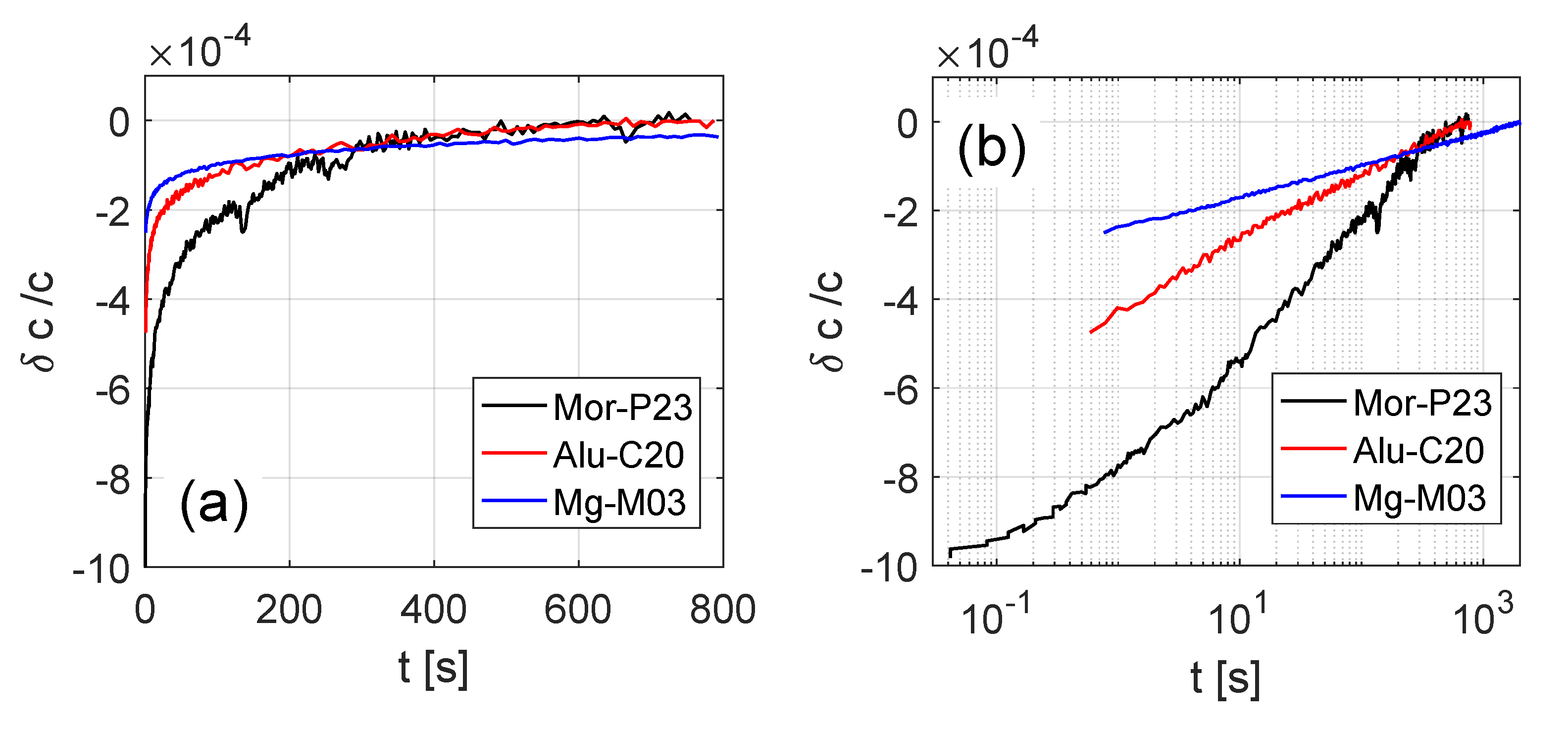
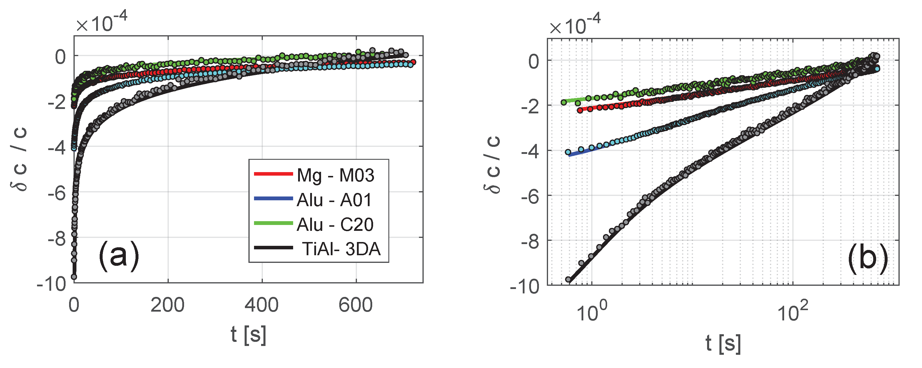
Typical observations are reported in Figure 1 for two metallic samples (Al and Mg based alloys, see Section 3.1) and for a consolidated granular material (mortar). The main features of the relaxation process could be summarised as follows:
- immediately after conditioning, velocity drops of a quantity and an initial not logarithmic in time relaxation occurs for a short time;
- afterwards, in the intermediate time range, the modulus evolves logarithmically with time: ;
- finally, more slowly, velocity relaxes back to its relaxed value: .
From the qualitative point of view, strong similarities in the behavior are present, despite the intrinsic different nature of the grain contacts between consolidated granular media (in which the volume between grains is occupied by a consolidating material) and metal alloys (in which there is no loose contact between grains, since the grain boundary in polycrystalline materials is formed by the mismatch between neighbouring crystal lattices). The main features of the relaxation process, which are those normally considered in the literature, i.e., its logarithmic behavior at intermediate times and its long duration in time, are manifested by all samples considered. In all cases full relaxation occurs and, from a qualitative point of view, the duration of the relaxation process is comparable.
The definition of the time at which relaxation starts () is crucial in view of understanding the evolution and identifying the transition to the logarithmic phase. In our approach, we define as the time corresponding to the switching off of the conditioning amplitude. Electronics delays are negligible, but reverberation of the conditioning phase takes place, during which conditioning and relaxation are mixed-up. This means that the effective initial time of relaxation could be any time between , where is the reverberation time, which is of the order of tens of milliseconds. However, a time shift of the order of magnitude of seconds does not affect the analysis presented here and thus the choice adopted for allows to consider our results reliable and robust.
Moreover, the definition of the equilibrium velocity (i.e., the value of velocity at ) is important. As given in Equation (1), the equilibrium velocity at the end of the relaxation process was estimated by the value of wave velocity measured before conditioning , which corresponds to the expected full recovery. This hypotheses was verified to avoid inconsistencies in our fit due to the presence of an unknown offset with respect to . For all datasets, a preliminary fit was performed considering an additional free offset parameter in the fitting function, which was indeed found to be close to zero (with relative values of the order of ).
3. Materials and Methods
3.1. Samples
Several intact metallic alloy samples have been considered in our studies. Specifically, we have analysed:
- a 3D printed titanium-alloy (sample TiAl-3DA): A prismatic sample of dimensions mm was fabricated by Electron Beam Melting technology using optimal process parameters. The microstructure consists of fine lamellar Widmanstatten morphology with columnar grains extending over multiple build layers. The typical reported lath length is approx. 20 m and width in the range m–4 m [49]. Columnar grains size can reach multiple millimeters in length [50];
- an aluminum alloy specimen (sample Alu-C20): A prismatic sample of dimensions mm was manufactured from a rolled sheet of D16CT1 alloy (Al-4Cu-1Mg) with anisotropic microstructure and average grain size around 400 m [51]. The microstructure also contains dispersed tubular precipitates;
- a second aluminum alloy specimen (sample Alu-A01): A cylindrical sample was taken from a cold drawn round bar of 7075 Al alloy (Al-4Zn-2Cu). The microstructure is strongly anisotropic with typical grain size 80 m in transverse and up to 1.5 mm in longitudinal direction. Small intermetallic precipitates of AlFe and MgZn are dispersed in the matrix. The sample had length 120 mm and diameter 12 mm.
- a magnesium composite specimen (sample Mg-M03): A prismatic specimen was machined from a squeeze cast magnesium AX41 alloy (Mg-4Al-1Ca) reinforced by 12% Saffil fibres ( alumina). The microstructure contains equiaxed grains with typical size 90 m, traces of intermetallic phase MgAl at grain boundaries and small AlCu precipitates. The fibres have a planar random orientation with respect to the squeezing direction. The sample dimensions were 135 × 20 × 13 mm.
The first three samples were also analysed inducing microstructural changes (damage) as discussed in Section 5.
In addition, we have also considered data relative to a consolidated granular sample as a reference for the discussion. Data refer to mortar (sample Mor-P23), in the shape of a prism ( 160 mm), produced using Portland cement. Sand grains are in the range 0 to 2 mm size [52]. Details about data acquisition for this sample are reported in ref. [24].
3.2. Experimental Set-Up
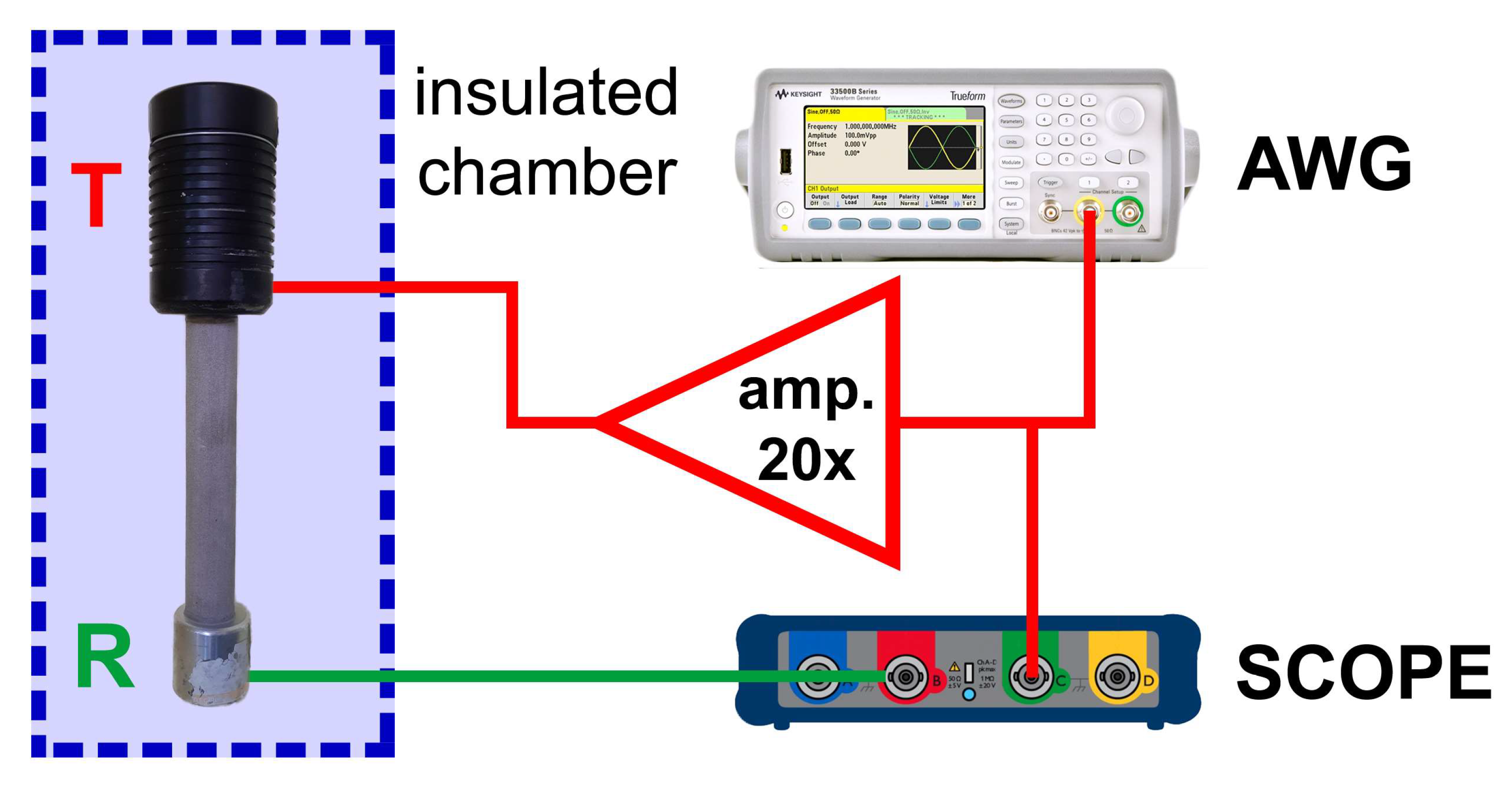
The experimental set-up (see Figure 2) consists in an Agilent 33500 arbitrary waveform generator, connected to a voltage amplifier (FLC F20A ×20). Signals were transmitted into the sample by a PZT actuator (IMG, with resonance frequency 27 kHz), glued to one end of the sample using cyanoacrylate. Output signals were detected by a PZT transducer (Matest C370-02) glued to the other end of the sample. Transducers work dominantly in longitudinal configuration. Detected signals were recorded as waveforms (voltage vs. time) by a Picoscope 6402C oscilloscope at the sampling frequency of 40 MHz.
All measurements were performed in an insulated chamber in order to minimise the effects of environmental fluctuations (e.g., temperature or humidity). The experimental setup was tested for linearity and it was shown that changing configuration or means of conditioning did not alter the relaxation curve significantly (as reported in Appendix B). In particular, two experimental configurations were adopted:
- Suspended. Samples were vertically suspended on thin nylon filaments: Mg-M03, Alu-A01 and Ti-Al-3DA were tested in this configuration;
- Horizontal. Samples were placed horizontally on a foam layer: Mor-P23, Ti-Al-3DA and Alu-C20 were tested in this configuration.
Equivalent results have been obtained for the Ti-Al-3DA sample in both configurations.
3.3. Measurement Protocol
Except for the mortar sample, the measurement procedure was implemented with the following protocol:
- pre-conditioning: The sample was excited by a low amplitude () 30 ms-long chirp with a frequency linearly varying in a narrow range around one longitudinal mode. The chirp was repeated and the acquired waveforms were post-processed by discrete-time Fourier transform (DTFT) to obtain the resonance curves at successive times . The duration of the chirp excitation was chosen as the shortest one guaranteeing results independent from the length of the chirp;
- conditioning: The source was switched to a sinusoidal wave with frequency slightly above the monitored resonance frequency and amplitude to induce conditioning (this phase was not monitored here) up to a new equilibrium elastic state. Duration of conditioning was in the range of 3.5 min;
- relaxation: The source is again the chirp function used in the pre-conditioning phase. The sample is probed in defined time intervals, which allows us to obtain a time evolution of the resonance curve .
Each sample was tested repeatedly while decreasing the conditioning amplitude . Details about the frequency ranges used for the various samples and the typical input amplitude voltages are reported in Appendix A.
3.4. Data Analysis
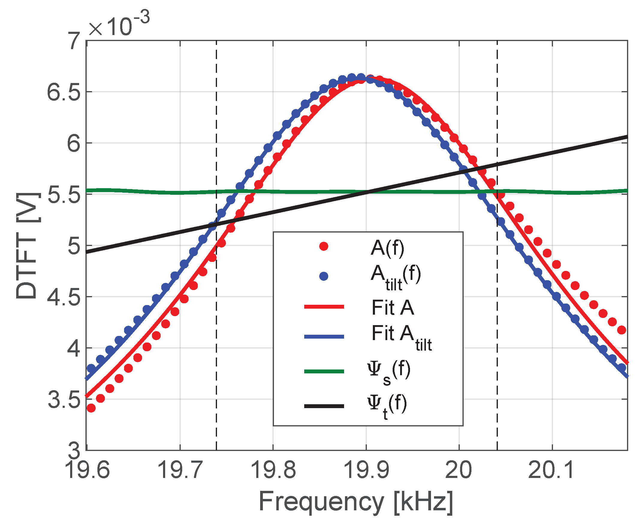
For each waveform recorded at time t as mentioned above, the corresponding propagation velocity in the sample can be derived using a semianalytical formulation (MoDaNE) described in ref. [41,42]. As already mentioned, each acquired waveform was post-processed by discrete-time Fourier transform with 2 Hz resolution to obtain the resonance curve; an example of results is shown in Figure 3 (red symbols).
In the MoDaNE approach, the displacement solution in (i.e., at the receiver position) was found for a sinusoidal forcing in . The amplitude of the solution as a function of frequency is expressed as
where L is the sample length, is the source amplitude (after proper calibration), is the damping factor and k is the wavenumber, , being c the wave velocity. By fitting the experimental results (either or ), the wave velocity can be derived (together with the other parameters and ).
The fit result for the raw experimental data in Figure 3, shown as a red line, is not optimal, due to the distortions induced by two sources of error, which need to be corrected:
- the transducers frequency response, which is not completely flat in the frequency range considered. A tilting correction to experimental data could then be obtained by dividing the experimental resonance curves with the transducer response , shown as a black line in Figure 3;
- the source function distortions, which is not a perfect square function in the frequency domain. The corresponding deconvolution is given by the DTFT of the source signal (green line).
The resulting tilted resonance curve can be obtained
and it is shown as blue symbols. Here, the symbol A denotes the amplitude of the DTFT for each frequency . The fit of the tilted resonance curve (blue line) is significantly improved.
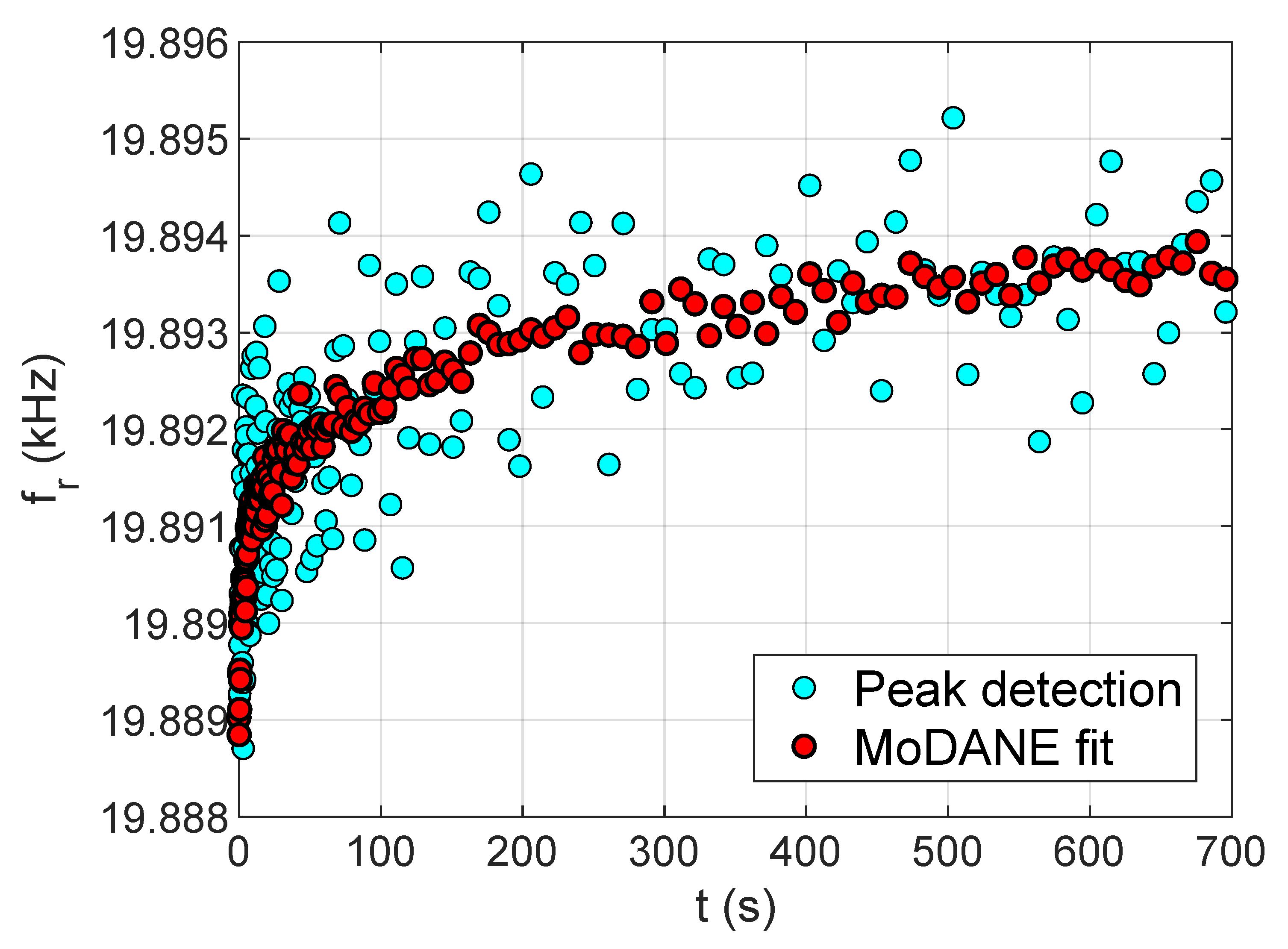
The procedure discussed above is applied to signals acquired at different times during relaxation. It follows that curves of velocity vs. time could be derived as shown in Figure 4, where we plot resonance frequency (proportional to velocity) vs. time. Figure 4 allows also to appreciate the correctness and accuracy of the approach proposed. Here, the relaxation curve of velocity for sample Alu-C20 is derived using the MoDaNE approach (red symbols) and compared with that obtained deriving velocity from the peak of the resonance curve (cyan symbols), obtained from a parabolic fit around the maximum. The two approaches provide the same result, but fluctuations are significantly smaller when MoDaNE is applied, indicating a higher accuracy in the determination of velocity.
4. Multi-Relaxation Theory and Results
During relaxation, propagation velocity in the sample varies with time up to its equilibrium value (corresponding to that before conditioning): See results shown in Figure 1. As already discussed, the behaviour is not a simple exponential and, as for many other systems [15,16,17,18], it can be described as a multi-relaxation process with relaxation times :
where is the relative velocity variation defined in Equation (1). Determination of the function (called from now on relaxation times distribution) allows to analyse and quantify relaxation effects and compare the behaviour of different solids.
4.1. Theory
Inversion of experimental data to derive the unknown distribution is made difficult by the non-uniqueness of the solution, further complicated by the big span of relaxation times needed to describe both early and late times of the evolution (from at least s to s). Experimental [43] and theoretical [37] attempts have been reported in the literature to characterise the function and we will show here that our approach is consistent with these results, but gives a more complete picture.
The proposed procedure was to:
- fit experimental data with a finite/discrete basis of exponentials logarithmically spaced in relaxation times, as in ref. [43];
- shift the fitting basis to obtain an estimate of a continuous distribution in the space and derive an approximate distribution in the linear space;
- guess a suitable analytical expression with a limited number of parameters for the continuous relaxation times distribution and determine its parameters by fitting again the experimental data in continuous space of relaxation times.
4.1.1. Discrete Relaxation Times Distribution in the Log-Space
As a first step, to derive in a rough approximation the main properties of the function , we approximate the solution as a finite sum of exponentials. To this purpose a basis of relaxation times should be defined. Since the basis must span a large time interval, it is more practical to work in a log space. Therefore the basis is defined as a vector where . The elements of the basis are equally spaced with spacing and different basis could be chosen, varying its dimension N or its upper and lower limits and .
In this framework, the fitting function becomes:
where the coefficients could be derived fitting the experimental data.
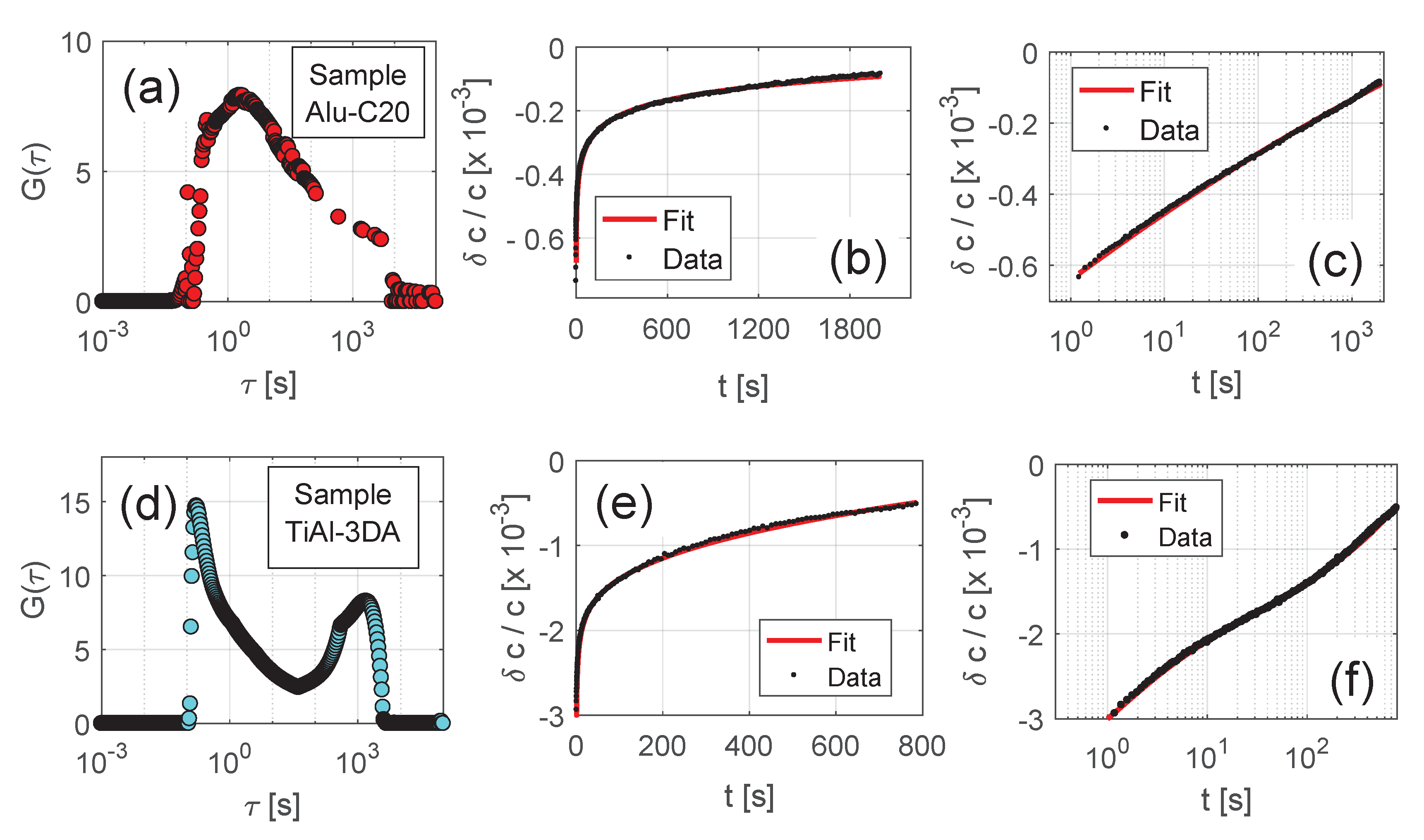
Since the goal is to derive continuous distributions, the fitting procedure can be repeated K times changing the starting point of the basis with . The procedure was applied with and results are shown in Figure 5. For both materials considered we obtain a pseudo-continuous distribution. Thus, the assumption that
is valid.
From results of Figure 5 it could be deduced that:
- in both cases a continuum distribution is found;
- in the case of the Aluminum sample (Alu-C20) shown in subplot(a) the distribution presents a well defined peak and a marked asymmetry with a steep increase for low values of the relaxation time . The same behaviour was also obtained for the other Al sample and for the Magnesium samples (not reported for brevity);
- in the case of the Titanium alloy sample the distribution presents two peaks for different values of preserving the marked asymmetry in the distribution for both.
To obtain the continuous distribution in Equation (4) one more step is needed. Substituting , we obtain:
It follows
where . The resulting distribution could be reasonably well approximated by a distribution with upper and lower bounds in the integration domain, in agreement with the discussion in [37].
However, the use of the fitting procedure in the log-space to derive a continuous distribution in the lin-space is biased by several approximations which make it unreliable, as further proven in the Supplemental Material:
- the distribution of the basis used for the discrete fit is not equally spaced in the linear space;
- the basis elements do not correspond to the central point of the interval in the linear space, e.g., assuming , the element represents the interval , which means that in the linear space represents the interval , whose central point is not ;
- the procedure of dividing by when deriving the distribution in the lin space might amplify errors present in the estimation of the s, especially for low values, thus leading to distortions and/or to a limitation to the definition of details of the distribution .
As a consequence, the procedure described so far could only be reliably used as a qualitative indication of the properties of the underlying continuous relaxation spectrum . As such, as shown in the next Subsection, it could suggest a plausible analytical expression for .
4.1.2. Continuous Spectrum of Relaxation Times
Distributions obtained in the space are continuous (see Figure 5) and suggest in most cases (see subplot (a)) a peaked distribution with asymmetry, i.e., a faster increase of the curve at lower values of (the presence of semilog x-axes should not be misleading). Several choices of peaked and asymmetric functions are of course possible, but they are largely equivalent regarding the uniqueness of the solution, as we show in the Supplemental Material.
In the following, we assume a Weibull distribution of the inverse of relaxation times, which has the expected asymmetry discussed above. This choice is plausibly suggested by the fact that Weibull distribution is typically observed as the most typical distribution of the size of the features present at the grain and crack scales [53,54]. Thus, defining we write:
For the titanium sample, which has a two peaks distribution (see Figure 5d), the relaxation times distribution is the superposition of two Weibull distributions: .
The parameters of the distributions are then obtained fitting the curve in the time domain, integrating in the full space (from zero to infinity) using Equations (4) and (9). Results of the fit for a few cases are shown in Figure 6. The quality of the fitting function (continuous line) in describing the experimental behavior (dots) is evident, with good agreement also for the early stages of the evolution (see subplot (b) where a log time scale is used). In all cases, also the intermediate times logarithmic recovery is obtained. In the case of the Titanium alloy sample (black curve) the need to fit the data using the superposition of two Weibull distributions is particularly evident in subplot (b), where, after a first logarithmic in time phase and a bending at early times (arising from the “saturation” of the first distribution), at about 10 s velocity starts evolving rapidly again with a second logarithmic in time phase.
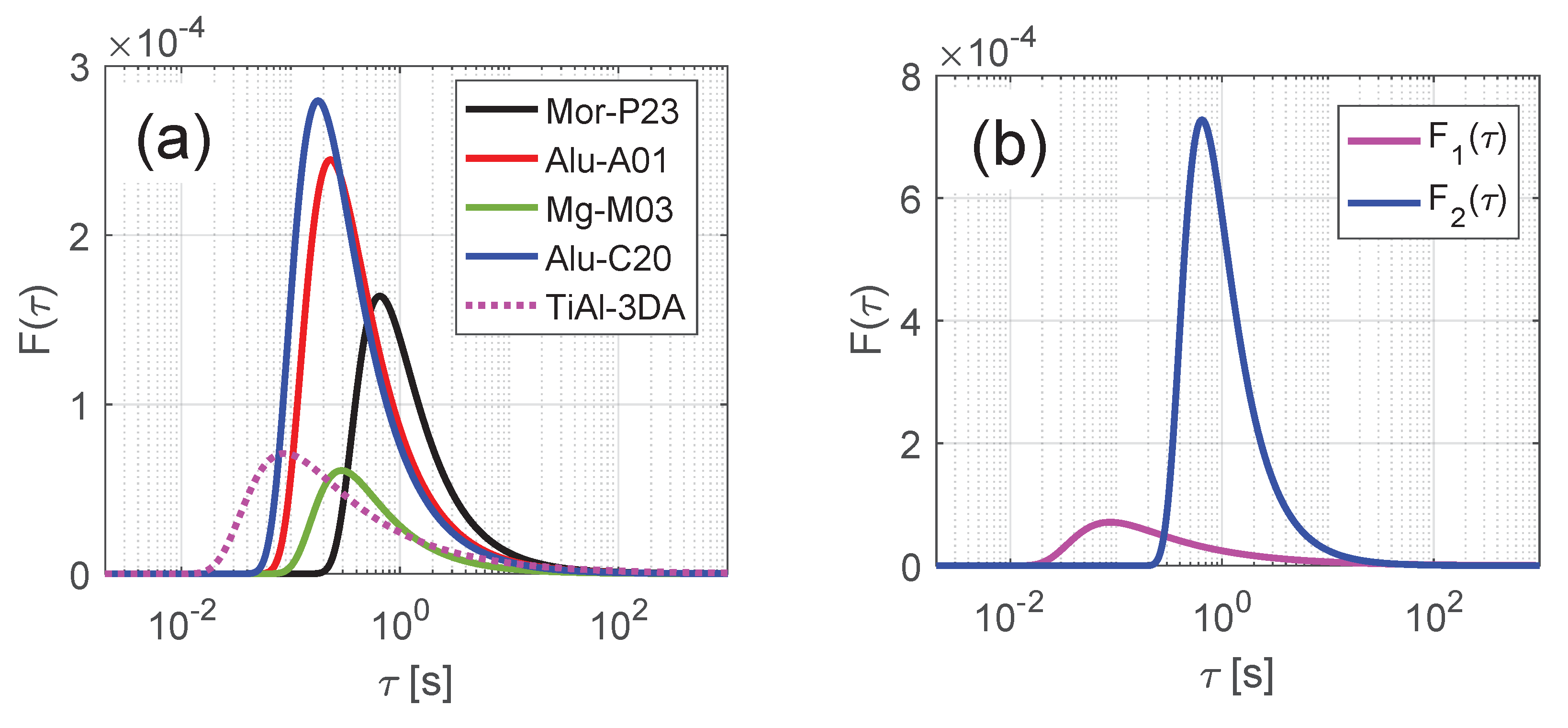
The obtained best fitting distributions for the samples considered are shown in Figure 7. The distributions for the three metal alloys (Aluminum A and C samples and magnesium sample) reported in Figure 7 present a peak at s, which is remarkably similar for the three samples, corresponding to their similar grain size (≈0.1 mm). The peak for mortar ( s) is slightly higher, corresponding to a larger grain size (≈0.8 mm). The two peaks in distribution for the Titanium alloy sample could be linked to the presence of grains with different sizes in this sample: Besides the very small structural grains (size mm, corresponding to the peak at s), the columnar grain structure presents a larger grain size of ≈1 mm (resulting in a second peak at s, i.e., close to the peak of mortar which has a similar grain size).
Besides the link of the peak position to the grain size, intact metal alloys and mortar have a very similar behavior.
4.2. Results and Discussion
4.2.1. Distribution Properties
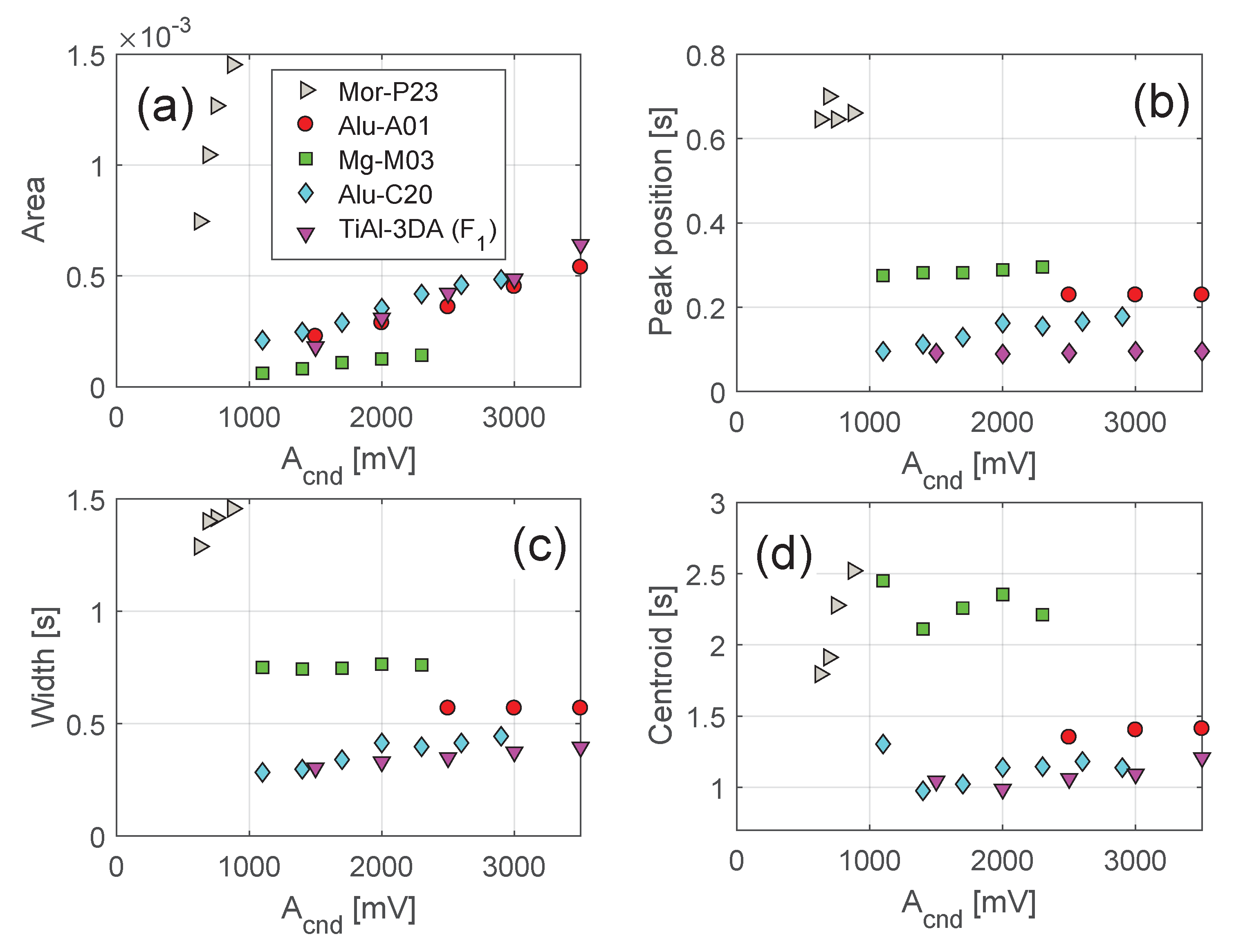
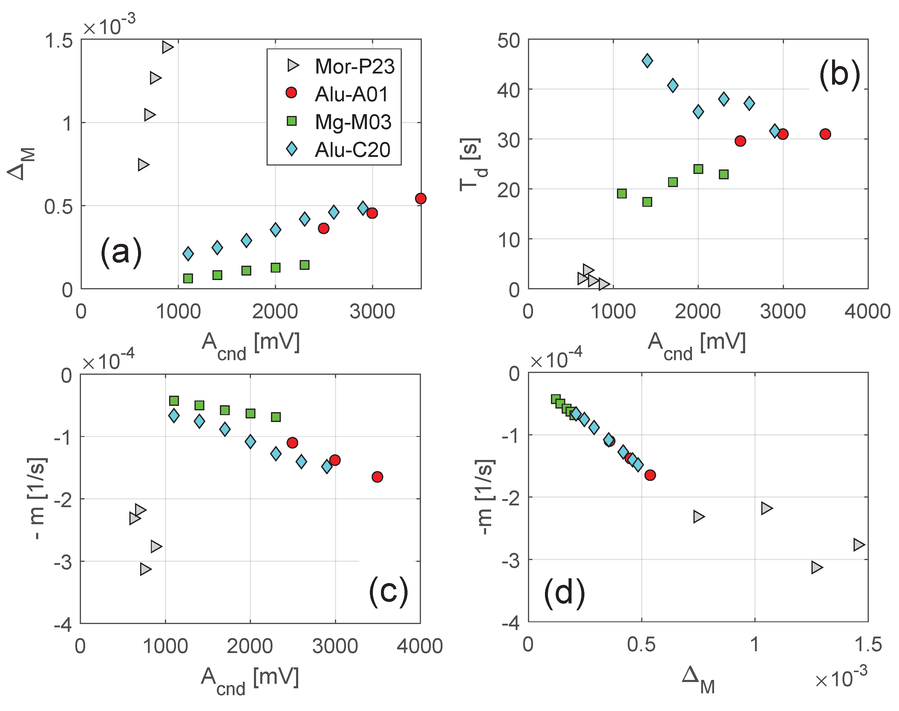
In order to compare properties of the obtained distributions as a function of conditioning amplitude , we introduce the following indicators:
- Area, defined as . It is equal to the velocity variation at time , i.e., it quantifies the amount of conditioning;
- Peak position, defined as the relaxation time corresponding to the maximum of the distribution. It defines the most relevant relaxation time in the process and, as shown above, it is linked to the grain size;
- Width, defined as the width at half height of the distribution;
- Centroid, defined as . It allows to quantify the asymmetry of the function.
The four indicators were calculated for the tested samples at increasing conditioning amplitude in successive experiments and are shown in Figure 8. The area (subplot (a)) for all samples increases linearly with increasing conditioning amplitude. Even though an exact comparison between samples is critical (given that, for the same input, the strain in the sample could be different), still data allow to appreciate that mortar exhibits stronger conditioning than metal alloys, as expected: The area is much larger at lower conditioning amplitude levels. All metal alloys behave similarly, also from a quantitative point of view. Conditioning is weaker in the Magnesium sample. Remarkably, for all samples a threshold for activation of conditioning is present: The fitting straight line intersects the x-axes at a positive value of . The existence of a threshold for conditioning, shown elsewhere for granular samples [24], is thus present also in metal alloys.
The other three indicators are independent from , which suggests that, once the activation threshold is reached, features corresponding to all relaxation times are activated and the number of them participating to relaxation is proportional to the level of conditioning (linear dependence of the area on ). As already discussed, the peak position increases with the grain size. Width and centroid have almost the same value for all metal alloys samples considered, except for the centroid in the case of the composite Magnesium sample, which is slightly larger (i.e., stronger asymmetry) and close to that of mortar.
4.2.2. Relaxation Curve Properties
An additional set of indicators could be introduced starting from the curve representing the velocity variation vs. time (see Figure 1). We introduce the jump , defined as the velocity variation at time , which quantifies the amount of conditioning. As remarked this quantity is equivalent to the area defined above and the same considerations reported above apply. We also consider the time at which half relaxation occurs: is the time at which . Finally we introduce the slope m defined as the slope of the curve in the logarithmic phase of recovery (slope of the straight line fit around in the logarithmic space: ).
The parameters are shown as a function of conditioning amplitude in Figure 9. We observe that relaxation is faster for mortar (subplot (b)) than for metal alloys, albeit this was not evident from a qualitative examination of the evolution curves in Figure 1. The main result here is shown in subplot (d): For all metal alloy samples a linear correlation is found between and m, with the same correlation coefficient for all samples. This linear correlation is approximately valid also for mortar (for which data are noisier), but with a different correlation coefficient.
5. Effects of Variation of the Microstructure
5.1. Distributed Damage
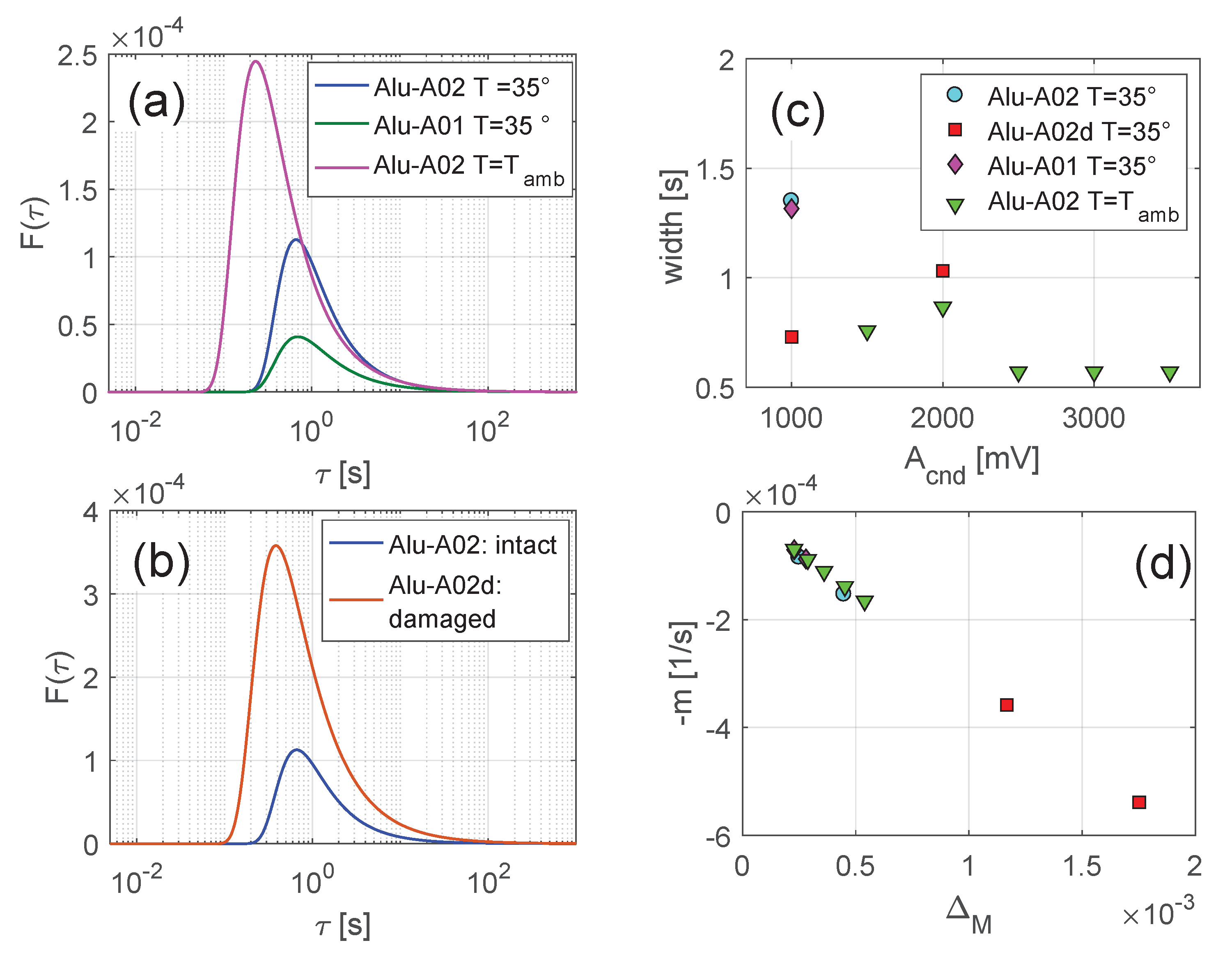
Effects of temperature and distributed damage were analysed on the Aluminum sample (Alu-A01). Three samples with identical geometry and properties were considered. Samples Alu-A01 and Alu-A02 are intact. The former has been tested at room temperature and at a controlled temperature equal to 35 degrees. Results reported in Figure 10 indicate a shift of the distribution towards higher relaxation times for higher temperature (compare pink and green curves in subplot (a)). The variation is not a fluctuation, since repeating the measurement on an identical sample at the higher temperature the same distribution is found (compare blue and green curves). Note that the shift is not incompatible with establishing a link between relaxation times and grain sizes, rather it seems to suggest that grains of the same size relax faster at ambient temperature, i.e., confirming the role played by thermal effects during relaxation.
Sample Alu-A02 was then damaged (the damaged sample labelled as Alu-A02d), by treating it with a droplet of gallium, which is known to interact with aluminum producing distributed disgregation at the grain boundaries [55]. The resulting distribution of relaxation times is identical to that of the intact sample, except in magnitude. As expected, slow dynamics is almost one order of magnitude higher in the damaged sample than in the intact one. The peak position and width are however not influenced by the damage, which thus could be assumed simply to enhance the density of defects already present at the grain boundaries of the intact sample, but not inducing cracks or other features with different space scale.
In subplot (d), the parametric plots of slope m vs. jump are shown for the studied samples, where we recall that the two parameters describe the evolution of velocity vs. time during relaxation. The linear correlation between the two parameters found for intact samples is also maintained in the case of damaged samples and the correlation coefficient is not affected by the presence of damage or by changes in temperature.
5.2. Cracks
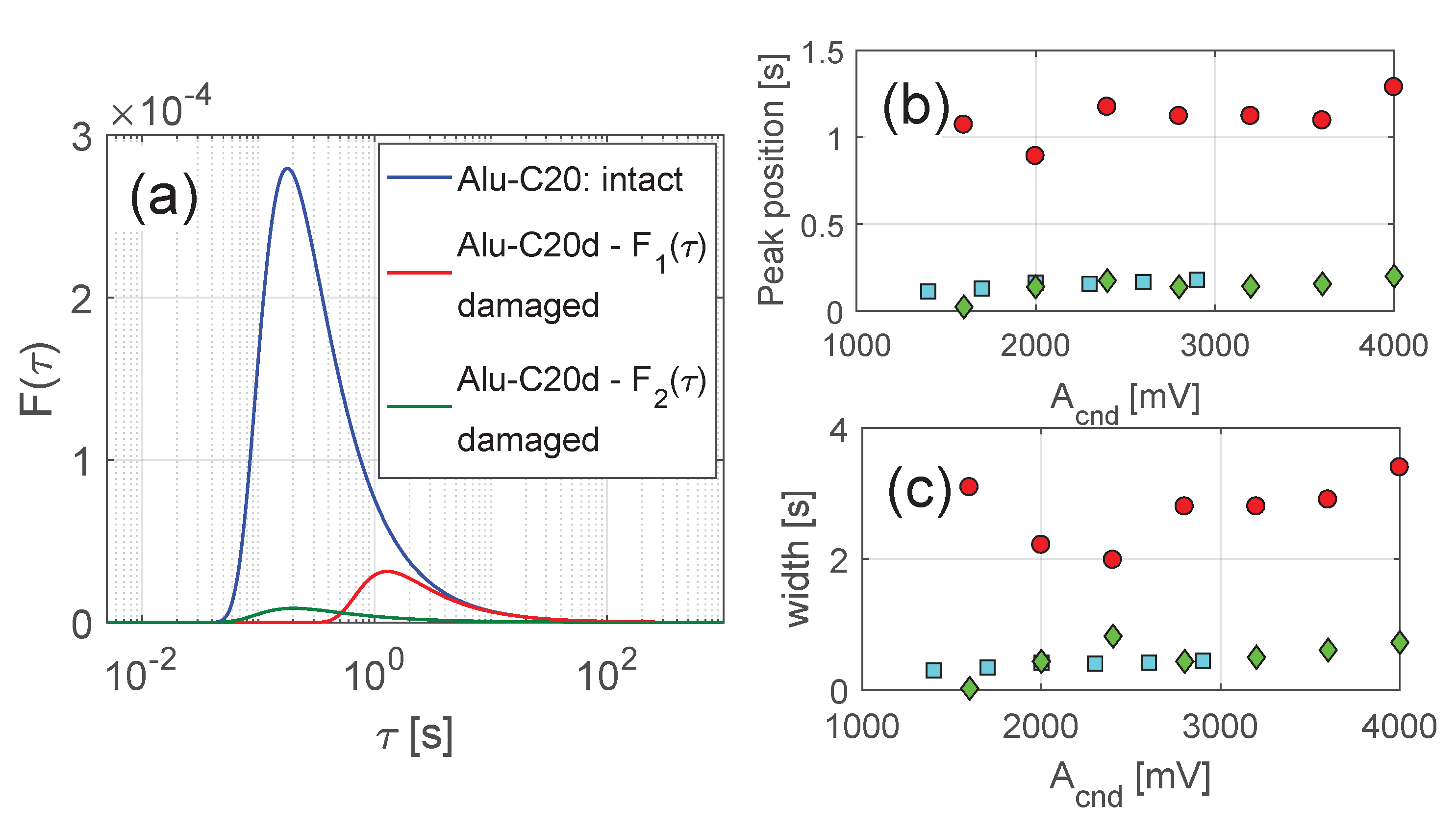
We have also studied effects on the relaxation times distribution due to the presence of a crack. A second sample, identical to the sample Alu-C20, was machined from a larger fatigue test specimen (CT type). A crack was produced in the centre of the sample by fatigue loading with a constant load cycle. The resulting macrocrack was a 10 mm long, with the tip closed due to the stresses resulting from the fatigue process. The portion of the crack whose faces are in partial contact was estimated to be 1 mm long.
The analysis of the relaxation data using a discrete fitting indicated that the damaged sample exhibited a relaxation process characterised by a double peak distribution, similar to that observed for the Titanium Alloy sample (see Supplemental Material for further details). Thus the relaxation times distribution was chosen as . Results of the analysis are reported in Figure 11.
As expected, the two peaks of the damaged sample correspond to different length scales of the microstructural features. The lowest peak is at the same value as that of the intact sample, reasonably since the underlying material grain size is not modified by the presence of a localised crack. The second peak (red dots in subplots (b) and (c)) is found at a higher value of , comparable to the position of the peak for mortar. The result is reasonable again, given that the size of the portion of closed crack is comparable to the grain size in mortar (of the order of 1 mm).
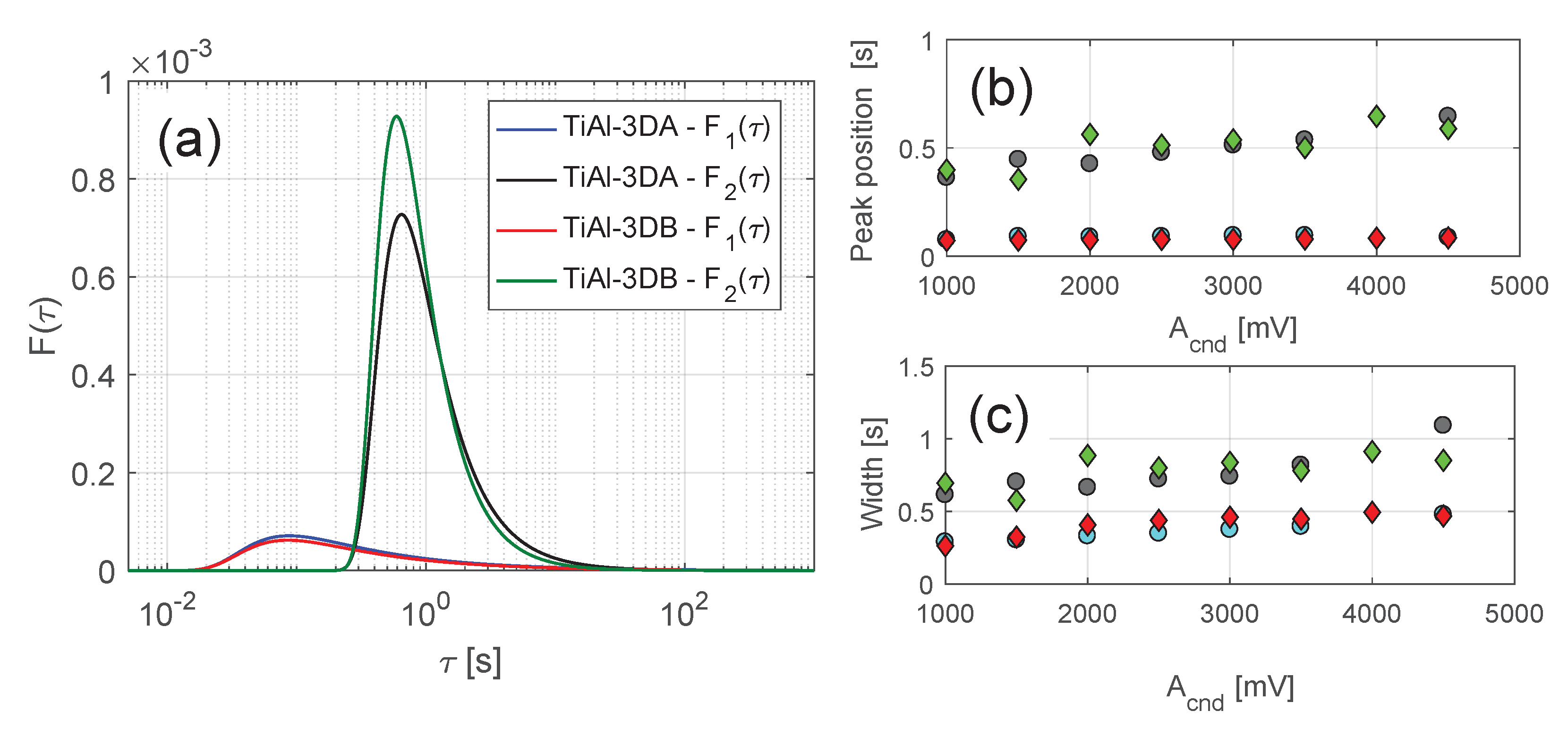
5.3. Porosity
We have analysed the influence of porosity on the relaxation process by considering two Titanium alloy samples fabricated by Electron Beam Melting. One was fabricated using optimal process parameters (TiAl-3DA) and one with an enclosed volume containing imperfectly melted material resulting in volumetric porosity of 15 percent (TiAl-3DB). The two samples were tested using the same conditions and protocol (including same amplitudes of conditioning and same testing frequencies).
Results of the analysis are shown in Figure 12. We recall that in the case of the Titanium alloy samples used here the relaxation times distribution is given by the sum of two Weibull distributions (see discussion after Equation (9)). The two distributions are shown in subplot (a) for the two samples and their relevant properties are reported in subplots (c) and (d). Results indicate that the two samples behave in an identical manner, apart from a slight difference in conditioning strength (quantified by the area of the distributions), which is to be expected since small differences among samples might emphasise a difference in the conditioning process.
6. Conclusions
We have shown that slow dynamics in metal alloys could be monitored with a high degree of accuracy and repeatability by introducing a proper experimental protocol based on the MoDaNE approach. A quantitative analysis of the velocity relaxation curves could be introduced, based on the interpretation of the relaxation curves as the superposition of relaxation processes with relaxation times distributed according to a Weibull-like distribution.
The interpretation given to the data allowed us to link experimental observations of slow dynamics with the spatial scale at the micro-structure level. In particular, the relaxation times spectrum is very sensitive to the size of grains, in analogy with what was observed in rocks or concrete, despite the fact that grain boundaries in metals have an intrinsically different nature. It was also shown the sensitivity of the analysis in identifying the presence of features with different spatial scale, e.g., grains vs. cracks or layered microstructures [56].
As a result, based on the analogies between metals and rocks we conclude that slow dynamics is probably more linked to the surface area of the grains (e.g., asperities or mismatch between neighbouring crystal lattices), rather than on the details of the intergrain volume properties. At the same time, relaxation could be used to characterise the structure of complex materials, at least for what concerns its spatial scale. In details, results shown here seem to indicate that an accurate analysis of the data allows to identify the emergence of new features, such as cracks, provided their spatial scale is different from that of the original (intact) sample, with obvious implications e.g., for Non Destructive Testing.
Supplementary Materials
Additional material is available at the link https://www.mdpi.com/article/10.3390/app11188631/s1.
Author Contributions
Conceptualization, J.K., A.K. and M.S.; methodology, J.K., A.K. and M.S.; software, J.K.; validation, J.K. and M.S.; formal analysis, J.K. and M.S.; investigation and experiments, J.K, A.K. and M.S.; writing J.K., A.K. and M.S. All authors have read and agreed to the published version of the manuscript.
Funding
This research was funded by Centre of Excellence for Nonlinear Dynamic Behaviour of Advanced Materials in Engineering (grant number CZ.02.1.01/0.0/0.0/15_003/0000493) and by the Czech Science Foundation (grant number GA19-142375). J.K. and A.K. claim institutional support RVO: 61388998.
Data Availability Statement
The data that support the findings of this study are available from the corresponding author upon reasonable request.
Acknowledgments
The authors would like to thank A. Kirchner (Fraunhofer Institute IFAM, Dresden) for supplying 3D printed samples, Z. Trojanova (Charles university, Prague) for Mg composite and H. Lauschmann (Czech technical university in Prague) for C series aluminum samples and fatigue tests.
Conflicts of Interest
The authors declare no conflict of interest. The funders had no role in the design of the study; in the collection, analyses, or interpretation of data; in the writing of the manuscript, or in the decision to publish the results.
Appendix A. Testing Frequencies
Samples were tested using sweep sources (chirps) with frequency varying linearly in a narrow interval around the first longitudinal mode. In Table A1, the range of frequencies used to test each sample are reported. We also report in column 2 the amplitude testing ranges used to have comparable strain levels in the various samples considering their different damping and dimension.

Table A1.
Frequency and input amplitude ranges used for testing the different samples.
| Material | Testing | Conditioning |
|---|---|---|
| Frequency Range | Amplitude Range | |
| Mort-P23 | 22.7 kHz | 0.6 to 0.9 V |
| (monochromatic wave testing) | ||
| TiAl-3DA | 23.1 to 28.1 kHz | 1.5 to 3.5 V |
| Alu-C20 | 18.4 to 21.4 kHz | 1.1 to 2.9 V |
| Alu-A01 | 15.8 to 18.3 kHz | 2.5 to 3.5 V |
| Mg-M03 | 16.0 to 18.5 kHz | 1.1 to 2.3 V |
Appendix B. Set-Up Linearity
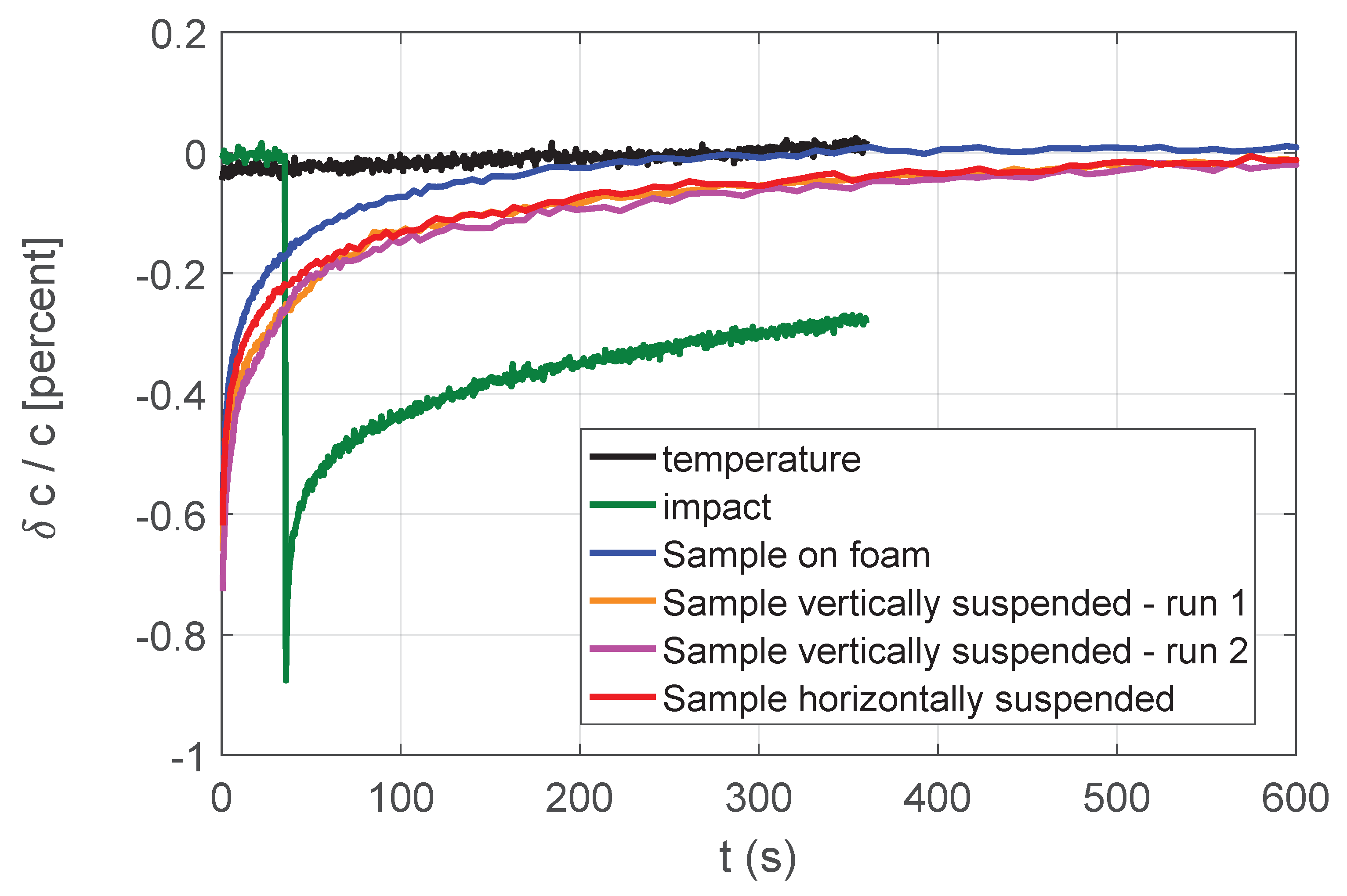
The linearity of the set-up was not an issue in the experiments conducted here, since data were acquired always at low excitation amplitudes (during both preconditioning and relaxation). Indeed, during preconditioning no nonlinear effects were shown and velocity remained constant over time. One example is given in Figure A1 as a black curve. The small drift (linear in time) is due to environmental temperature changes and it is negligible when compared with slow dynamic effects (red curve) observed in a standard experiment on the same sample.
The conditioning procedure however involved excitations at large amplitude, applied to the same transducers used for monitoring, thus a verification that the slow dynamic effects observed were not a consequence of conditioning of transducers or to variation in the boundaries was needed. To this purpose, experiments have been conducted on the same sample in different conditioning configurations.
- effects of conditioning on the transducers response were analysed modifying the conditioning process. Instead of conditioning with a sinusoidal wave (as in our approach), the sample was conditioned with an impact. A non calibrated hammer was used to produce an impact to the centre of the sample (the relaxation results are shown as a green line in Figure A1);
- effects of variations in the boundary conditions were tested by repeating the experiment in different configurations. Besides the one used in our experiments (sample suspended with vertical orientation, violet curve), we have considered the case of a sample suspended in the horizontal direction (i.e., without gravity effects, red curve) or placed horizontally on a foam layer (blue curve);
- the repeatability of the experiment was verified by repeating the experiment twice in the vertically suspended configuration (violet and yellow curves).
Figure A1.
Linearity of the experimental set up and independence of the results from the conditioning procedure. Data for the Alu-C20 sample.
Figure A1.
Linearity of the experimental set up and independence of the results from the conditioning procedure. Data for the Alu-C20 sample.

In all cases, similar relaxation curves were obtained, thus proving the slow dynamics observed was not due to boundaries or transducers conditioning. The differences in the magnitude of the effect among the various cases was expected, due to the difficulty of ensuring the same conditioning amplitude. The repeatability in the suspended cases, in which it was possible to have the same conditioning amplitude, is thus achieved also from a quantitative point of view.
References
- Guyer, R.A.; Johnson, P.A. Nonlinear mesoscopic elasticity: Evidence for a new class of materials. Phys. Today 1999, 52, 30–36. [Google Scholar] [CrossRef]
- TenCate, J.A.; Smith, E.; Guyer, R.A. Universal Slow Dynamics in Granular Solids. Phys. Rev. Lett. 2000, 85, 1020. [Google Scholar] [CrossRef] [PubMed] [Green Version]
- Scalerandi, M.; Gliozzi, A.S.; Bruno, C.L.E.; Antonaci, P. Nonequilibrium and Hysteresis in Solids: Disentangling Conditioning from Nonlinear Elasticity. Phys. Rev. B-Condens. Matter Mater. Phys. 2010, 81, 104114. [Google Scholar] [CrossRef]
- Guyer, R.A.; Cate, J.T.; Johnson, P. Hysteresis and the Dynamic Elasticity of Consolidated Granular Materials. Phys. Rev. Lett. 1999, 82, 3280. [Google Scholar] [CrossRef] [Green Version]
- Riviere, J.; Shokouhi, P.; Guyer, R.A.; Johnson, P.A. A Set of Measures for the Systematic Classification of the Nonlinear Elastic Behavior of Disparate Rocks. J. Geophys. Res. Solid Earth 2015, 120, 1587. [Google Scholar] [CrossRef]
- Feng, X.; Fehler, M.; Brown, S.; Szabo, T.L.; Burns, D. ShortPeriod Nonlinear Viscoelastic Memory of Rocks Revealed by Copropagating Longitudinal Acoustic Waves. J. Geophys. Res. Solid Earth 2018, 123, 3993. [Google Scholar] [CrossRef]
- Bittner, J.A.; Popovics, J.S. Direct Imaging of Moisture Effects during Slow Dynamic Nonlinearity. Appl. Phys. Lett. 2019, 114, 021901. [Google Scholar] [CrossRef]
- Tadavani, S.K.; Poduska, K.M.; Malcolm, A.E.; Melnikov, A. A non-linear elastic approach to study the effectof ambient humidity on sandstone. J. Appl. Phys. 2020, 128, 244902. [Google Scholar] [CrossRef]
- Chen, J.; Kim, J.-Y.; Kurtis, K.E.; Jacobs, L.J. Theoretical and Experimental Study of the Nonlinear Resonance Vibration of Cementitious Materials with an Application to Damage Characterization. J. Acoust. Soc. Am. 2011, 130, 2728. [Google Scholar] [CrossRef]
- Scalerandi, M.; Bentahar, M.; Mechri, C. Conditioning and Elastic Nonlinearity in Concrete: Separation of Damping and Phase Contributions. Constr. Build. Mater. 2018, 161, 208. [Google Scholar] [CrossRef]
- Gliozzi, A.S.; Scalerandi, M.; Anglani, G.; Antonaci, P.; Salini, L. Correlation of Elastic and Mechanical Properties of Consolidated Granular Media during Microstructure Evolution Induced by Damage and Repair. Phys. Rev. Mater. 2018, 2, 013601. [Google Scholar] [CrossRef]
- Zaitsev, V.Y.; Gusev, V.E.; Tournat, V.; Richard, P. Slow Relaxation and Aging Phenomena at the Nanoscale in Granular Materials. Phys. Rev. Lett. 2014, 112, 108302. [Google Scholar] [CrossRef] [Green Version]
- Tencate, J.A.; Shankland, T.J. Slow dynamics in the nonlinear elastic response of Berea sandstone. Geoph. Res. Lett. 1996, 23, 3019–3022. [Google Scholar] [CrossRef] [Green Version]
- Trarieux, C.; Callé, S.; Moreschi, H.; Renaud, G.; Defontaine, M. Modeling nonlinear viscoelasticity in dynamic acoustoelasticity. Appl. Phys. Lett. 2014, 105, 264103. [Google Scholar] [CrossRef]
- Cuetos, A.; Patti, A. Dynamics of Hard Colloidal Cuboids in Nematic Liquid Crystals. Phys. Rev. E 2020, 101, 52702. [Google Scholar] [CrossRef] [PubMed]
- Ilg, P. Equilibrium Magnetization and Magnetization Relaxation of Multicore Magnetic Nanoparticles. Phys. Rev. B 2017, 95, 214427. [Google Scholar] [CrossRef]
- Niss, K.; Dyre, J.C.; Hecksher, T. Long-Time Structural Relaxation of G lass-Forming Liquids: Simple or Stretched Exponential? J. Chem. Phys. 2020, 152, 041103. [Google Scholar] [CrossRef] [PubMed] [Green Version]
- Pal, P.; Ghosha, A. Broadband dielectric spectroscopy of BMPTFSI ionic liquid doped solid-state polymer electrolytes: Coupled ion transport and dielectric relaxation mechanism. J. Appl. Phys. 2020, 128, 084104. [Google Scholar] [CrossRef]
- Scalerandi, M.; Griffa, M.; Antonaci, P.; Wyrzykowski, M.; Lura, P. Nonlinear elastic response of thermally damaged consolidated granular media. J. Appl. Phys. 2013, 113, 154902. [Google Scholar] [CrossRef] [Green Version]
- Nobili, M.; Scalerandi, M. Temperature effects on the elastic properties of hysteretic elastic media: Modelling and simulations. Phys. Rev. B 2004, 69, 04105. [Google Scholar] [CrossRef]
- Ulrich, T.J. Thermally Induced Nonlinear Elasticity and Thermal Equilibrium in Berea Sandstone. Ph.D. Thesis, University of Nevada, Reno, NV, USA, 2004. [Google Scholar]
- Muir, T.G.; Cormack, J.M.; Slack, C.M.; Hamilton, M.F. Elastic softening of sandstone due to a wideband acoustic pulse. J. Acoust. Soc. Am. 2020, 147, 1006–1014. [Google Scholar] [CrossRef] [PubMed]
- Guyer, R.A.; McCall, K.R.; den Abeele, K.V. Slow elastic dynamics in a resonant bar of rock. Geoph. Res. Lett. 1998, 25, 1585–1588. [Google Scholar] [CrossRef] [Green Version]
- Scalerandi, M.; Mechri, C.; Bentahar, M.; Di Bella, A.; Gliozzi, A.S.; Tortello, M. Experimental Evidence of Correlations between Conditioning and Relaxation in Hysteretic Elastic Media. Phys. Rev. Appl. 2019, 12, 044002. [Google Scholar] [CrossRef]
- Wyrzykowski, M.; Gajewicz-Jaromin, A.M.; McDonald, P.J.; Dunstan, D.J.; Scrivener, K.L.; Lura, P. Water Redistribution-Microdiffusion in Cement Paste under Mechanical Loading Evidenced by 1H NMR. J. Phys. Chem. C 2019, 123, 16153. [Google Scholar] [CrossRef] [Green Version]
- Pecorari, C. Adhesion and Nonlinear Scattering by Rough Surfaces in Contact: Beyond the Phenomenology of the Preisach-Mayergoyz Framework. J. Acoust. Soc. Am. 2004, 116, 1938. [Google Scholar] [CrossRef]
- Guéguen, P.; Johnson, P.; Roux, P. Nonlinear Dynamics Induced in a Structure by Seismic and Environmental Loading. J. Acoust. Soc. Am. 2016, 140, 582. [Google Scholar] [CrossRef] [PubMed]
- Di Bella, A.; Scalerandi, M.; Gliozzi, A.S.; Bosia, F. Adhesion and plasticity in the dynamic response of rough surfaces in contact. Int. Solids Struct. 2021, 216, 17. [Google Scholar] [CrossRef]
- Barsoum, M.W.; Murugaiah, A.; Kalidindi, S.R.; Zhen, T. Kinking Nonlinear Elastic Solids, Nanoindentations, and Geology. Phys. Rev. Lett. 2004, 92, 255508. [Google Scholar] [CrossRef] [Green Version]
- Jin, J.; Riviere, J.; Ohara, Y.; Shokouhi, P. Dynamic Acousto-Elastic Response of Single Fatigue Cracks with Different Microstructural Features: An Experimental Investigation. J. Appl. Phys. 2018, 124, 075303. [Google Scholar] [CrossRef]
- Lott, M.; Remillieux, M.C.; Garnier, V.; Bas, P.Y.L.; Ulrich, T.J.; Payan, C. Nonlinear Elasticity in Rocks: A Comprehensive Three-Dimensional Description. Phys. Rev. Mater. 2017, 1, 1. [Google Scholar] [CrossRef] [Green Version]
- Remillieux, M.C.; Guyer, R.A.; Payan, C.; Ulrich, T.J. Decoupling Nonclassical Nonlinear Behavior of Elastic Wave Types. Phys. Rev. Lett. 2016, 116, 115501. [Google Scholar] [CrossRef] [PubMed] [Green Version]
- Johnson, P.A.; Sutin, A. Slow dynamics and anomalous nonlinear fast dynamics in diverse solids. J. Acoust. Soc. Am. 2005, 117, 124. [Google Scholar] [CrossRef] [PubMed] [Green Version]
- Mechri, C.; Scalerandi, M.; Bentahar, M. Enhancement of Harmonics Generation in Hysteretic Elastic Media Induced by Conditioning. Commun. Nonlinear Sci. Numer. Simul. 2017, 45, 117. [Google Scholar] [CrossRef]
- Setyawana, W.; Henager, C.H.; Hub, S. Nonlinear ultrasonic response of voids and Cu precipitates in body-centered cubic Fe. J. Appl. Phys. 2018, 124, 035104. [Google Scholar] [CrossRef]
- Read, T.A. The internal friction of single metal crystals. Phys. Rev. B 1940, 58, 371. [Google Scholar] [CrossRef]
- Snieder, R.; Sens-Schönfelder, C.; Wu, R. The Time Dependence of Rock Healing as a Universal Relaxation Process, a Tutorial. Geophys. J. Int. 2017, 208, 1. [Google Scholar] [CrossRef] [Green Version]
- Korobov, A.I.; Odina, N.I.; Mekhedov, D.M. Effect of slow dynamics on elastic properties of materials with residual and shear strains. Acoust. Phys. 2013, 59, 387–392. [Google Scholar] [CrossRef]
- Bentahar, M.; Aqra, H.E.; Guerjouma, R.E.; Griffa, M.; Scalerandi, M. Hysteretic elasticity in damaged concrete: Quantitative analysis of slow and fast dynamics. Phys. Rev. B 2006, 73, 014116. [Google Scholar] [CrossRef]
- Astorga, A.; Guéguen, P.; Riviere, J.; Kashima, T.; Johnson, P.A. Recovery of the resonance frequency of buildings following strong seismic deformation as a proxy for structural health. Struct. Health Monit. 2019, 18, 1966. [Google Scholar] [CrossRef]
- Mechri, C.; Scalerandi, M.; Bentahar, M. Separation of Damping and Velocity Strain Dependencies Using an Ultrasonic Monochromatic Excitation. Phys. Rev. Appl. 2019, 11, 1. [Google Scholar] [CrossRef] [Green Version]
- Di Bella, A.; Gliozzi, A.S.; Scalerandi, M.; Tortello, M. Analysis of Elastic Nonlinearity Using Continuous Waves: Validation and Applications. Appl. Sci. 2019, 9, 5332. [Google Scholar] [CrossRef] [Green Version]
- Shokouhi, P.; Riviere, J.; Guyer, R.A.; Johnson, P.A. Slow Dynamics of Consolidated Granular Systems: Multi-Scale Relaxation. Appl. Phys. Lett. 2017, 111, 251604. [Google Scholar] [CrossRef]
- Kraft, M.; Meissner, J.; Kaschta, J. Linear Viscoelastic Characterization of Polymer Melts with Long Relaxation Times. Macromolecules 1999, 32, 751. [Google Scholar] [CrossRef]
- Tong, M.; Li, L.; Wang, W.; Jiang, Y. Determining Capillary-Pressure Curve, Pore-Size Distribution, and Permeability from Induced Polarization of Shaley Sand. Geophysics 2006, 71, N33. [Google Scholar] [CrossRef]
- Vakhnenko, O.O.; Vakhnenko, V.O.; Shankland, T.J. Strain-induced kinetics of intergrain defects as the mechanism of slow dynamics in the nonlinear resonant response of humid sandstone bars. Phys. Rev. E 2004, 70, 015602. [Google Scholar] [CrossRef] [PubMed] [Green Version]
- Lieou, C.K.; Daub, E.G.; Ecke, R.E.; Johnson, P.A. Slow Dynamics and Strength Recovery in Unconsolidated Granular Earth Materials: A Mechanistic Theory. J. Geophys. Res. Solid Earth 2017, 122, 7573–7583. [Google Scholar] [CrossRef]
- Ostrovsky, L.; Lebedev, A.; Riviere, J.; Shokouhi, P.; Wu, C.; Geesey, M.A.S.; Johnson, P.A. Long-Time Relaxation Induced by Dynamic Forcing in Geomaterials. J. Geophys. Res. Solid Earth 2019, 124, 5003. [Google Scholar] [CrossRef]
- Seifi, M.; Salem, A.; Satko, D.; Shaffer, J.; Lewandowski, J.J. Defect Distribution and Microstructure Heterogeneity Effects on Fracture Resistance and Fatigue Behavior of EBM Ti-6Al-4V. Int. J. Fatigue 2017, 94, 263. [Google Scholar] [CrossRef]
- Chern, A.H.; Nandwana, P.; McDaniels, R.; Dehoff, R.R.; Liaw, P.K.; Tryon, R.; Duty, C.E. Build Orientation, Surface Roughness, and Scan Path Influence on the Microstructure, Mechanical Properties, and Flexural Fatigue Behavior of Ti-6Al-4V Fabricated by Electron Beam Melting. Mater. Sci. Eng. A 2020, 772, 138740. [Google Scholar] [CrossRef]
- Zuo, M.; Sokoluk, M.; Cao, C.; Yuan, J.; Zheng, S.; Li, X. Microstructure Control and Performance Evolution of Aluminum Alloy 7075 by Nano-Treating. Sci. Rep. 2019, 9, 10671. [Google Scholar] [CrossRef] [Green Version]
- Szemery-Kiss, S.; Torok, A. The effects of the different curing conditions and the role of added aggregate in the strength of repair mortars. Environ. Earth Sci. 2017, 76, 284. [Google Scholar] [CrossRef]
- Pugno, N.; Bosia, F.; Gliozzi, A.S.; Delsanto, P.P.; Carpinteri, A. Phenomenological Approach to Mechanical Damage Growth Analysis. Phys. Rev. E-Stat. Nonlinear Soft Matter Phys. 2008, 78, 046103. [Google Scholar] [CrossRef] [PubMed] [Green Version]
- Barzdajn, B.; Paxton, A.T.; Stewart, D.; Dunne, F.P.E. A Crystal Plasticity Assessment of Normally-Loaded Sliding Contact in Rough Surfaces and Galling. J. Mech. Phys. Solids 2018, 121, 517. [Google Scholar] [CrossRef] [Green Version]
- Uan, J.-Y.; Chang, C.-C. Gallium-induced magnesium enrichment on grain boundary and the gallium effect on degradation of tensile properties of aluminum alloys. Metall. Mater. Trans. 2006, 37, 2133. [Google Scholar] [CrossRef]
- Li, Y.; Hu, S.; Henager, C.H. Microstructure-based model of nonlinear ultrasonic response in materials with distributed defects. J. Appl. Phys. 2019, 125, 145108. [Google Scholar] [CrossRef] [Green Version]
Figure 1.
Experimental result for relaxation. (a) Linear scale; (b) Semi-logarithmic scale. Results for mortar and Al and Mg based alloys are shown to allow comparison. Data from mortar have been acquired using a protocol different than that presented here, which allows to monitor earlier times of relaxation, but, being more noisy, it could not be used to analyse relaxation in metals. For metals we obtain very small variations in the wave velocity (of the order of a few per thousands), which are comparable to resonance frequency variations induced by slow dynamics in metals observed by Johnson and Sutin [33]. Note that for longitudinal vibrations , since the resonance frequency is proportional to the wave velocity.

Figure 2.
Schematic of the experimental set up. The sample is between the transmitter (T) and receiver (R) transducers.
Figure 2.
Schematic of the experimental set up. The sample is between the transmitter (T) and receiver (R) transducers.

Figure 3.
Discrete time Fourier transform of the output signal is shown as red symbols. The resulting fit using Equation (2) is shown as a red line. The tilting corrections introduced to compensate for the transducer and source frequency responses are shown as solid black and green lines, respectively. The corrected experimental data (blue symbols) and corresponding fitting curve (blue line) are perfectly superimposed. For the sake of readability, the number of data-points was reduced by a factor of 5. Vertical dashed lines show the fitting interval for MoDANE.

Figure 4.
Reliability and accuracy of the proposed approach. Experimental resonance curves (see Figure 3 for an example) have been treated to detect the resonance frequency: Red symbols refer to the resonant frequencies detected using the MoDaNE approach (used to treat the data in our work); cyan symbols refer to peak picking of the resonance frequency using a quadratic fit of the data in a narrow region around the maximum (standard approaches). Results are equivalent but the MoDaNE approach is significantly less noisy.

Figure 5.
Multirelaxation process with decay times uniformly distributed in the log space. (a,d) Distribution of in the space for different choices of the basis range to and two different metal alloy samples (two rows). (b,c,e,f) Results of the fitting procedure for one specific choice () of the selected bases are also reported.

Figure 6.
Fitting of experimental data using a continuous Weibull distribution of relaxation times for different samples. (a) Linear scale; (b) log time scale.
Figure 6.
Fitting of experimental data using a continuous Weibull distribution of relaxation times for different samples. (a) Linear scale; (b) log time scale.

Figure 7.
Best fitting distributions for different samples. (a) One peak distributions. The first distribution for the titanium alloy is also reported for reference. (b) Two peaks distribution. The two distributions are reported separately and .
Figure 7.
Best fitting distributions for different samples. (a) One peak distributions. The first distribution for the titanium alloy is also reported for reference. (b) Two peaks distribution. The two distributions are reported separately and .

Figure 8.
Properties of the relaxation times distribution for the tested samples as a function of conditioning amplitude. (a) Area; (b) Peak position; (c) Width; (d) Centroid.
Figure 8.
Properties of the relaxation times distribution for the tested samples as a function of conditioning amplitude. (a) Area; (b) Peak position; (c) Width; (d) Centroid.

Figure 9.
Indicators quantifying the evolution of the velocity variation in time during relaxation as a function of the conditioning amplitude: (a) is the velocity variation at ; (b) is the time at which ; (c) m is the slope of the curve in the log space around , i.e., in the logarithmic recovery phase; (d) parameteric plot of m vs. .

Figure 10.
Effects of temperature variations and distributed damage in Al samples (Alu-A01 and equivalent). (a) Distribution of relaxation times for samples tested at different temperatures; (b) Distribution of relaxation times for sample with and without distributed damage; (c) Width vs. conditioning amplitude; (d) slope m vs. jump during relaxation.

Figure 11.
Effects of the presence of a closed crack. (a) Distribution of relaxation times for the intact and damaged samples. The latter is characterised by the sum of two distributions shown individually in the plot; (b) peak position vs. conditioning amplitude; (c) Width vs. conditioning amplitude.

Figure 12.
Effects of porosity on the relaxation process. (a) Distribution of relaxation times for two samples with different porosity level; (b) Peak position vs. conditioning amplitude; (c) Width vs. conditioning amplitude. Both the peak position and width are not affected by the increase of porosity. A slight increase in amplitude in correspondance to the peak of the second weibull distribution could be noticed, but data do not allow to establish with certainty whether the increase in relaxation strength is due to the increased porosity or to small differences of the two samples.

Publisher’s Note: MDPI stays neutral with regard to jurisdictional claims in published maps and institutional affiliations. |
© 2021 by the authors. Licensee MDPI, Basel, Switzerland. This article is an open access article distributed under the terms and conditions of the Creative Commons Attribution (CC BY) license (https://creativecommons.org/licenses/by/4.0/).
Share and Cite
MDPI and ACS Style
Kober, J.; Kruisova, A.; Scalerandi, M. Elastic Slow Dynamics in Polycrystalline Metal Alloys. Appl. Sci. 2021, 11, 8631. https://doi.org/10.3390/app11188631
AMA Style
Kober J, Kruisova A, Scalerandi M. Elastic Slow Dynamics in Polycrystalline Metal Alloys. Applied Sciences. 2021; 11(18):8631. https://doi.org/10.3390/app11188631
Chicago/Turabian StyleKober, Jan, Alena Kruisova, and Marco Scalerandi. 2021. "Elastic Slow Dynamics in Polycrystalline Metal Alloys" Applied Sciences 11, no. 18: 8631. https://doi.org/10.3390/app11188631
Note that from the first issue of 2016, this journal uses article numbers instead of page numbers. See further details here.