
Comparison of Two Solvers for Simulation of Single Bubble Rising Dynamics: COMSOL vs. Fluent


1
Department of Chemical Engineering, University of Chemistry and Technology Prague, Technická 3, 166 28 Prague, Czech Republic
2
Institute of Chemical Process Fundamentals of the Czech Academy of Sciences, Rozvojová 1, 165 02 Prague, Czech Republic
*
Author to whom correspondence should be addressed.
Minerals 2021, 11(5), 452; https://doi.org/10.3390/min11050452
Submission received: 25 March 2021
/
Revised: 20 April 2021
/
Accepted: 23 April 2021
/
Published: 25 April 2021
(This article belongs to the Special Issue Interactions between Bubbles and Solid Particles during the Flotation Process)
Abstract
:Multiphase flows are a part of many industrial processes, where the bubble motion influences the hydrodynamic behavior of the batch. The current trend is to use numerical solvers that can simulate the movement and mutual interactions of bubbles. The aim of this work was to study how two commercial CFD solvers, COMSOL Multiphysics and Ansys Fluent, can simulate the motion of a single rising bubble in a stagnant liquid. Simulations were performed for spherical or slightly deformed bubbles (Db = 0.6, 0.8, and 1.5 mm) rising in water or in propanol. A simple 2D axisymmetric approach was used. Calculated bubble terminal velocities and bubble shape deformations were compared to both experimental data and theoretical estimations. Solver Comsol Multiphysics was able to precisely calculate the movement of smaller and larger bubbles; due to the 2D rotational symmetry, better results were obtained for small spherical bubbles. The deformation of larger bubbles was calculated sufficiently. Solver Ansys Fluent, in the setting used, failed to simulate the motion of small bubbles due to parasitic currents but allowed for modeling of the motion of larger bubbles. However, the description of the bubble velocity and shape was worse in comparison with experimental values.
1. Introduction
Flotation is the most widely used separation process for mineral and coal processing. The key to effective particle separation is the efficient capture of hydrophobic particles by air bubbles, which is achieved via three different processes: collision, adhesion, and detachment [1,2]. The collision process involves bubbles and particles approaching each other until they collide. The probability of this subprocess is expressed as the collision efficiency, a detailed review of which can be found in the literature [3,4,5]. Here, many mathematical models are listed for estimating collision efficiency, which generally depend on the ratio of bubble to particle size and/or the ratio of bubble velocity to particle velocity.
In recent years, new studies using computational fluid dynamics (CFD) have appeared. Koh and Schwarz [6] studied collision rates in a Denver-type flotation cell and estimated the probability of collision due to the streamline effect of fine particles moving around the bubble. Schwarz et al. [7] extended their model of multiphase hydrodynamics in the Outotec flotation cell. Li et al. [8] used the CFD technique to establish a fluid mechanics model, which can directly reflect the relative motion of bubbles and particles during flotation. Wang et al. [9] developed a flotation recovery model based on first-order kinetics, where the collision efficiency was directly obtained from simulations involving a single-bubble-multiparticle aggregate system. Hassanzadeh et al. [10] published a review that summarizes the current knowledge about bubble–particle encounter including CFD simulations. They explicitly mentioned the need for a deep knowledge of fluid dynamics, which mainly concerns the description of the dynamics of the fluid flow around the moving bubble. Thus, several studies can be found that simulated two-phase flow in flotation devices. For example, Salem-Said et al. [11], using CFD, investigated two-phase (water and air) flow in a forced-air mechanically stirred Dorr–Oliver flotation machine. Farzanegan et al. [12] simulated the two-phase flow behavior in flotation columns equipped with a vertical baffle. Fayed and Ragab [13] studied the two-phase flow in a self-aerated flotation machine.
The accurate description of a bubble behavior is, thus, necessary for the proper estimation and prediction of system hydrodynamics. To this day, numerous scientific publications exist in which the authors proposed a simplified model of bubble motion in liquid. Despite their efforts, there is no universal model able to describe all bubble motion regimes in different liquids [5]. Below, we focus preferably on bubbles in flotation processes. The size of the bubbles in different flotation devices varies considerably. In industrial mechanical cells, bubbles from 0.6 to 2 mm in diameter are mostly used [10,14,15]. Column flotation uses typically bubbles with a diameter of 0.5–1.5 mm [16]. Conversely, small bubbles from 0.01 to 0.5 mm in size are recommended for the flotation of very fine particles [17,18].
Currently, commercial and noncommercial CFD tools are used to model hydrodynamic processes, including models for flotation efficiency. The best known commercial models are Ansys Fluent and COMSOL Multiphysics. This study aimed to compare both solvers for solving the hydrodynamics of a single rising bubble, the description of which is crucial for collision efficiency estimates. The manuscript explains the principles of these methods as a function of Navier–Stokes equations and provides examples of solutions to describe the behavior of bubbles.
To resolve the motion of the moving phase interface, there are two types of approaches—interface capturing and interface tracking methods [19]. The former method employs several tracking models: volume of fluid (VOF), level set (LS), phase field (PF), and constrained interpolation profile (CIP). The latter approach is used in the front-tracking method and marker-and-cell method [20].
COMSOL Multiphysics is a CFD solver based on the finite element method (FEM) [21]. FEM is one of the possible discretization methods that approximate the original partial differential equations of a solved problem. COMSOL allows the creation of the model of a whole range of multiphase phenomena from a single rising bubble to a large number of bubbles in aerated systems. COMSOL offers two built-in interface capturing models resolving the interface on a Eulerian fixed grid, namely, the level set, phase field, and one method using the arbitrary Lagrangian–Eulerian formulation (ALE), i.e., the moving mesh method. The abovementioned techniques differ in the precision of resolving the interface and in computational power requirements [21]. In this work, the level set method (LS) was used.
Another often used interface capturing method is the volume of fluid (VOF), which is implemented in the commercial CFD solver Ansys Fluent. In this case, the motion of the interface is described by the advection equation. For both phases, a quantity is introduced that describes the value of volume fraction of each phase in a control volume (computational cell) [22]. The greatest advantage of the VOF approach is mass conservation without the need for reinitialization [23].
Capabilities of different CFD solvers (commercial or in-house codes) were proven on several models of a single rising bubble or droplet. Eiswirth et al. [24] used COMSOL Multiphysics 3.3a for the study of a toluene droplet rising in a continuous aqueous phase. Šimčík et al. [22] evaluated the added mass coefficient of individual dispersed particles (bubbles) and particle clusters using the volume of fluid method in Ansys Fluent 6.1 solver. Klostermann et al. [23] used the VOF method in an open-source solver OpenFOAM to analyze the behavior of a single rising bubble with two different densities and dynamic viscosities. Experimental results of air bubbles rising in water were compared with a VOF simulation by Krishna and van Baten [25]. Yujie et al. [26] studied the dynamics of single rising bubble formation from a single orifice in Ansys Fluent 6.3. Özkan et al. [27] investigated mass transfer from an air bubble rising in a water-glycerol mixture using Ansys Fluent 12. Tripathi et al. [28] conducted a study on an initially spherical bubble rising in stagnant liquid in an open-source solver Gerris. Hysing [29] used the level set method for the case of a single rising bubble in a TP2D code and compared the results with Fluent, COMSOL, and other in-house codes. Balcázar et al. [30] created a simulation of single rising bubbles and bubble swarms using the level set method in an in-house code called TermoFluids. Analysis of the single bubble behavior proved that CFD solvers can predict the bubble motion and that they are suitable for modeling other phenomena when more bubbles are present.
All abovementioned studies dealt with larger bubbles with a diameter greater than 1 mm. The aim of this work was to describe the behavior of smaller bubbles, which are often found in multiphase apparatuses. A comparative study of different commercial CFD solvers dealing with the simulation of a single bubble rise in a stagnant liquid, validated by experimental data, has not yet been published. Therefore, the aim of this work was to compare two existing commercial CFD solvers, COMSOL Multiphysics (using LS method) and Ansys Fluent (using VOF technique), and to validate the bubble terminal velocities and shapes with experimentally determined values. The obtained data were also compared with published theoretical models working with a correlation for drag coefficient for fluid flow around a spherical particle.
2. Theoretical Description of Bubble Rise Velocity in Stagnant Liquid
Bubble rise velocity is the main quantity that determines the bubble behavior in multiphase apparatuses such as distillation and absorption columns. Many studies use simple correlations of bubble rise velocity in a stagnant liquid, where the terminal bubble velocity is derived from forces acting on the bubble in a steady state. The expression of terminal velocity Ub can be written as
where ρ is density, indices l and g denote a liquid or gaseous phase, g is the gravitational constant, Db is the bubble diameter, and CD stands for the drag coefficient. In the case of spherical bubbles, at low Reynolds number (Reb = Ub ρl Db/μl << 1), where μ is dynamic viscosity, an analogy of the flow past a rigid sphere can be used, where a symmetric flow pattern around a sphere develops. With increasing Reb, the fore-aft symmetry of the flow is distorted, and the formation of a wake becomes noticeable [31]. For larger values of Reynolds number (Reb > 50), a thin boundary layer and a narrow wake exist where the vorticity produced by the shear-free condition is confined [31,32]. Due to the no-slip condition, the bubble boundary layer separates at a larger Reb value, as compared with a rigid sphere. In the inviscid flow, the flow symmetry is recovered. In the practically interesting intermediate range of Reb, the drag coefficient cannot be found theoretically, because the problem is nonlinear and the viscous and inertia forces interplay [31]. Therefore, the approximate correlations for CD are widely used. For spherical bubbles, the expressions of Moore [32] and Mei [33] are often recommended.
The validity of the Moore drag coefficient expression was verified experimentally, and its range of validity is for spherical bubbles with Reb ≥ 50 [31]. The expression proposed by Mei is valid for all Reb; however, it does not account for bubble deformations, which occur at higher Reynolds number (Reb > 200) [33].
Furthermore, Tomiyama [34] followed other existing models and made correlations of drag coefficients for pure, slightly, and fully contaminated systems. His expressions are also applicable for nonspherical bubbles. A different approach for bubble terminal velocity was mentioned by Jamialahmadi [35]. He assumed that the motion of a large bubble is analogous to the motion of a wave in an ideal fluid.
Drag coefficients of deformed bubbles of ellipsoidal shape were also researched in many studies. The degree of deformation can be determined by the aspect ratio χ, which is the ratio between the ellipse major and minor axes [36]. Moore [32] obtained a correlation in which the aspect ratio is a function of the bubble Weber number (Web = Db ρ Ub 2/σ), where σ is the surface tension.
where is a correction factor. The drag coefficient is then calculated using the following expression:
where G(χ) and H(χ) are geometrical factors calculated by Moore [37]. Loth [38] simplified the calculation of these factors by describing them as polynomial functions of the bubble aspect ratio. Later, Rastello [39] introduced another expression for the drag coefficient of the deformed bubble. In this work, the Mei expression (Equation (3)) was modified to account for bubble nonsphericity.
The abovementioned expressions for velocity calculation (Equation (1)) and for drag coefficients (Equations (2)–(6)) were used to calculate the theoretical velocity of a single rising bubble, which was, together with the experimental data, used for validation of the simulation results.
3. Theoretical Description of Bubble Rise Velocity in Stagnant Liquid
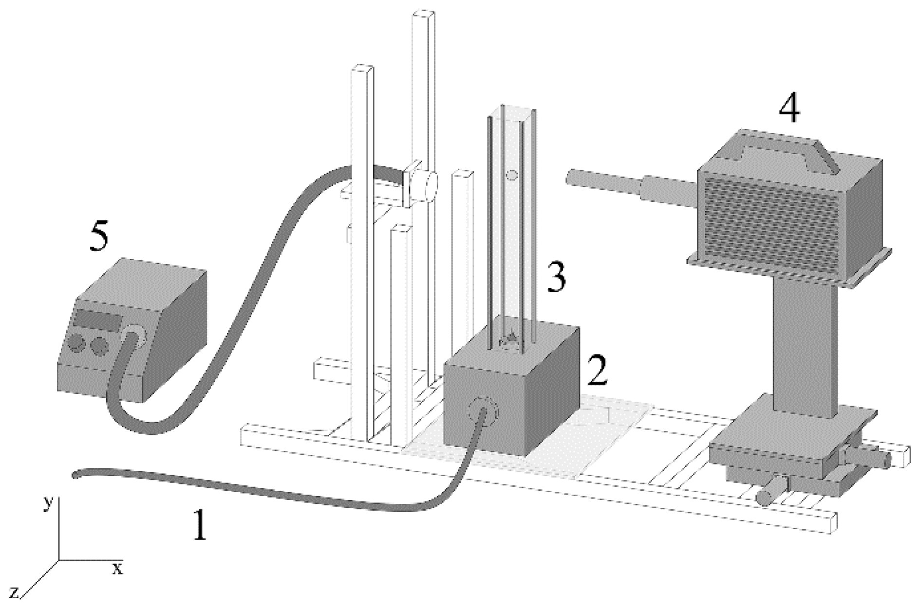
The experimental apparatus [40] consists of five main parts as seen in Figure 1. Pressurized air comes from an air compressor (1) to a filling tank underneath the bubble generator (2), which creates a bubble at the top of a thin capillary of an inner diameter 10 µm in the glass cell (3) with dimensions of 30 cm height, 8 cm width, and 6 cm depth. The size of the bubble is controlled by the gas flow rate and the growth time of the bubble. The bubble of desired size is released from the capillary by its quick pulldown. After the release, the bubble motion is captured 20 cm above the bottom of the cell, where the bubble velocity is considered steady. A Photron SA1.1 high-speed camera (4) with a 1024 × 1024 pixel resolution, 2–3 px/μm image resolution, and Navitar macro-objective lens was used to capture images of the rising bubble with a frame rate 1000 or 2000 fps. A cold light source (5) was used for area illumination.
The bubble terminal velocity was obtained from an image analysis of the captured image sequence. The NIS-Elements software was used to obtain the time dependency of tracked parameters such as the position of the bubble center of mass, bubble diameter, and aspect ratio (χ). All bubbles moved uniformly in a straight line and nonrectilinear movement was not observed, which was confirmed by the x-coordinate deviation. The distance traveled by the bubble was calculated using the x- and y-coordinates of the bubble center of two consecutive shots. The terminal rising bubble velocity was calculated by dividing the distance by the time taken to travel that distance.
where and are the distances traveled by the bubble in horizontal and vertical directions, respectively, between two consecutive images, and is a time period between these two images. The average value was determined from at least 20 consecutive bubble positions in the image frame. The experimental data for a 1.5 mm bubble rising in pure water were provided by Zedníková [41].
Theoretical Description of Bubble Rise Velocity in Stagnant Liquid
Pure water (deionized and demineralized using a water purification system “ULTRAPURE” produced by Millipore) was used at laboratory temperature for all measurements. n-Propanol with a purity of >99.5% was supplied by Penta and used as delivered without further purification. Experimental terminal bubble velocities for bubbles with diameter 0.6, 0.8, and 1.5 mm are listed in Table 1 accompanied with the physical properties (viscosity, density, and surface tension) of the liquid phase. Experimental velocities for 0.8 and 1.5 mm bubbles in propanol were not obtained due to the limitations of the experimental apparatus. Bubbles of these diameters could not be created on the capillary, as the surface tension was low, and the bubbles tore off spontaneously. In the simulations, we assumed that the air density was 1.2 kg·m−3 and the air viscosity was 1.84 × 10⁻⁵ Pa·s. A detailed description of all experimental measurements can be found in [42].
4. Computational Methods
The design of the computational domain was based on our experimental setup. The motion of a single rising bubble in a stagnant liquid and the resulting flow field are thoroughly described by the incompressible Navier–Stokes equations and continuity equations.
where ρ is the density of the fluid, u is the velocity vector, t is time, p is pressure, µ is dynamic viscosity, I is the identity matrix, and T is transposition. The term G comprises other external forces acting upon the fluid such as gravity and surface tension. However, these equations are not sufficient for a complete and mathematically accurate description of the bubble interface motion.
4.1. COMSOL Multiphysics
In COMSOL Multiphysics, the motion of the bubble was calculated using the level set method [21]. This method uses a so-called level set function φ, which is a smooth signed distance function, and its values range from 0 to 1. The interface is represented by the 0.5 contour of this function. Both phases largely differ in their density and viscosity, which causes a large discontinuity across the interface. For that reason, a smeared Heaviside function is used.
Parameter ε controls the interface thickness, and its value is set by default to half of the largest mesh element size. The transport of the level set function in its conservative form was used in order to suppress the numerical diffusion of the phase interface, and it can be expressed by the following equation:
where γ is the reinitialization parameter and is by default set to the highest value of velocity magnitude, which can occur in the domain. Similarly, the density and viscosity can be written as a function of the level set function.
where index 1 denotes the part of the domain in which the level set function is smaller than 0.5, and index 2 denotes the region where its value is greater than 0.5. These equations were solved using the built-in PARDISO solver. The pressure–velocity coupling was discretized by a P3 + P2 scheme, and the level set variable was discretized with quadratic elements. As a time stepping algorithm, the generalized alpha method was used with an automatic time step choice. Navier–Stokes equations and the level set equation were solved in a fully coupled approach. The time resolution of the results dataset was 1 ms.
4.2. Ansys Fluent COMSOL Multiphysics
In Ansys Fluent 19.1, the volume of fluid method was used. This method was introduced by Hirt and Nichols [43] in 1981. The interface movement is tracked by the value of the volume fraction in each computational cell. This value F in each cell can be easily determined.
Density and viscosity in a specific computational cell can be written using the value of the function F.
The pressure field and momentum were discretized using the PRESTO and QUICK schemes, respectively. The PISO algorithm was used for the pressure–velocity coupling, and the Geo-Reconstruct method was used for solving the interface reconstruction. This setting was adopted from the Fluent user manual [44]. The size of the time step was fixed to its value of 0.0001 s, and the results were saved every 0.01 s. The course time resolution of the results dataset was chosen to reduce the size of data.
The model used for surface tension in both CFD solvers was continuous surface force, which was introduced by Brackbill [45]. The surface tension force is added as a source term (G) in Equation (8).
where σ is the surface tension, δ is a Dirac function, and κ is the surface curvature, which is calculated as
The unit normal vector n is defined as
where C is the specific color function (level set function phi or volume fraction function F). The rise velocity of the bubble in both solvers was calculated using the following expression [46]:
where Ω2 marks the region where the value of the level set function ranges from 0 to 0.5, and u denotes the vertical component of the velocity field.
4.3. Domain Construction and Validity Check
The computational domain was constructed as a 2D axisymmetric rectangle, which corresponds to a bubble rising in a cylindrical domain, with the bubble initial position in the middle. This assumption can be used as bubbles of studied diameters stay spherical when rising and their path is rectilinear. Assumptions of the no-slip wall on both the bottom and the side of the domain, an axisymmetry condition imposed on the vertical axis, and a pressure outlet at the top of the domain were used as boundary conditions. A graphical representation of the domain is displayed in the Figure S1 (Supplementary Materials). The initial position of the spherical bubble, its diameter, and a zero-velocity field within the domain were used as initial conditions. The calculations were done on a desktop computer with an Intel i7-6700 processor and 32 GB of RAM. The duration of one simulation test case was around 10–20 h, depending on the used mesh.
The bubble velocity is influenced by the walls of the vessel if the bubble is too close to the wall [47]. To eliminate this wall effect, a study of the influence of domain width was done. The time dependency of the terminal bubble velocity for a bubble with a diameter of 0.8 mm rising in pure water was studied. The simulation was done in COMSOL, and the resulting velocities showed that the domain width of 6 mm was sufficient. A larger width of the domain (7.5 mm) did not affect the terminal bubble velocity, and only the computational time increases. For further calculations, both in COMSOL and in Fluent, domains with a width 7.5 times larger than the bubble diameter were, therefore, used.
Similar studies were conducted in both solvers to determine the mesh resolution influence on the bubble terminal velocity. Results of mesh dependency studies are outlined in Figures S2–S5 (Supplementary Materials). In COMSOL Multiphysics, this study was done for all bubble diameters. In Fluent, only the case of 1.5 mm bubble rising in propanol or water was studied, because calculations for smaller bubbles failed. A discussion concerning this problem is presented later. In COMSOL, the free triangular mesh was used, whereas, in Fluent, a mapped quadrilateral mesh was used. In both solvers, the uniform density of mesh elements across the domain was selected. For measuring this dependency, the parameter CBD (cells per bubble diameter) was used. It determines the number of computational cells covering the diameter of the bubble. In COMSOL, a sufficient value of the CBD parameter was around 15 cells. In Fluent, independent results were obtained when 100 cells covered the bubble diameter. A higher value of the CBD parameter in Fluent was chosen following the recommendations in [48].
5. Results and Discussion
The final setup of both solvers was set according to the validation studies as described above. In both COMSOL and Fluent, the width of the domain was set to 7.5 times the diameter of the bubble. Inputted initial parameters were bubble diameters (0.6, 0.8, and 1.5 mm) and the physicochemical properties of each liquid listed in Table 1. Pure water and n-propanol were used as experimental liquids. These liquids were chosen due to their significant difference in surface tension and, thus, different values of Weber number.
The simulation was terminated when a steady velocity of the bubble was reached. This velocity is called terminal, and its value was obtained as an average of the last 20 immediate velocities. To conclude, the outputs from the solvers were time-dependent values of bubble velocity, the terminal velocity, and steady-state shapes of bubbles, described by the bubble aspect ratio. Terminal velocities from CFD solvers were calculated using Equation (21), while the aspect ratios of bubbles were computed from the mirrored image sequence of the bubble rise using the image analysis software NIS-Elements.
The simulation results were compared with theoretical models. Theoretical values of the bubble terminal velocity were calculated using Equation (1) with a proper drag coefficient as described below. The bubble aspect ratios were calculated using the Moore correlation [32] given in Equation (4). The simulations were done for three different initial bubble diameters, which were chosen due to their expected shape deformations. The “small” bubble, having a diameter of 0.6 mm, was expected to stay spherical, and the terminal velocity was calculated using the Mei drag coefficient correlation (Equation (2)). The bubble with a diameter of 0.8 mm was slightly deformed; thus, the Moore expression (Equation (5)) for deformed bubbles was used to calculate the drag coefficient. To show the influence of bubble deformation on its velocity and compare the correlations, the drag coefficient was also calculated using the Mei expression (Equation (2)). In the case of a larger bubble having a diameter 1.5 mm, noticeable deformation was expected. Thus, the drag coefficient was calculated using the Moore expression (Equation (5)) and the Rastello expression (Equation (6)). Both theoretical and simulation results were compared to experimental data [41,42] if they were available.
5.1. Spherical Bubbles
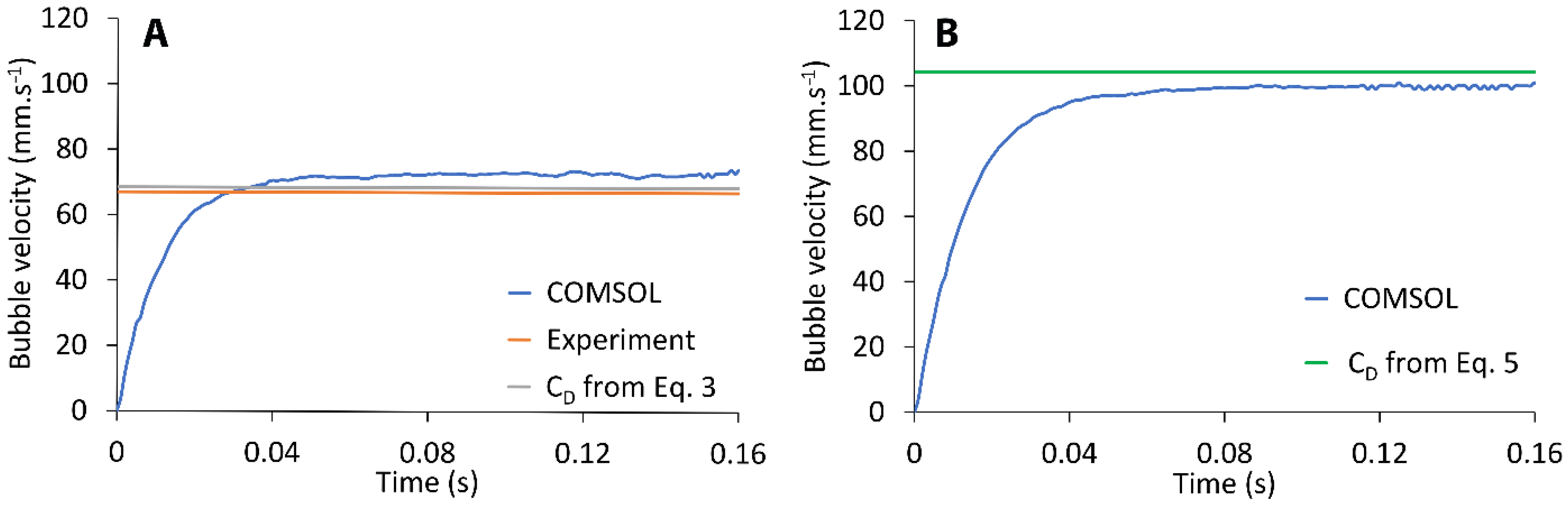
In most practical calculations, it is assumed that bubbles with a diameter below 1 mm have a fore-and-aft symmetry [49]. The more accurate estimation is given by the Weber number, which should be less than 1. In our simulations, a bubble with a diameter of 0.6 mm satisfies this condition. For a bubble with a diameter of 0.8 mm, a slight flattening can be expected. The simulation of sub-millimeter bubble motion in water or propanol converged only in COMSOL Multiphysics. In Fluent, the simulation did not converge successfully due to the parasitic currents, which appeared during the calculation. This numerical phenomenon is discussed in the last paragraph of this section. The resulting velocities from COMSOL simulations were compared to experimental data [41,42] and theoretical velocities. The results for propanol are illustrated in the Figure 2, while the results for water are shown in the Figure 3. At the same time, the bubble aspect ratios were compared. The time dependence of the velocity is considered only in the case of simulations, where the steady-state value proves the convergence of the calculation. Experimental and theoretical velocities are considered as terminal steady values.
In Figure 2, the time-dependent velocities of bubbles with diameters 0.6 and 0.8 mm rising in propanol are outlined. For the 0.6 mm bubble (Figure 2A), the experimental value of terminal velocity was 67 mm·s−1. The simulation result (73 mm·s−1) agrees with the experimental data, where the difference was 9%. The theoretical velocity calculated using Equations (1) and (3) was 68 mm·s−1. The agreement of the results is very good. The shape of the 0.6 mm bubble rising in propanol was compared to the experimental bubble aspect ratio and, concurrently, to the theoretical aspect ratio, which was estimated using the Moore correlation (Equation (4)). The deformation calculated by COMSOL (χ = 1.023) agrees with the experimental observation (χ = 1.013) and with the estimated value (χ = 1.018). Such a conclusion is also satisfactory for using the expressions for spherical bubbles when calculating the drag coefficient. Experimental data were not available for the 0.8 mm diameter bubble. Figure 2B, therefore, shows a comparison of the simulation only with the theoretical velocity. The drag coefficients calculated both using the Mei relation for spherical bubbles (Equation (3)) and Moore equation for deformed bubbles (Equation (5)) were identical; thus, only the value obtained from Moore relation is displayed in the graph. The velocity calculated using the above relationships was 104 mm·s−1. The velocity value from the simulation was 100 mm·s−1 and the difference was, thus, 4%. The aspect ratio value obtained from COMSOL (χ = 1.060) was compared only to the theoretical value (χ = 1.043), and both values are in good agreement.
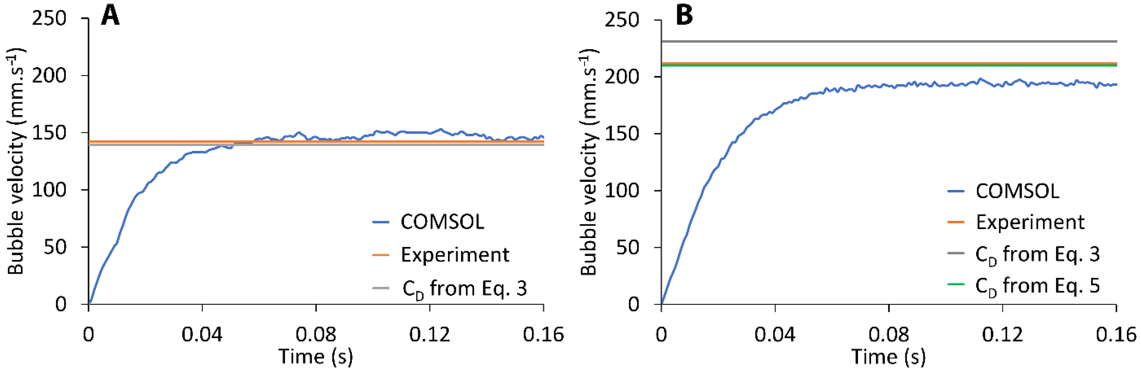
Time dependent velocities of 0.6 and 0.8 mm bubbles rising in pure water are given in Figure 3. In the case of the 0.6 mm bubble, the agreement of the COMSOL velocity (150 mm·s−1) with the experimental value (142 mm·s−1) is very good, with the COMSOL velocity being around 6% higher. Theoretical velocity of the 0.6 mm bubble was calculated using the drag coefficient for a spherical bubble (Equation (3)). The calculated value (141 mm·s−1) agrees well with experiment. The aspect ratio value of the bubble rising in water obtained from COMSOL (χ = 1.045) was slightly higher than the experimental (χ = 1.030) and theoretical (χ = 1.023) values calculated from Equation (4). Figure 3b illustrates the results for the slightly deformed bubble (Db = 0.8 mm) rising in pure water. In this case, the theoretical velocity was calculated both for spherical bubble and ellipsoidal, to discuss the importance of the bubble non-sphericity term in the drag coefficient expressions. Due to the higher surface tension of water, the Weber number is lower for the bubble in water than for the bubble in propanol; thus, greater deformations of the bubbles can be expected. The experimental bubble terminal velocity was 212 mm·s−1. Theoretical velocities were calculated for both spherical and deformed bubbles. For the spherical bubble, the drag coefficient was calculated according to Equation (3) and the related velocity was 231 mm·s−1. For the deformed bubble, the Moore expression (Equation (5)) was used. In this case, the velocity was 216 mm·s−1, which is a better match with the experiment. Using the simulation in COMSOL, a velocity of 189 mm·s−1 was obtained. A large deviation was also found for the deformation of the bubble expressed by the aspect ratio. The experimental value was χ = 1.066, whereas the COMSOL value of bubble aspect ratio was χ = 1.121. If we used this higher value of aspect ratio when calculating the theoretical velocity, we would get a value of 204 mm·s−1. It is, thus, clear that the resulting velocity is greatly influenced by the used value of the aspect ratio. We address this issue in more detail in the next section.
5.2. Moderately Deformed Bubbles
The simulation of motion of a bubble of 1.5 mm in diameter ran successfully in both CFD solvers. For bubbles of this size, significant deformation can be expected in both water and propanol. For water and this bubble diameter, Duineveld [50] stated an aspect ratio value of 1.55 and a terminal bubble velocity of about 350 mm·s−1. The theoretical bubble rising velocity calculated using the Moore expression for the drag coefficient (Equation (5)) was 390 mm·s−1, whereas that using the Rastello correlation (Equation (6)) was 346 mm·s−1. The second estimate is more accurate as it agrees with the experimentally observed velocity; thus, Rastello’s relation of the drag coefficient was used in the further calculation of the theoretical velocity. No experimental data are available for propanol. Due to the higher viscosity and lower surface tension, a lower rising bubble velocity can be expected when compared to water. Two methods were used to estimate the theoretical velocity in propanol: first, Moore’s relation of the aspect ratio (Equation (4)) together with the estimate of the drag coefficient (Equation (5)), and then Rastello’s estimation of the drag coefficient (Equation (6)). The results of both estimations were matched. The aspect ratio value was 1.043 and the theoretical velocity was 200 mm·s−1.
During the first calculation step of the simulation, the bubble was spherical; the subsequent deformation was calculated using the equations of motion and the pressure field. However, it is necessary to control the constant size, i.e., the volume of the bubble expressed by the equivalent diameter. The bubble equivalent diameter was checked by image analysis. In both solvers for bubbles rising in water and propanol, the value of equivalent diameter was almost identical to the initial diameter; thus, the value of 1.5 mm was used when determining the theoretical velocity. The resulting velocities from COMSOL simulations were compared to experimental data from [41] and theoretical velocities.
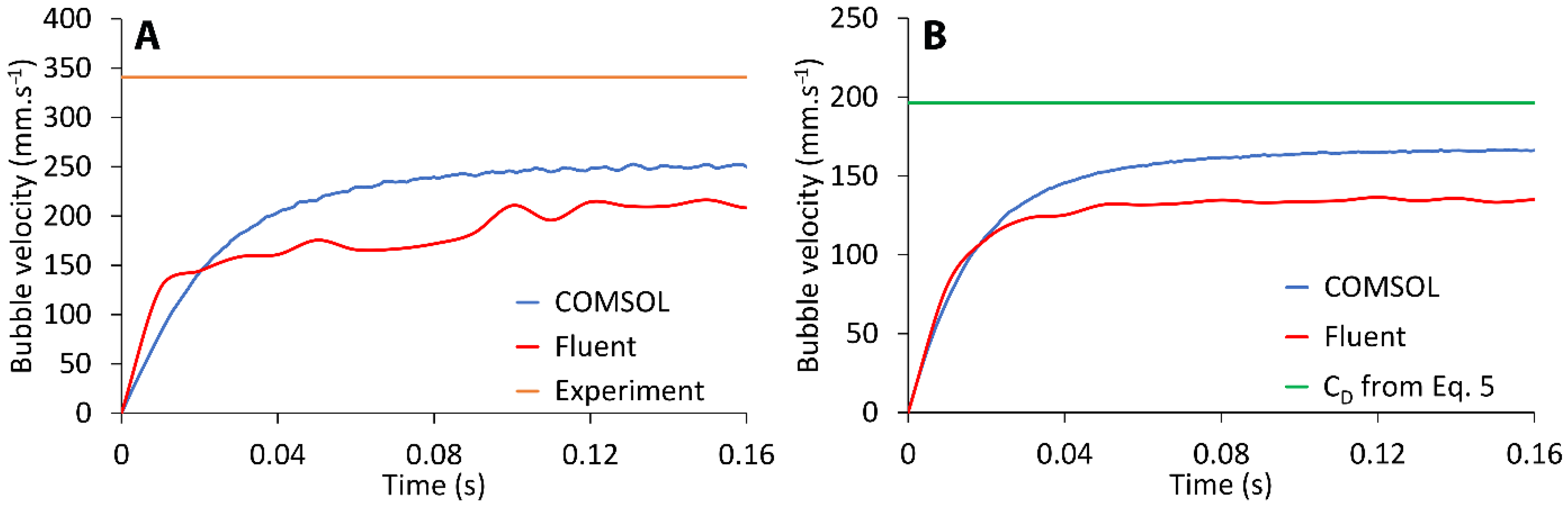
Figure 4 shows the results of the simulations done by COMSOL and Fluent together with the theoretical or experimental values. The results for water are given in Figure 4A, whereas the data for propanol are given in Figure 4B. Experimental data were only available for water [27,36]. Values of the experimental and theoretical velocities are displayed as a straight line across the time interval, as a single equilibrium value.
In the case of a bubble rising in water (Figure 4A), the velocity was compared to the experimental value. In both cases, the velocities from the solvers were quite underestimated. In COMSOL, the resulting steady-state velocity (250 mm·s−1) was around 27% lower than the experimental value of 341 mm·s−1 from [41]. The steady-state velocity obtained from Fluent (216 mm·s−1) was even lower; the difference from the experimental velocity was around 37%. The unsteady shape of the Fluent curve could have been caused by the bubble shape oscillation during the rise or by numerical instabilities. Figure 4B displays the velocities of bubbles rising in propanol obtained from both solvers compared to the theoretical velocity. In this case, the result from COMSOL (166 mm·s−1) was closer to its corresponding theoretical value, with the velocity being around 16% lower than that assumed by Equation (5) (197 mm·s−1). The velocity obtained in Fluent (133 mm·s−1) was around 32% lower.
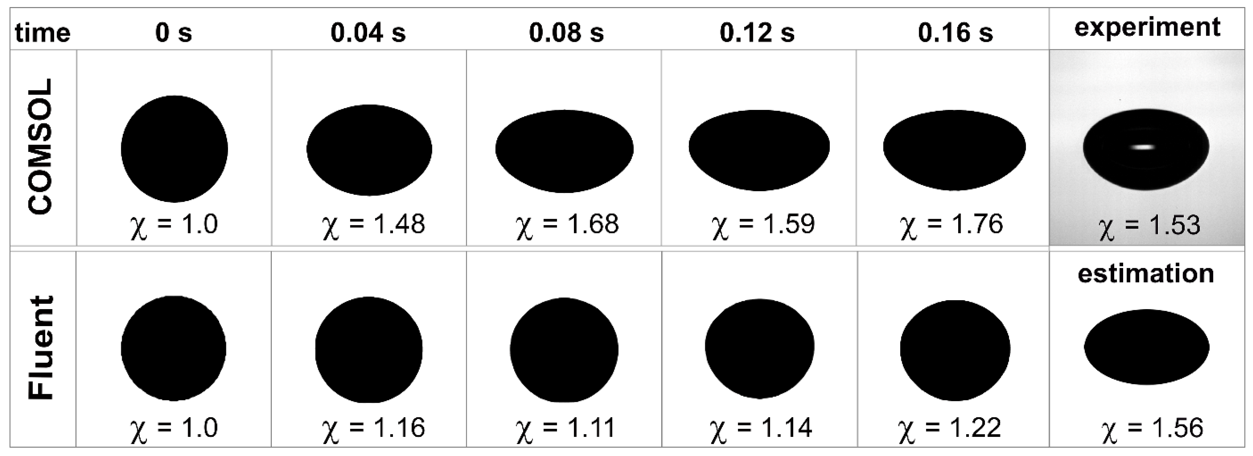
Correct description of the bubble shape is a key factor in simulating the movement of the bubble because the drag coefficient depends on the bubble aspect ratio. Therefore, the steady-state shapes of bubbles from CFD solvers were compared to theoretical and experimental results. Results for a bubble in water with Db = 1.5 mm are given in the Figure 5. The experimental aspect ratio was 1.534, whereas the estimation using Equation (4) was 1.557. The evolution of the bubble shape during the simulation is further illustrated. The simulation was terminated after 0.16 s (the equilibrium value of the aspect ratio was an average of the last 10 values), and the time step between two consecutive images was 0.04 s. During the Fluent simulation, the bubble remained almost spherical and deformed very little (χ = 1.219). As a result, the drag coefficient should be small and the bubble velocity should be high, which is not true, and the resulting velocity was lower than expected. COMSOL provided a better simulation and the bubble was sufficiently deformed during the rise. At the same time, small shape oscillations occurred. Minor oscillations were also observed during the experiments and corresponded to the limit bubble size for rectilinear motion [51]. The equilibrium aspect ratio was 1.758, which exceeded the experimental value of 1.534. A larger deformation then indicated a higher drag coefficient and a lower bubble velocity. To summarize the simulation results, an error in the aspect ratio of 15% led to an error of 27% in the velocity estimate. However, these results are very good, considering that simplistic assumptions were used, especially the assumption of 2D axisymmetry.
Obtained results from both CFD solvers and experimental measurements are clearly outlined in Table 2.
In Fluent, results were obtained only for the largest bubble diameter (1.5 mm). Simulations of both sub-millimeter bubbles failed due to the parasitic currents. Parasitic or spurious currents are nonphysical currents generated near the interface. They occur in connection with VOF or level set tracking methods and the model of surface tension forces. In this case, the model is continuum surface force (CSF). The currents arise from small deviations in the curvature of surface, which cause an error in the surface tension force and, consequently, the pressure gradient cannot balance the surface tension force. The surface tension is then balanced by velocity field component, which leads to the formation of current. Spurious currents are of great importance in surface tension-dominant regimes (large surface tension or small bubbles) [52]. These currents were also detected in COMSOL, but their magnitude was negligible compared to Fluent. Overall, the Fluent solver allowed for modeling of the movement of bubbles with a diameter over 1 mm. However, the description of the shape of the bubbles was worse in comparison with experimental values and the velocity estimate failed.
6. Conclusions
In this work, a comparison study of two commercial CFD solvers, regarding a single rising bubble problem, was carried out. Simulations of bubble movement in a stagnant liquid (pure water or 1-propanol) were performed. Simulations were done for spherical and slightly deformed bubbles, where a steady-state shape is expected. Results obtained from both CFD solvers were validated using experimental data and theoretical values. For the simulation, a simplified 2D axisymmetric model was used, which allows calculations in faster real time and can also be used for more complex calculations of more bubbles. In the next step, we will assume a similar study for a 3D model.
Modeling of bubble movement using the COMSOL Multiphysics solver (utilizing the level set method) provided very promising results. In the case of spherical bubbles, the velocity coincided with the experimental results. The values of bubble aspect ratio were higher than expected, but the relative error did not exceed 5%. In the case of deformable bubbles with a diameter over 1 mm, a description of the shape and movement was sufficient. The maximum error of aspect ratio estimation was 15%, and the velocity estimation error was up to 30%. According to these results, the COMSOL solver can be used to describe the bubble motion in a stationary liquid. The solution in 2D axisymmetry can be successfully used to simulate the shape and movement of slightly deformed bubbles. A bubble in water with a diameter of 1.5 mm can be considered as a limit value. A fully 3D model is required for larger bubbles or greater accuracy, as the bubbles tend to rise non-rectilinearly.
Results for Ansys Fluent (utilizing the volume of fluid method) were questionable. In the case of small bubbles, the calculation did not converge due to the occurrence of numerical parasitic currents. Unfortunately, even with larger bubbles, the results were worse. The deformation of the bubble was smaller than the experimental values; therefore, the agreement between the experimental and the calculated velocity was not convincing. Therefore, methods other than volume of fluid can be recommended for Fluent simulations.
Supplementary Materials
The following are available online at https://www.mdpi.com/article/10.3390/min11050452/s1: Figure S1. Scheme of the computational domain used in both CFD solvers; Figure S2. Comparison of time-dependent velocities obtained from COMSOL of a 0.6 mm bubble rising in pure water for different mesh resolutions (CBD-cells per bubble diameter); Figure S3. Comparison of time-dependent velocities obtained from COMSOL of a 0.8 mm bubble rising in pure water for different mesh resolutions (CBD-cells per bubble diameter); Figure S4. Comparison of time-dependent velocities obtained from Fluent of a 1.5 mm bubble rising in pure propanol for different mesh resolutions (CBD-cells per bubble diameter); Figure S5. Comparison of time-dependent velocities obtained from Fluent of a 1.5 mm bubble rising in pure water for different mesh resolutions (CBD-cells per bubble diameter).
Author Contributions
Conceptualization, P.B. and M.C.R.; methodology, J.C. and O.K.; software, J.C. and O.K.; validation, O.K., P.B., and M.Z.; writing—original draft preparation, J.C.; writing—review and editing, P.B., M.C.R., and M.Z.; supervision, P.B.; funding acquisition, P.B. and M.C.R. All authors have read and agreed to the published version of the manuscript.
Funding
This research was funded by the Czech Science Foundation, grant number GACR 19-09518S. This work was also supported by grants from Specific University Research, grant number A1_FCHI_2020_004 and grant number A2_FCHI_2020_017.
Conflicts of Interest
The authors declare no conflict of interest.
References
- Tao, Y.J.; Lu, M.X.; Cai, Z.; Kuang, Y.L.; Zhao, Y.M. Study of the Dynamics Characteristics for Fine Coal Flotation. J. China Univ. Min. Technol. 2003, 32, 694–697. [Google Scholar]
- Ralston, J.; Fornasiero, D.; Hayes, R. Bubble-Particle Attachment and Detachment in Flotation. Int. J. Miner. Process. 1999, 56, 133–164. [Google Scholar] [CrossRef]
- Dai, Z.; Fornasiero, D.; Ralston, J. Particle-Bubble Collision Models—A Review. Adv. Colloid Interface Sci. 2000, 85, 231–256. [Google Scholar] [CrossRef]
- Basařová, P.; Zawala, J.; Zedníková, M. Interactions between a Small Bubble and a Greater Solid Particle during the Flotation Process. Miner. Process. Extr. Metall. Rev. 2019, 40, 410–426. [Google Scholar] [CrossRef]
- Kostoglou, M.; Karapantsios, T.D.; Evgenidis, S. On a Generalized Framework for Turbulent Collision Frequency Models in Flotation: The Road from Past Inconsistencies to a Concise Algebraic Expression for Fine Particles. Adv. Colloid Interface Sci. 2020, 284. [Google Scholar] [CrossRef] [PubMed]
- Koh, P.T.L.; Schwarz, M.P. CFD Modelling of Bubble-Particle Collision Rates and Efficiencies in a Flotation Cell. Miner. Eng. 2003, 16, 1055–1059. [Google Scholar] [CrossRef]
- Schwarz, M.P.; Koh, P.T.L.; Wu, J.; Nguyen, B.; Zhu, Y. Modelling and Measurement of Multi-Phase Hydrodynamics in the Outotec Flotation Cell. Miner. Eng. 2019, 144. [Google Scholar] [CrossRef]
- Li, S.; Schwarz, M.P.; Feng, Y.; Witt, P.; Sun, C. A CFD Study of Particle–Bubble Collision Efficiency in Froth Flotation. Miner. Eng. 2019, 141. [Google Scholar] [CrossRef]
- Wang, A.; Hoque, M.M.; Moreno-Atanasio, R.; Evans, G.; Mitra, S. Development of a Flotation Recovery Model with CFD Predicted Collision Efficiency. Miner. Eng. 2020, 159. [Google Scholar] [CrossRef]
- Hassanzadeh, A.; Firouzi, M.; Albijanic, B.; Celik, M.S. A Review on Determination of Particle–Bubble Encounter Using Analytical, Experimental and Numerical Methods. Miner. Eng. 2018, 122, 296–311. [Google Scholar] [CrossRef]
- Salem-Said, A.H.; Fayed, H.; Ragab, S. Numerical Simulations of Two-Phase Flow in a Dorr-Oliver Flotation Cell Model. Minerals 2013, 3, 284–303. [Google Scholar] [CrossRef] [Green Version]
- Farzanegan, A.; Khorasanizadeh, N.; Sheikhzadeh, G.A.; Khorasanizadeh, H. Laboratory and CFD Investigations of the Two-Phase Flow Behavior in Flotation Columns Equipped with Vertical Baffle. Int. J. Miner. Process. 2017, 166, 79–88. [Google Scholar] [CrossRef]
- Fayed, H.; Ragab, S. Numerical Simulations of Two-Phase Flow in a Self-Aerated Flotation Machine and Kinetics Modeling. Minerals 2015, 5, 164–188. [Google Scholar] [CrossRef] [Green Version]
- Grau, R.A.; Laskowski, J.S.; Heiskanen, K. Effect of Frothers on Bubble Size. Int. J. Miner. Process. 2005, 76, 225–233. [Google Scholar] [CrossRef]
- Rodrigues, R.T.; Rubio, J. New Basis for Measuring the Size Distribution of Bubbles. Miner. Eng. 2003, 16, 757–765. [Google Scholar] [CrossRef]
- Dobby, G.S.; Finch, J.A. Column Flotation: A Selected Review, Part II. Miner. Eng. 1991, 4, 911–923. [Google Scholar] [CrossRef]
- Ahmed, N.; Jameson, G.J. The Effect of Bubble Size on the Rate of Flotation of Fine Particles. Int. J. Miner. Process. 1985, 14, 195–215. [Google Scholar] [CrossRef]
- Farrokhpay, S.; Filippov, L.; Fornasiero, D. Flotation of Fine Particles: A Review. Miner. Process. Extr. Metall. Rev. 2020. [Google Scholar] [CrossRef]
- Tryggvason, G.; Bunner, B.; Esmaeeli, A.; Juric, D.; Al-Rawahi, N.; Tauber, W.; Han, J.; Nas, S.; Jan, Y.-J. A Front-Tracking Method for the Computations of Multiphase Flow. J. Comput. Phys. 2001, 169, 708–759. [Google Scholar] [CrossRef] [Green Version]
- Mirjalili, S.; Jain, S.; Dodd, M. Interface-Capturing Methods for Two-Phase Flows: An Overview and Recent Developments. Cent. Turbul. Res. Annu. Res. Br. 2017, 2017, 117–135. [Google Scholar]
- COMSOL Multiphysics Reference Manual, Version 5.3; COMSOL AB: Stockholm, Sweden, 2017.
- Šimčík, M.; Růžička, M.; Drahoš, J. Computing the Added Mass of Dispersed Particles. Chem. Eng. Sci. 2008, 63, 4580–4595. [Google Scholar] [CrossRef]
- Klostermann, J.; Schaake, K.; Schwarze, R. Numerical Simulation of a Single Rising Bubble by VOF with Surface Compression. Int. J. Numer. Methods Fluids 2012. [Google Scholar] [CrossRef]
- Eiswirth, R.T.; Bart, H.J.; Atmakidis, T.; Kenig, E.Y. Experimental and Numerical Investigation of a Free Rising Droplet. Chem. Eng. Process. Process Intensif. 2011, 50, 718–727. [Google Scholar] [CrossRef]
- Krishna, R.; Van Baten, J.M. Rise Characteristics of Gas Bubbles in a 2D Rectangular Column: VOF Simulations vs. Experiments. Int. Commun. Heat Mass Transf. 1999, 26, 965–974. [Google Scholar] [CrossRef]
- Yujie, Z.; Mingyan, L.; Yonggui, X.; Can, T. Two-Dimensional Volume of Fluid Simulation Studies on Single Bubble Formation and Dynamics in Bubble Columns. Chem. Eng. Sci. 2012, 73, 55–78. [Google Scholar] [CrossRef]
- Özkan, F.; Wenka, A.; Hansjosten, E.; Pfeifer, P.; Kraushaar-Czarnetzki, B. Numerical Investigation of Interfacial Mass Transfer in Two Phase Flows Using the VOF Method. Eng. Appl. Comput. Fluid Mech. 2016, 10, 100–110. [Google Scholar] [CrossRef]
- Tripathi, M.K.; Sahu, K.C.; Govindarajan, R. Dynamics of an Initially Spherical Bubble Rising in Quiescent Liquid. Nat. Commun. 2015, 6, 1–9. [Google Scholar] [CrossRef] [Green Version]
- Hysing, S. Mixed Element FEM Level Set Method for Numerical Simulation of Immiscible Fluids. J. Comput. Phys. 2012, 231, 2449–2465. [Google Scholar] [CrossRef]
- Balcázar, N.; Lehmkuhl, O.; Jofre, L.; Oliva, A. Level-Set Simulations of Buoyancy-Driven Motion of Single and Multiple Bubbles. Int. J. Heat Fluid Flow 2015, 56, 91–107. [Google Scholar] [CrossRef] [Green Version]
- Magnaudet, J.; Eames, I. The Motion of High-Reynolds-Number Bubbles in Inhomogeneous Flows. Annu. Rev. Fluid Mech. 2000, 32, 659–708. [Google Scholar] [CrossRef]
- Moore, D.W. The Boundary Layer on a Spherical Gas Bubble. J. Fluid Mech. 1963, 16, 161. [Google Scholar] [CrossRef]
- Mei, R.; Klausner, J.F. Unsteady Force on a Spherical Bubble at Finite Reynolds Number with Small Fluctuations in the Free-stream Velocity. Phys. Fluids A Fluid Dyn. 1992, 4, 63–70. [Google Scholar] [CrossRef]
- Tomiyama, A.; Kataoka, I.; Zun, I.; Sakaguchi, T. Drag Coefficients of Single Bubbles under Normal and Micro Gravity Conditions. JSME Int. J. Ser. B Fluids Therm. Eng. 1998, 41, 472–479. [Google Scholar] [CrossRef]
- Jamialahmadi, M.; Branch, C.; Muller-Steinhagen, H. Terminal Bubble Rise Velocity in Liquids. Chem. Eng. Res. Des. 1994, 72, 119–122. [Google Scholar]
- Aoyama, S.; Hayashi, K.; Hosokawa, S.; Tomiyama, A. Shapes of Single Bubbles in Infinite Stagnant Liquids. Exp. Therm. Fluid Sci. 2016, 79, 23–30. [Google Scholar] [CrossRef]
- Moore, D.W. The Velocity of Rise of Distorted Gas Bubbles in a Liquid of Small Viscosity. J. Fluid Mech. 1965, 23, 749. [Google Scholar] [CrossRef]
- Loth, E. Quasi-Steady Shape and Drag of Deformable Bubbles and Drops. Int. J. Multiph. Flow 2008, 34, 523–546. [Google Scholar] [CrossRef]
- Rastello, M.; Marié, J.-L.; Lance, M. Drag and Lift Forces on Clean Spherical and Ellipsoidal Bubbles in a Solid-Body Rotating Flow. J. Fluid Mech. 2011, 8, 21062–21070. [Google Scholar] [CrossRef] [Green Version]
- Hubička, M.; Basařová, P.; Vejražka, J. Collision of a Small Rising Bubble with a Large Falling Particle. Int. J. Miner. Process. 2013, 121, 21–30. [Google Scholar] [CrossRef]
- Fujasová-Zedníková, M.; Vobecká, L.; Vejrazka, J. Effect of Solid Material and Surfactant Presence on Interactions of Bubbles with Horizontal Solid Surface. Can. J. Chem. Eng. 2010, 88, 473–481. [Google Scholar] [CrossRef]
- Basařová, P.; Pišlová, J.; Mills, J.; Orvalho, S. Influence of Molecular Structure of Alcohol-Water Mixtures on Bubble Behaviour and Bubble Surface Mobility. Chem. Eng. Sci. 2018, 192, 74–84. [Google Scholar] [CrossRef]
- Hirt, C.W.; Nichols, B.D. Volume of Fluid (VOF) Method for the Dynamics of Free Boundaries. J. Comput. Phys. 1981, 39, 201–225. [Google Scholar] [CrossRef]
- ANSYS Fluent Theory Guide. Available online: https://www.afs.enea.it/project/neptunius/docs/fluent/html/th/node297.htm (accessed on 13 May 2020).
- Brackbill, J.U.; Kothe, D.B.; Zemach, C. A Continuum Method for Modeling Surface Tension. J. Comput. Phys. 1992, 100, 335–354. [Google Scholar] [CrossRef]
- Hysing, S. Numerical Simulation of Immiscible Fluids with FEM Level Set Techniques. Ph.D. Thesis, Technical University of Dortmund, Dortmund, Germany, 2008. [Google Scholar]
- Krishna, R.; Urseanu, M.I.; Van Baten, J.M.; Ellenberger, J. Wall Effects on the Rise of Single Gas Bubbles in Liquids. Int. Commun. Heat Mass Transf. 1999, 26, 781–790. [Google Scholar] [CrossRef]
- Šimčík, M. Simulation of Multiphase Flow Reactors with Code Fluent. Ph.D. Thesis, University of Chemistry and Technology Prague, Prague, Czech Republic, 2008. [Google Scholar]
- Clift, R.; Grace, J.R.; Weber, M.E. Bubbles, Drops, and Particles; Academic Press, Inc.: London, UK, 1978. [Google Scholar]
- Duineveld, P.C. The Rise Velocity and Shape of Bubbles in Pure Water at High Reynolds Number. J. Fluid Mech. 1995, 292, 325–332. [Google Scholar] [CrossRef]
- Aybers, N.M.; Tapucu, A. The Motion of Gas Bubbles Rising through Stagnant Liquid. Wärme Stoffübertrag. 1969, 2, 118–128. [Google Scholar] [CrossRef]
- Harvie, D.J.E.; Davidson, M.R.; Rudman, M. An Analysis of Parasitic Current Generation in Volume of Fluid Simulations. Appl. Math. Model. 2006, 30, 1056–1066. [Google Scholar] [CrossRef]
Figure 1.
Scheme of the experimental apparatus: (1) inlet of pressurized air; (2) bubble generator; (3) glass cell with a rising bubble; (4) high-speed camera; (5) cold light source.
Figure 1.
Scheme of the experimental apparatus: (1) inlet of pressurized air; (2) bubble generator; (3) glass cell with a rising bubble; (4) high-speed camera; (5) cold light source.

Figure 2.
(A) Time-dependent velocity of a 0.6 mm bubble rising in pure propanol, compared to steady-state experimental value and theoretical computed using the Mei drag coefficient correlation (Equation (3)) for a spherical bubble (B). Time-dependent velocity of a 0.8 mm bubble rising in pure propanol, compared to steady-state theoretical value computed using Moore expression (Equation (5)) for a deformed bubble.

Figure 3.
(A) Time-dependent velocity of a 0.6 mm bubble rising in pure water, compared to steady-state experimental value and theoretical computed using the Mei drag coefficient (Equation (3)) for a spherical bubble. (B) Time-dependent velocity of a 0.8 mm bubble rising in pure water, compared to steady-state theoretical value computed using Moore expression (Equation (5)) for a slightly deformed bubble.

Figure 4.
(A) Time-dependent velocity of a 1.5 mm bubble rising in pure water, compared to a steady-state experimental value. (B) Time-dependent velocity of a 1.5 mm bubble rising in pure propanol, compared to steady-state theoretical value computed using Moore expression (Equation (5)) for deformed bubble.

Figure 5.
Comparison of the bubble shape deformation evolution in COMSOL and Fluent during the calculation time when rising in water, compared to steady-state shapes obtained from experiment and theory. Db = 1.5 mm.
Figure 5.
Comparison of the bubble shape deformation evolution in COMSOL and Fluent during the calculation time when rising in water, compared to steady-state shapes obtained from experiment and theory. Db = 1.5 mm.


Table 1.
Terminal bubble velocity and liquid density, surface tension, and dynamic viscosity at 24 °C.
Table 1.
Terminal bubble velocity and liquid density, surface tension, and dynamic viscosity at 24 °C.
| Terminal Bubble Velocity (mm·s−1) | Density (kg·m−3) | Surface Tension (mN·m−1) | Dynamic Visco-Sity (mPa·s) | |||
|---|---|---|---|---|---|---|
| Liquid | Db = 0.6 mm | Db = 0.8 mm | Db = 1.5 mm | |||
| Water | 142 | 212 | 341 | 997.1 | 72.2 | 0.89 |
| Propanol | 67 | - | - | 799.9 | 23.3 | 2.04 |
Table 2.
Summarized results from COMSOL, Fluent, and experiment for three bubble diameters (0.6, 0.8, and 1.5 mm) rising in pure water and propanol.
Table 2.
Summarized results from COMSOL, Fluent, and experiment for three bubble diameters (0.6, 0.8, and 1.5 mm) rising in pure water and propanol.
| Water | Propanol | ||||||
|---|---|---|---|---|---|---|---|
| Bubble Diameter (mm) | 0.6 | 0.8 | 1.5 | 0.6 | 0.8 | 1.5 | |
| Bubble Velocities (mm·s−1) | |||||||
| Experiment | 142 | 212 | 341 | 67 | - | - | |
| COMSOL | 150 | 189 | 250 | 73 | 100 | 166 | |
| Fluent | - | - | 216 | - | - | 133 | |
Publisher’s Note: MDPI stays neutral with regard to jurisdictional claims in published maps and institutional affiliations. |
© 2021 by the authors. Licensee MDPI, Basel, Switzerland. This article is an open access article distributed under the terms and conditions of the Creative Commons Attribution (CC BY) license (https://creativecommons.org/licenses/by/4.0/).
Share and Cite
MDPI and ACS Style
Crha, J.; Basařová, P.; Ruzicka, M.C.; Kašpar, O.; Zednikova, M. Comparison of Two Solvers for Simulation of Single Bubble Rising Dynamics: COMSOL vs. Fluent. Minerals 2021, 11, 452. https://doi.org/10.3390/min11050452
AMA Style
Crha J, Basařová P, Ruzicka MC, Kašpar O, Zednikova M. Comparison of Two Solvers for Simulation of Single Bubble Rising Dynamics: COMSOL vs. Fluent. Minerals. 2021; 11(5):452. https://doi.org/10.3390/min11050452
Chicago/Turabian StyleCrha, Jakub, Pavlína Basařová, Marek C. Ruzicka, Ondřej Kašpar, and Maria Zednikova. 2021. "Comparison of Two Solvers for Simulation of Single Bubble Rising Dynamics: COMSOL vs. Fluent" Minerals 11, no. 5: 452. https://doi.org/10.3390/min11050452
Note that from the first issue of 2016, this journal uses article numbers instead of page numbers. See further details here.