
Temporal Dynamics of CO2 Fluxes over a Non-Irrigated Vineyard
by
 , , , ,
Aysan Badraghi
1,2,*,
Beáta Novotná
1,
Jan Frouz
2,3,
Koloman Krištof
4,
Martin Trakovický
5,
Martin Juriga
6,
Branislav Chvila
7 and
Leonardo Montagnani
8,9
1
Institute of Landscape Engineering, Slovak University of Agriculture in Nitra, Tr. A. Hlinku 2, 949 76 Nitra, Slovakia
2
Institute for Environmental Studies, Charles University, Fac. Sci. Benatska 2, 128 00 Prague 2, Czech Republic
3
Institute of Soil Biology and Biogeochemistry, Biology Centre CAS, Na Sadkach 7, 370 05 Ceske Budejovice, Czech Republic
4
Institute of Agricultural Engineering, Transport and Bioenergetics, Slovak University of Agriculture in Nitra, Tr. A. Hlinku 2, 949 76 Nitra, Slovakia
5
TRAKO, s.r.o. Pod lesom 11, 949 01 Nitra, Slovakia
6
Institute of Agronomic Sciences, Slovak University of Agriculture in Nitra, Tr. A. Hlinku 2, 949 76 Nitra, Slovakia
7
Meteorological and Climatological Monitoring, Slovak Hydrometeorological Institute, Jeséniova 17, 833 15 Bratislava, Slovakia
8
Faculty of Science and Technology, Free University of Bozen-Bolzano, Piazza Università 1, 39100 Bolzano, Italy
9
Forest Services, Autonomous Province of Bolzano, Via Brennero 6, 39100 Bolzano, Italy
*
Author to whom correspondence should be addressed.
Land 2023, 12(10), 1925; https://doi.org/10.3390/land12101925
Submission received: 30 August 2023
/
Revised: 12 October 2023
/
Accepted: 14 October 2023
/
Published: 16 October 2023
Abstract
:Some knowledge gaps still remain regarding carbon sequestration in non-irrigated agroecosystems, where plants may experience drought stress during summertime. Therefore, by the combination of the eddy covariance (EC) and soil chamber techniques, we determined the role of a non-irrigated grassed vineyard in carbon sequestration in the Slovak Republic. Based on the EC data, the cumulative net uptake of CO2 (NEE) for the whole growing season was weak and was ca. −97 (g C m−2). This value resulted from −796 (g C m−2) carbon uptake from the atmosphere through photosynthesis (GEE) and 699 (g C m−2) carbon released to the atmosphere through respiration (Reco). Carbon emissions through Reco were considerable and accounted for ca. 88% of GEE, which points out the importance of Reco for managing non-irrigated agroecosystems. Data from the soil chamber indicated that ca. 302 g C m−2 was released by the vineyard through soil respiration (Rsoil) over a growing season, which was constantly lower than Reco and accounted for ca. 44 ± 18% of Reco. This finding implies that the vineyard soil was not a main source of carbon emissions. Rsoil was mainly driven by temperature (exponentially ca. 69–85%). Meanwhile, vapour pressure deficit (VPD) and temperature appeared to be the most important limiting factors for GEE, NEE, and Reco, particularly when they exceeded a certain threshold (e.g., temperature > 17 °C, and VPD > 10 hPa).
1. Introduction
Anthropogenic emissions of carbon dioxide (CO2) are on the rise due to human activity and have increased the atmospheric CO2 by ca. 40% compared to the pre-industrialization period [1,2]. The increase in CO2 has a direct impact on climate change and global warming by changing the radiation force of the atmosphere [3]. Plants and soil can absorb a substantial part of anthropogenic CO2 emissions [4]. Therefore, they have the potential to be important carbon sinks, and with proper management, an agroecosystem can sink about 690 and release about 275 g C m−2 yr−1 to the atmosphere [5,6]. However, carbon dynamics in agroecosystems can also be influenced by harvested yield, soil and crop type, and climate [5,7,8].
Perennial crops, in addition to food production, have the potential to sequester and store carbon on a long-term basis, which can help mitigate the anthropogenic production of CO2 [9,10,11,12]. Viticulture, with an area of ca. 7.3 million hectares, is still one of the most widespread agricultural production systems around the world [13]. Therefore, its potential for carbon capture and storage has gained attention, and researchers have increasingly focused on carbon sequestration in vineyards across the world, particularly in Europe, where 40% of the vineyard area is located [14,15,16,17,18,19,20]. On the other hand, undisturbed soil in perennial tree crops, apart from the reduction of carbon emissions [21], can be a good example for assessing carbon emissions from soil in the agroecosystem where the impact of tillage and heavy machines passing on soil respiration (Rsoil) is minimized [22,23,24,25]. However, other factors such as temperature, moisture, soil properties, nitrogen fertilizer, and microbial activities can also affect Rsoil as a fraction of ecosystem respiration [26,27,28]. In general, Rsoil is the largest component of Reco, as evidenced by previous studies [29,30,31], even though some investigations have reported a lower value of Reco in comparison to Rsoil [32,33]. Nevertheless, the most recent estimations from an Italian vineyard suggest that Rsoil accounts for 83% of Reco [10]. In this context, soil can play an important role as a major carbon reservoir in the global carbon budget, but it is inadequately understood, particularly in the agroecosystem. Therefore, quantifying the amount of Rsoil in parallel with Reco can provide detailed information concerning the main source of the released CO2 efflux to the atmosphere in the perennial cropland.
Presently, eddy covariance (EC) is the most widely used technique for monitoring the net ecosystem exchange of CO2 (NEE), which results from two larger fluxes of opposite signs: CO2 uptake by photosynthesis (GEE) and CO2 release by Reco [34,35,36,37,38]. Therefore, EC has recently been employed to quantify CO2 fluxes in vineyards [39,40], particularly in Italy, where vineyards have demonstrated a moderate carbon sink capacity [10,41,42]. However, an irrigated vineyard within an arid region of China acted as a strong carbon sink [39]. In the Slovak Republic, agricultural land covers 46.4% of the total area, and about 5% of agricultural land is given over to perennial tree crops [43]. Although half of the country is covered by agroecosystems, limited studies properly consider the carbon potential of agroecosystems. Furthermore, most studies that have investigated carbon fluxes in vineyards were supplied by irrigation systems. In particular, in areas with hot dry summers where plants may experience drought stress during summertime, carbon fluxes can be affected as a consequence. Therefore, to improve understanding of CO2 flux patterns in woody crops (with ongoing climate change), this study was conducted in non-irrigated agroecosystems with mild winters and relatively hot and dry summers by employing EC and chamber-based measurements. Considering the potential for drought stress in this area during summer, our specific hypothesis is that a non-irrigated vineyard cannot act as a strong sink of carbon.
In fact, this study aims to determine (i) whether non-irrigated grassed vineyards act as a carbon sequester or emitter; (ii) since soil remains undisturbed for decades in many perennial crops, whether aboveground respiration is the main fraction of Reco, i.e., is Reco consistently higher than Rsoil from daily to seasonal scales because of undisturbed soil; and (iii) how CO2 fluxes (NEE, GEE, Reco, and Rsoil) respond to environmental variables.
2. Materials and Methods
2.1. Site Description
The study was performed in a 47-year-old vineyard in Nevidzany village, Zlaté Moravce municipality (Tekov region) which is located in the western part of the Slovak Republic (48°16′22″ N and 18°22′35″ E; 220 m a.s.l). The vineyard under experimentation covered an area of 20 hectares on homogenous terrain with a 5% slope. The planting density was ca. 4000 vines/ha−1 with a 3 × 0.8 m distance. The vine varieties were Riesling and Cabernet Sauvignon, grafted on Kober 5BB rootstock. The training system was cordon.
The vineyard soil was covered by grasses and classified as brown soil type, subtype: Pseudogley brown soil, with signs of anthropic activity in the humus horizon. The original parent material that formed the soil-forming substrate for the emerging soil was loess, and in some parts of the area of interest, loess and polygenetic clays (soil survey taken by the Department of Pedology and Geology, Institute of Agronomic Sciences, Faculty of Agrobiology and Food Resources, Slovak Agricultural University in Nitra, 2022). The climate, in general, is dry and warm with mild winters, and the area receives an average annual precipitation of 662 mm; the mean annual temperature is 9 °C [44].
During the measurement period, a combination of B. megaterium and micro-dosed NPK fertilizer was applied once on the leaves, and pesticide spraying was used for pest-control purposes three times. Dormant pruning was performed in March, and prunings were chopped (into smaller pieces) or mulched in the vineyard alleys and used as a source of nutrients for the covered grass, soil, and grapevines. In addition, the cover grass was mowed three times in April, July, and November, and grass clippings were also used as soil surface mulch in the vineyard alleys. The grape production was 5.5 tons per hectare for the year 2022.
To provide an overview of the soil’s chemical and physical characteristics, we quantified parameters such as soil organic carbon and nitrogen, soil pH, bulk density, soil porosity, and soil water retention. The results of these measurements are presented in detail in Table 1. Additionally, our assessment of soil texture demonstrated that ca. 68% of the soil proportion was clay-silt (0.001–0.05 mm; Table A1).
2.2. Instrumentation and Measurements
2.2.1. Eddy Covariance
An eddy covariance tower was mounted at 3.0 m height above the soil surface to quantify the CO2 fluxes’ exchange between the vineyard ecosystem and atmosphere (NEE). The measurement was performed for a growing season (April–September 2022). The EC consisted of an enclosed-path infrared gas analyzer (IRGA analyzer Li-7200 from LI-COR Biosciences, Lincoln, NE, USA) to monitor GHG fluxes continuously, a 3-dimensional sonic anemometer (CSAT3, Campbell Scientific Inc., Logan, UT) to collect wind velocities and sonic temperature, and a datalogger to store 10 Hz raw data (CR3000, Campbell Scientific Inc., Logan, UT, USA). To calculate the 30 min average fluxes of CO2, the high-frequency binary data (TOB1) was converted into the ASCII format with a 30 min timestep, using LoggerNet (Campbell Scientific Inc., Logan, UT, USA). Then, its output (ASCII files) was processed by the Eddypro software packages developed by the Li-Cor Company (LI-COR, Lincoin, NE, USA). After calculating the 30 min average fluxes (of CO2, LE and H), the data were quality-checked [45], de-spiked [46,47], and filtered according to friction velocity [48,49], and double coordinate rotation was used to tilt correction [50]. The u⁎ threshold was detected using the R package REddyProc [46]. Gap filling was carried out using the techniques outlined by Falge et al. [51] and Reichstein et al. [49], and the uncertainty of the gap-filled half-hourly data was estimated. Partitioning of NEE into GEE and Reco was also done by REddyProc [46], based on the nighttime method [49]. Then, biological flux parameters (NEE, GPP, Reco) were aggregated into daily and monthly values, and those for the whole growing season [46,52]. All steps of post-processing were done by the REddyProc package in R [46].
2.2.2. Soil Chamber
Soil respiration (Rsoil) measurements were conducted in parallel with EC continuously (1 h intervals) using an Automated Soil CO2 Exchange System (ACE, ADC BioScientific Ltd., Hoddesdon, UK). The measurements were taken within the footprint of the EC tower in the vine rows, as it was not possible to measure in the alleys due to machine passage. Measurements were taken using the measured CO2 concentration by soil chamber; then, soil CO2 effluxes were measured as follows [53], (Equation (1)):
where Rsoil is soil respiration (µmol m−2 s−1); us is the molar flow of air per square meter of soil (mol m−2 s−1); and ∆c is the difference in CO2 concentration through the soil chamber.
Rsoil = us × (−∆c)
The nonlinear least squares (NLS) regression is the most widely used method for the gap-filling of soil CO2 efflux [54]. Therefore, to fill the gaps in soil CO2 efflux, we applied (i) the Q10 [55] (Equation (2)), and (ii) the logistic model [56] (Equation (3)), by using the nls package in R software [57]. The best-fitted models were used to fill the gaps in Rsoil (based on Akaike’s Information Criterion (AIC), R-squared (R2), Mean Absolute Error (MAE), and Root Mean Squared Error (RMSE)). The Q10 model was also used to estimate the Q10 value.
where Rsoil is the soil respiration; Rref is the fitted Rsoil at the reference temperature of 10 °C (Tref); Q10 is the temperature sensitivity of Rsoil, defined as the factor by which Rsoil increases with a 10 °C temperature increase; and T is soil temperature.
where Rsoil is soil respiration; a is the maximum value of Rsoil; b determines the elongation of the Rsoil curve along the x-axis; k is the logistic growth rate or steepness of the Rsoil curve along the x-axis; and T is soil temperature.
After computing Reco and Rsoil, the aboveground respiration (RAG) was calculated as below [Equation (4)]:
RAG = Reco − Rsoil
2.2.3. Soil Properties and Meteorological Variables
To analyze soil properties, we collected 15 soil samples at a depth of 10 cm. Soil samples were oven-dried (at 110 ± 5 °C), weighed, and sieved (2 mm mesh size) in the laboratory. Soil bulk density was determined by dividing the weight of dried soil by the sample volume [58]. The pipette method was used for soil texture determination [59]. Soil porosity and soil water retention were determined as described by Spasić et al. [60]. The determination of soil nitrogen (N) was done by the Kjeldahl Method [61], and soil organic carbon (C) was estimated by the Walkley and Black Method [62]. Soil pH was measured by a pH meter with soil having a deionized water ratio of 1:2.5 (m:v; ino Lab pH 730, Carl Stuart Limited, Tallaght Business Park, Dublin 24, Ireland).
Climate variables including soil temperature (at 10 cm depth; PT100/8, EMS, Czech Republic), air temperature, relative humidity (at a height of 2 m above ground level; HMP155C probe, Vaisala Corporation, Helsinki, Finland), and the global radiation (Rg; CMP 6 pyranometer, AZO, Czech Republic) were collected in 30 min intervals (April–September 2022). Daily sum precipitation (MR3H-01s, METEOSERVIS, Czech Republic) was collected from the nearest meteorological station (meteorological station in Mochovce; 2 km). Vapour pressure deficit (VPD) was estimated by REddyProc from air temperature and RH [46]. The estimation of the energy budget closure was not possible due to the absence of sensors for net radiation and soil heat flux.
2.3. Data Analysis
All statistical comparisons were performed by the ANOVA (normally distributed data; Tukey test, p < 0.05) or the Kruskal–Wallis test (non-normally distributed data; Dunn test, p < 0.05) after assessing the normality of the data and homogeneity of the variance [63,64]. All statistical analyses were performed by R version 4.1.12 [65]. The regression analyses were used to examine the response of NEE, GEE, Reco, and Rsoil to the environmental factors.
3. Results
3.1. Meteorological Variables
Seasonal patterns of daily averages of the main environmental variables over a growing season (April–September) are presented in Figure 1. Overall, the air and soil temperature (°C), vapour pressure deficit (VPD, hPa), global radiation (Rg; MJ m−2 d−1), and latent (LE; MJ m−2 d−1) and sensible heat flux (H; MJ m−2 d−1) values gradually increased as the growing season progressed; once they reached their peak in June/July/August, they started to decline again and reached their lowest value at the end of the growing season. At the same time, an opposite pattern was detected for relative air humidity (RH%) (Figure 1).
During our measurement period, the warmest months were June, July, and August, and April was the coldest (Figure 2a,b; p < 0.001). Further, we found that the soil temperature at a depth of 10 cm exceeds the atmospheric temperature (Figure 1a). The highest value of Rg was recorded for June and the lowest value for September (Figure 2c). LE in May and June was significantly higher than in other months, while June and July were the months with the highest value of H (Figure 2d,e). The driest period of our measurement period was between April–July, and the amount of precipitation during April–July was significantly lower than in August and September; the majority of the precipitation fell at the end of the growing season (Figure 2f). RH showed the opposite pattern to VPD; RH reached its lowest value in July when the highest value of VPD was recorded. On the other hand, September was the month with the lowest value of VPD and the highest value of RH (Figure 2g,h).
3.2. Dynamics of CO2 Fluxes
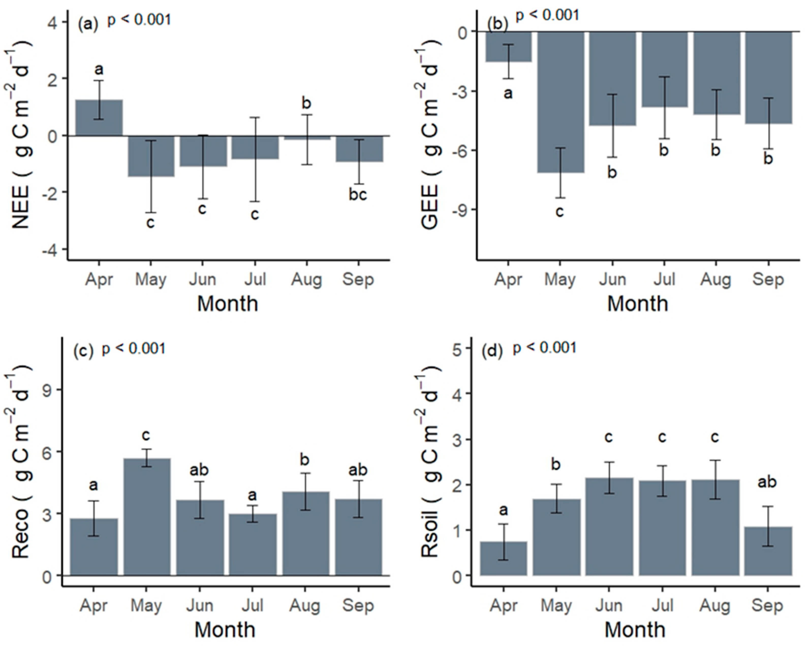
In total, NEE or the net uptake of CO2 for the whole growing season was ca. −97 g C m−2. Our case study ecosystem uptake was ca. −799 g C m−2 from the atmosphere through photosynthesis (by convention, CO2 uptake from the atmosphere has a negative sign; therefore, NEE and GEE < 0). On the other hand, it released ca 699 g C m−2 to the atmosphere through respiration (Reco), for the whole growing season. Diurnal averaged NEE fluxes were −0.53 ± 1.03 g C m−2 d−1, which varied between −4.06 and 3.36 g C m−2 d−1. Its value was almost negative during May–September; in contrast, it acted as a source of CO2 during April, which is indicated by the positive values. The mean daily value of GEE was −4.35 ± 1.30 g C m−2 d−1, and the mean daily value of Reco was 3.82 ± 0.72 g C m−2 d−1 (Figure 3).
The highest value of the net CO2 uptake was during May (−1.44 ± 1.27 g C m−2 d−1) and was significantly higher than in April and August. The lowest value was recorded for April (1.27 ± 0.69 g C m−2 d−1; Figure 3a) which was significantly lower than other months. In the meantime, the highest amounts of gross productivity and ecosystem respiration were also recorded for May and the lowest value for April (Figure 3b).
3.3. Diurnal and Seasonal Variability in Rsoil
The cumulative carbon loss by the vineyard soil was ca. 302 g C m−2 for a growing season, and the mean diurnal cumulated Rsoil was 1.65 ± 0.37 g C m−2 d−1. The lowest value of Rsoil was observed in April (0.75 ± 0.39 g C m−2 d−1) and the highest value in June (2.15 ± 0.35 g C m−2 d−1). The Rsoil values in June, July, and August were significantly greater than in April, May, and September (Figure 3d). Overall, Rsoil exponentially followed the trend of soil temperature, and 69–85% of the variation in Rsoil was explained by temperature (Table A2).
3.4. Comparing Reco and Rsoil
Overall, Rsoil accounted for ca. 44 ± 18% of Reco for the whole measurement period and was consistently lower than Reco (Figure 4b). The proportion of Rsoil to Reco varied between months (27% to 70%; Table 2): Rsoil in Jul accounted for the highest fraction of Reco (70%; Table 2), while in April, Rsoil accounted for 27% of Reco. Aboveground respiration (RAG) accounted for ca. 56 ± 27% of Reco. May (4.01 ± 0.11) reached the highest value of RAG, and the lowest value of RAG was recorded for July (0.90± 0.06; Table 2).
Further, our result indicated that the temperature sensitivity (Q10) of both Reco and Rsoil is similar during the cooler months (April and September), but during the warmer months (May, June, July, and August), the Q10 value from Rsoil is almost twice that of Reco. In contrast, computed Rref from Reco is notably higher than Rsoil for all six months (Table 2).
3.5. Response of CO2 Fluxes to Major Environmental Variables
All flux parameter (NEE, GEE, Reco, Rsoil) responses were almost significant to temperature, VPD, and Rg. On the contrary, no significant correlations were detected between precipitation and CO2 fluxes (Figure 5). The net and gross uptake of CO2, and Reco tended to increase with the increasing temperature and VPD. They reached their peak at specific values of temperature (ca. 17 °C) and VPD values (10 hPa). Then, their value started to decline with further increases in temperature and VPD. Based on the R-square (R2) values, Rg (R2 = 0.32) and VPD (R2 = 0.29) were identified as the most important driving factors for NEE. Meanwhile, temperature and VPD were detected as the main driving factors for Rsoil, Reco, and GEE (Figure 5).
4. Discussion
4.1. Variability in NEE, GEE, and Reco
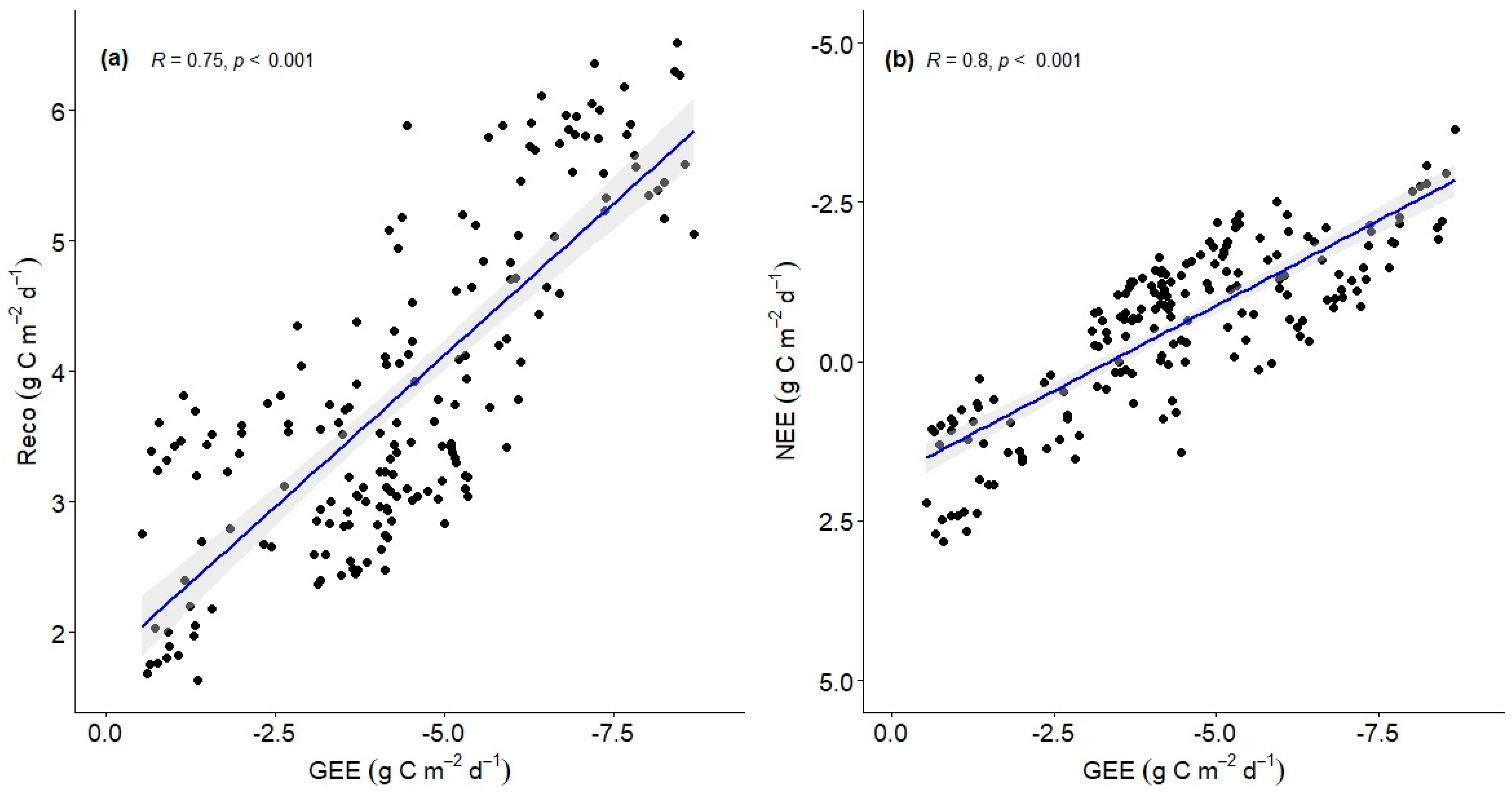
The reported amounts of annual net carbon accumulation in vineyards ranged between −69 to −961 g c m−2 yr−1 [10,19,23,39,40,42,66], and some of them were considerably higher than our finding (−97 g C m−2). In fact, the higher values of NEE in these research findings resulted from the lower values of Reco. For instance, in the arid area of China where a vineyard reached the highest value of NEE [−961 g c m−2 yr−1; 39], the annual GEE was ca. −1274 g c m−2 yr−1, which is not considerably more than our finding (−796 g C m−2 for a growing season). But they could record the highest amount of NEE due to a lower value of Reco (286 g c m−2 yr−1), which was much smaller than our finding (699 g C m−2 for a growing season). Therefore, despite a higher amount of GEE, the role of our vineyard in carbon sequestration was weak [41], because ca. 88% of carbon uptake was released again into the atmosphere through respiration. However, this value was ca. 90% of GEE in an irrigated vineyard in Italy [10], while it accounted for just 22% of GEE in China and made it a strong carbon sink [39]. This finding suggests the importance of Reco for agroecosystem management for carbon sequestration.
In perennial systems, cover crop mowing can raise the amount of greenhouse gas (GHG) emissions even up to 10–20 times after subsequent irrigation or precipitation [67,68]. Therefore, a possible explanation for the higher amount of Reco could be frequent mowing and surface mulching by grass clippings and pruned branches. The retention of grass clippings on the soil surface during April, July, and November, and returning pruned branches as the surface mulch in March, probably increased carbon emission (Reco) in our study site due to rapid decomposition [19]. A study from the USA also found a significant effect of mowing on Rsoil, particularly after rainfall [21]. However, in our study, mulching may not affect the Rsoil, because Rsoil measurements were performed on the vine rows, and grass clippings were left on the tractor row (alleys) surface. More work is needed to verify the mulching effect on Rsoil, and consequently, Reco.
4.2. CO2 Flux Response to Environmental Variables
May was the month that reached the highest value of NEE (negative value), GEE, and Reco (Figure 3). An increase in NEE is expected with increasing GEE; on the other hand, with an increase in GEE, larger crop biomass is also expected, which provides more respiring tissues [69]. Therefore, an increase in GEE consequently increased NEE and Reco. However, in contrast to our finding, the highest value of NEE in the irrigated vineyards was reported for the mid-growth stage [19,39]. A study in a forest area attributed the lower value of NEE at the mid-growth stage to the high Rsoil [70]; this might also be a reason for our case study, as we found the highest amount of Rsoil for the mid-growth stage (Figure 3d). Besides the high values of Rsoil, the water limitation in combination with heat stress can be the most important reason that June, July, and August acted as weak sinks of carbon in our case study [49,71]. As Figure 5 has shown, VPD and temperature can be limiting factors when they exceed a certain threshold, e.g., once the temperature is higher than ca. 17 °C and VPD is higher than ca. 10 hPa (Figure 5) [72]. Therefore, a higher amount of NEE and GEE in May could be induced by the coupling of warmer weather (16.5 ± 1.5 °C; Figure 2a) with a lower value of VPD/water stress (7.3 ± 2.2 hPa); [28,73,74,75]. Meanwhile, based on our result, 75% of Reco is explained by GEE (Figure A1); [29,76]. In this context, the highest amount of Reco in May is also reasonable [74]. May was the month with the lowest rainfall (Figure 2f); nevertheless, the highest values of NEE, GEE, and Reco were found for this month. Probably, the lower value of VPD maintains higher stomatal conductance, thereby potentially triggering an increase in the photosynthesis rate and subsequently leading to higher NEE and Reco values [73,77]. Alternatively, a higher amount of Rg could be another influencing factor, considering the significant correlations observed between NEE and GEE with Rg (Figure 5); [23]. Conversely, the high VPD associated with high temperatures and low rainfall during the summer months might suppress the photosynthesis rate and decrease productivity in our non-irrigated vineyard, particularly in July (Figure 2a,f,h and Figure 3). This observation implies the importance of water availability in carbon sequestration [69,78,79,80] and aligns with the findings of Marras et al. [19], who suggested that a vineyard can reach relatively high values of NEE during the summer months (June, July, and August) if the vineyard is provided with supplementary irrigation.
4.3. Rsoil and Reco Comparison
We found that Rsoil accounted for ca. 44 ± 18% of Reco for the whole measurement period, and it was consistently lower than Reco, which answers our second research question (Figure 4b). However, according to the most recent estimations in a vineyard in Italy, Rsoil accounts for 83% of Reco [10]. As we described before, the higher fraction of Rsoil could be due to the higher amount of fine roots in that 14-year-old vineyard [81,82].
A similar temporal pattern for Reco and Rsoil has been reported [10,33], but we could not find a similar pattern for these two effluxes (Figure 4b). In particular, July, being a hot and dry month, approached the highest value of Rsoil, while Reco in July was significantly lower than in other hot months (June, August, and May; Figure 3c). This finding may imply that the influence of temperature on Reco is much smaller than on Rsoil, which may emphasize the much lower sensitivity of Reco to climate warming [83,84]. This fact is also confirmed by the lower Q10 values for Reco, compared to Rsoil (Table 2), suggesting that soil is more vulnerable to losing carbon through respiration as a result of global warming compared to Reco. But if we remove the effect of temperature on respiration (Rref), CO2 emission through the ecosystem (Reco) reaches values 4–7 times larger than soil CO2 efflux, and may suggest higher sensitivity of Reco to non-temperature factors [84]. Furthermore, our result indicated that 75% of Reco variation is explained by GEE (Figure A1); in this context, the variables that influenced GEE, such as water availability, could indirectly influence Reco [29,76]. Meanwhile, the Rsoil was more sensitive to temperature [27,29,85]. Reco and Rsoil showed different patterns probably because of the different driving variables.
4.4. Dynamics of Rsoil and Its Environmental Responses
In comparison to other vineyards, we found a similar value of Rsoil (1.65 ± 0.37 g C m−2 d−1) to irrigated vineyards in China (2.28 g C m−2 d−1); [86], and in Chile (2.74 g C m−2 d−1) [81]. On the other hand, the Rsoil value in our study was notably lower than the reported Rsoil in the Mediterranean vineyards (11.92 g C m−2 d−1 Lardo et al. [87], ca. 10.37 g C m−2 d−1 Escalona et al. [88] and Callesen et al. [10]). The lower value of Rsoil can be attributed to the lower productivity in our study (Figure 3b), which could not provide the substrate for respiration, particularly during the summertime [27,28,73,89]. It is well known that temperature has a regulating role on Rsoil [33]. Besides temperature, Rsoil can also be affected by soil properties, including soil organic carbon, bulk density, and pH [90,91,92,93]. Therefore, the higher amount of soil organic carbon which was reported by Callesen et al. ([10]; 14.1 ± 0.7 kg C m−2) could be a reason for the conflicting result, as their report was notably greater than our result (Table 1; 3.04 ± 0.41 kg C m−2). Alternatively, the difference in fine root biomass or age could also explain the variation in Rsoil, as the decline in Rsoil with increasing stand age has been reported [94,95]. Rsoil can decrease with stand age because of decreasing fine root production [96,97]. Our site is an old-growth vineyard (47 years old) and older than other sites (1 year old, Escalona et al. [88], 14 years old, Callesen et al. [10]). Therefore, a decline in fine root production in our mature site may be another reason for the lower value of Rsoil [81,82]. Moreover, finding a strong influence of temperature (exponentially ca. 69–85%) on Rsoil and a positive correlation between Rsoil and VPD (Figure 5) may confirm the regulating role of temperature and a minor role of the soil moisture on Rsoil [20,86]. Ceccon et al. [83] also found a similar trend of Rsoil to temperature (as the main driver) and water content (a negative correlation) in a 27-year-old apple orchard in Italy.
4.5. Limitations of the Study
The results obtained in this study should be extrapolated with caution to other non-irrigated vineyards. In fact, cultivated ecosystems display specific responses to agronomic practices, fertilization, genetic variability of plant and rootstock material, and training systems. The presence and management of cover crops further complicate the ecosystem response. In addition, this experiment lasted one single season; therefore, is not possible to extrapolate these findings in a longer time frame, and it also relies upon a limited set of measurement replicates. Therefore, further work, including multiple soil respiration measurements along the vines and alleys, is required to validate our results. Nevertheless, this study represents a novel insight into Central Europe vineyard cultivation functioning.
5. Conclusions
In our conditions, the sink capacity of a non-irrigated vineyard was proved, which aligns with findings in other studies. However, it is important to note that a non-irrigated vineyard cannot be considered a strong sink of CO2, particularly in areas with dry and warm summers. We further conclude that Rsoil, which accounts for 44% of the Reco, is not the main contributor of carbon emission in a mature vineyard. Our results also suggest that the combination of rising air temperature with VPD may have a positive impact on plant productivity during spring or the humid season, particularly in May. Conversely, during summer, water availability can be the most important factor; thus, coupling high temperature with high VPD can cause productivity to decline in a non-irrigated agroecosystem during summer or dry season.
Author Contributions
Conceptualization, B.N. and A.B.; methodology, B.N., K.K., M.T., M.J., B.C. and A.B.; software, A.B.; validation, A.B., B.N. and L.M.; formal analysis, A.B.; data curation, A.B.; writing—original draft preparation, A.B.; writing—review and editing, A.B., B.N., L.M. and J.F.; visualization, A.B.; funding acquisition, B.N. All authors have read and agreed to the published version of the manuscript.
Funding
This project was supported by the Scientific Grant Agency of the Ministry of Education, Science, Research and Sport of the Slovak Republic and the Slovak Academy of Sciences (VEGA) nu. Grant 1/0559/23: Assessment of the Production and Regulatory Function of Agricultural Ecosystems Affected by Climate Change.
Data Availability Statement
The data are available on request from the corresponding author.
Conflicts of Interest
The authors declare that they have no conflict of interest.
Appendix A

Table A1.
The relative proportions of soil aggregate at the 0–20 cm depth.
| Soil Aggregation Size Class (mm) | <0.001 | 0.001–0.01 | 0.01–0.05 | 0.05–0.25 | >0.25 |
|---|---|---|---|---|---|
| The proportions of aggregate fractions (%) | 31 | 15 | 22 | 22 | 10 |
Table A2.
Mean values of MAE (Mean Absolute Error), Root Mean Squared Error (RMSE), R2 (R-square), and AIC (Akaike information criterion) for each model (logistic and Q10).
Table A2.
Mean values of MAE (Mean Absolute Error), Root Mean Squared Error (RMSE), R2 (R-square), and AIC (Akaike information criterion) for each model (logistic and Q10).
| April | May | June | July | August | September | |
|---|---|---|---|---|---|---|
| AIC Q10 model | 26 | 228 | 237 | 140 | 228 | 142 |
| AIC logistic model | 25 | 163 | 196 | 137 | 194 | 118 |
| R2 Q10 model | 0.83 | 0.68 | 0.80 | 0.66 | 0.57 | 0.64 |
| R2 logistic model | 0.84 | 0.80 | 0.85 | 0.69 | 0.70 | 0.73 |
| MAE Q10 model | 0.21 | 0.41 | 0.45 | 0.50 | 0.60 | 0.42 |
| MAE logistic model | 0.21 | 0.30 | 0.39 | 0.47 | 0.49 | 0.35 |
| RMSE Q10 model | 0.30 | 0.52 | 0.54 | 0.61 | 0.71 | 0.50 |
| RMSE logistic model | 0.29 | 0.41 | 0.47 | 0.59 | 0.60 | 0.44 |
Figure A1.
The relationship between GEE with (a) Reco, and (b) NEE.

References
- IPCC. Summary for Policymakers. In Climate Change 2013: The Physical Science Basis. Contribution of Working Group I to the Fifth Assessment Report of the Intergovernmental Panel on Climate Change; Stocker, T.F., Qin, D., Plattner, G.K., Tignor, M., Allen, S.K., Boschung, J., Nauels, A., Xia, Y., Bex, V., Midgley, P.M., Eds.; Cambridge University Press: Cambridge, UK, 2013. [Google Scholar]
- Wolff, E.; Fung, I.; Hoskins, B.; Mitchell, J.; Palmer, T.; Santer, B.; Shepherd, J.; Shine, K.; Solomon, S.; Trenberth, K.; et al. Climate Change: Evidence & Causes. An Overview from the Royal Society and the US National Academy of Sciences; The Royal Society: London, UK, 2014; p. 36. [Google Scholar]
- Hadden, D.G. Processes Controlling Carbon Fluxes in the Soil-Vegetation Atmosphere System. Ph.D. Thesis, Swedish University of Agricultural Sciences Uppsala, Uppsala, Switzerland, 2017. [Google Scholar]
- Hüblová, L.; Frouz, J. Contrasting effect of coniferous and broadleaf trees on soil carbon storage during reforestation of forest soils and afforestation of agricultural and post-mining soils. J. Environ. Manag. 2021, 290, 112567. [Google Scholar] [CrossRef]
- Waldo, S.; Chi, J.; Pressley, S.N.; Keeffe, P.O.; Pan, W.L.; Brooks, E.S.; Huggins, D.R.; Stöckle, C.O.; Lamb, B.K. Assessing carbon dynamics at high and low rainfall agricultural sites in the inland Pacific Northwest US using the eddy covariance method. Agric. For. Meteorol. 2016, 218–219, 25–36. [Google Scholar] [CrossRef]
- Ceschia, E.; Béziat, P.; Dejoux, J.F.; Aubinet, M.; Bernhofer, C.; Bodson, B.; Buchmann, N.; Carrara, A.; Cellier, P.; Di Tommasi, P.; et al. Management effects on net ecosystem carbon and GHG budgets at European crop sites. Agric. Ecosyst. Environ. 2010, 139, 363–383. [Google Scholar] [CrossRef]
- Gilmanov, T.G.; Aires, L.; Barcza, Z.; Baron, V.S.; Belelli, L.; Beringer, J.; Billesbach, D.; Bonal, D.; Bradford, J.; Ceschia, E.; et al. Productivity respiration, and light-response parameters of world grassland and agroecosystems derived from flux-tower measurements. Rangel. Ecol. Manag. 2010, 63, 16–39. [Google Scholar] [CrossRef]
- Kutsch, W.L.; Aubinet, M.; Buchmann, N.; Smith, P.; Osborne, B.; Eugster, W.; Wattenbach, M.; Schrumpf, M.; Schulze, E.D.; Tomelleri, E.; et al. The net biome production of full crop rotations in Europe. Agric. Ecosyst. Environ. 2010, 139, 336–345. [Google Scholar] [CrossRef]
- Brunori, E.; Farina, R.; Biasi, R. Sustainable viticulture: The carbon-sink function of the vineyard agro-ecosystem. Agric. Ecosyst. Environ. 2016, 223, 10–21. [Google Scholar] [CrossRef]
- Callesen, T.O.; Gonzalez, C.V.; Campos, F.B.; Zanotelli, D.; Tagliavini, M.; Montagnani, L. Understanding carbon sequestration, allocation, and ecosystem storage in a grassed vineyard. Geoderma Reg. 2023, 34, e00674. [Google Scholar] [CrossRef]
- Scandellari, F.; Caruso, G.; Liguori, G.; Meggio, F.; Palese, A.M.; Zanotelli, D.; Celano, G.; Gucci, R.; Inglese, P.; Pitacco, A.; et al. A survey of carbon sequestration potential of orchards and vineyards in Italy. Eur. J. Hortic. Sci. 2016, 81, 106–114. [Google Scholar] [CrossRef]
- Sharma, S.; Rana, V.S.; Prasad, H.; Lakra, J.; Sharma, U. Appraisal of Carbon Capture, Storage, and Utilization through Fruit Crops. Front. Environ. Sci. 2021, 9, 700768. [Google Scholar] [CrossRef]
- Karlsson, P. The World’s Vineyard Surface in 2020 and the Split by Country, an Analysis|Per on Forbes. BKWine Mag. 2022. Available online: https://www.bkwine.com/features/more/worlds-vineyard-surface-2020/ (accessed on 4 January 2022).
- Morandé, J.A.; Stockert, C.M.; Liles, G.C.; Williams, J.N.; Smart, D.R.; Viers, J.H. From berries to blocks: Carbon stock quantification of a California vineyard. Carbon Balance Manag. 2017, 12, 5. [Google Scholar] [CrossRef]
- Sirca, C.; Asunis, C.; Spano, D.; Arca, A.; Duce, P. Soil CO2 flux measurements in vineyard ecosystem. Acta Hortic. 2004, 664, 615–621. [Google Scholar] [CrossRef]
- Carlisle, E.; Smart, D.; Summers, M. California Vineyard Greenhouse Gas Emissions: An Assessment of the Available Literature and Determination of Research Needs; California Sustainable Winegrowing Alliance: San Francisco, CA, USA, 2009; pp. 1–48. [Google Scholar]
- Oiv. International Organization of Vine and Wine World vitiviniculture situation. In Proceedings of the 38th World Congress of Vine and Wine, Mainz, Germany, 5–10 July 2015. [Google Scholar]
- Smaje, C. The Strong Perennial Vision: A Critical Review. Agroecol. Sustain. 2015, 39, 471–499. [Google Scholar] [CrossRef]
- Marras, S.; Masia, S.; Duce, P.; Spano, D.; Sirca, C. Carbon footprint assessment on a mature vineyard. Agric. For. Meteorol. 2015, 214–215, 350–356. [Google Scholar] [CrossRef]
- Tezza, L.; Meggio, F.; Vendrame, N.; Pitacco, A. Spatial and temporal variation of soil respiration in relation to environmental conditions in a vineyard of northern Italy. In Proceedings of the 19th International Meeting of Viticulture GiESCO, Trento, Italy, 9–11 June 2015. [Google Scholar]
- Smart, D.R.; Wolff, M.W.; Carlisle, E.; Del Mar Alsina Marti, M. Reducing Greenhouse Gas Emissions in the Vineyard: Advances in the Search to Develop More Sustainable Practices; Department of Viticulture & Enology University of California, Robert Mondavi Institute North: Davis, CA, USA, 2009. [Google Scholar]
- Gomiero, T.; Pimentel, D.; Paoletti, M. Is there a need for a more sustainable agriculture? Crit. Rev. Plant Sci. 2011, 30, 6–23. [Google Scholar] [CrossRef]
- Gianelle, D.; Gristina, L.; Pitacco, A.; Spano, D.; La Mantia, T.; Marras, S.; Meggio, F.; Novara, A.; Sirca, C.; Sottocornola, M. The role of vineyards in the carbon balance throughout Italy. In The Greenhouse Gas Balance of Italy, Environmental Science and Engineering; Valentini, R., Miglietta, F., Eds.; Springer: Berlin/Heidelberg, Germany, 2015; pp. 159–171. [Google Scholar]
- Scandellari, F.; Zanotelli, D.; Ceccon, C.; Bolognesi, M.; Montagnani, L.; Cassol, P.; Melo, G.W.; Tagavini, M. Enhancing prediction accuracy of soil respiration in an apple orchard by integrating photosynthetic activity into a temperature-related model. Eur. J. Soil Biol. 2015, 70, 77–87. [Google Scholar] [CrossRef]
- Nistor, E.; Dobrei, A.G.; Dobrei, A.; Camen, D.; Sala, F.; Prundeanu, H. N2O, CO2, production, and C sequestration in vineyards: A review. Water Air Soil Pollut. 2018, 229, 299. [Google Scholar] [CrossRef]
- Zhang, Z.S.; Dong, X.J.; Xu, B.X.; Chen, Y.L.; Zhao, Y.; Gao, Y.H.; Hu, Y.G.; Huang, L. Soil respiration sensitivities to water and temperature in a revegetated desert. J. Geophys. Res. Biogeosci. 2015, 120, 773–787. [Google Scholar] [CrossRef]
- Badraghi, A.; Ventura, M.; Polo, A.; Borruso, L.; Giammarchi, F.; Montagnani, L. Soil respiration variation along an altitudinal gradient in the Italian Alps: Disentangling forest structure and temperature effects. PLoS ONE 2021, 16, e0247893. [Google Scholar] [CrossRef]
- Chen, S.; Zou, J.; Hu, Z.; Lu, Y. Climate and Vegetation Drivers of Terrestrial Carbon Fluxes: A Global Data Synthesis. Adv. Atmos. Sci. 2019, 36, 679–696. [Google Scholar] [CrossRef]
- Janssens, I.A.; Lankreijer, H.; Matteucci, G.; Kowalski, A.S.; Buchmann, N.; Epron, D. Productivity overshadows temperature in determining soil and ecosystem respiration across European forests. Glob. Chang. Biol. 2001, 7, 269–278. [Google Scholar] [CrossRef]
- Luo, Y.; Zhou, X. Soil Respiration and the Environment, 1st ed.; Academic Press: Sandiego, CA, USA, 2006; p. 328. [Google Scholar]
- Davidson, E.A.; Richardson, A.D.; Savage, K.E.; Hollinger, D.Y. A distinct seasonal pattern of the ratio of soil respiration to total ecosystem respiration in a sprucedominated forest. Glob. Chang. Biol. 2006, 12, 230–239. [Google Scholar] [CrossRef]
- Wang, X.; Piao, S.; Ciais, P.; Janssens, I.; Reichstein, M.; Peng, S.; Wang, T. Are ecological gradients in seasonal Q10 of soil respiration explained by climate or by vegetation seasonality? Soil Biol. Biochem. 2010, 42, 1728–1734. [Google Scholar] [CrossRef]
- Barba, J.; Cueva, A.; Bahn, M.; Barron-Gafford, G.A.; Bond-Lamberty, B.; Hanson, P.J.; Jaimes, A.; Kulmala, L.; Pumpanen, J.; Scott, R.L.; et al. Comparing ecosystem and soil respiration: Review and key challenges of tower-based and soil measurements. Agric. For. Meteorol. 2018, 249, 434–443. [Google Scholar] [CrossRef]
- Kirschbaum, M.; Eamus, D.; Gifford, R.; Roxburgh, S.; Sands, P. Definitions of some ecological terms commonly used in carbon accounting. In Proceedings of the Net Ecosystem Exchange CRC Workshop, Canberra, Australia, 18–20 April 2001; pp. 2–5. [Google Scholar]
- Reichstein, M.; Tenhunen, D.; Roupsard, O.; Ourcival, M.; Rambal, S.; Dore, S.; Valentin, R. Ecosystem respiration in two Mediterranean evergreen Holm Oak forests: Drought effects and decomposition dynamics. Funct. Ecol. 2002, 16, 27–39. [Google Scholar] [CrossRef]
- Aubinent, M.; Vesala, T.; Papale, D. Eddy Covariance: A Practical Guide to Measurement and Data Analysis; Springer Atmospheric Sciences: Dordrecht, The Netherlands, 2012; p. 438. [Google Scholar]
- Hill, T.; Chocholek, M.; Clement, R. The case for increasing the statistical power of eddy covariance ecosystem studies: Why, where and how? Glob. Chang. Biol. 2017, 23, 2154–2165. [Google Scholar] [CrossRef] [PubMed]
- Baldocchi, D.D. How eddy covariance flux measurements have contributed to our understanding of global change biology. Glob. Chang. Biol. 2020, 26, 242–260. [Google Scholar] [CrossRef]
- Guo, W.H.; Kang, S.Z.; Li, F.S.; Li, S.E. Variation of NEE and its affecting factors in a vineyard of arid region of northwest China. Atmos. Environ. 2014, 84, 349–354. [Google Scholar] [CrossRef]
- Pitacco, A.; Meggio, F. Carbon budget of the vineyard-A new feature of sustainability. In Proceedings of the 38th World Congress of Vine and Wine, Mainz, Germany, 5–10 July 2015. [Google Scholar]
- Chiriaco, M.V.; Belli, C.; Chiti, T.; Trotta, C.; Sabbatini, S. The potential carbon neutrality of sustainable viticulture showed through a comprehensive assessment of the greenhouse gas (GHG) budget of wine production. J. Clean. Prod. 2019, 225, 435–450. [Google Scholar] [CrossRef]
- Vendrame, N.; Tezza, L.; Pitacco, A. Study of the Carbon Budget of a Temperate-Climate Vineyard: Inter-Annual Variability of CO2 Flux. Am. J. Enol. Vitic. 2019, 70, 34–41. [Google Scholar] [CrossRef]
- Lazíková, J.; Rumanovská, Ľ.; Takáč, I.; Prus, P.; Fehér, A. Regional differences of agricultural land market in Slovakia: A challenge for sustainable agriculture. Agriculture 2021, 11, 353. [Google Scholar] [CrossRef]
- Nevidzany Village. The Nevidzany Economic and Social Development Programme. 2008. Available online: https://www.obecnevidzany.sk/files/2021-09-30-115322-PHSR_Nevidzany.pdf (accessed on 29 August 2023).
- Knauer, J.; El-Madany, T.S.; Zaehle, S.; Migliavacca, M. Bigleaf-An R package for the calculation of physical and physiological ecosystem properties from eddy covariance data. PLoS ONE 2018, 13, e0201114. [Google Scholar] [CrossRef]
- Wutzler, T.; Moffat, A.; Migliavacca, M.; Knauer, J.; Sickel, K.; Šigut, L.; Menzer, O.; Reichstein, M. Basic and extensible post-processing of eddy covariance flux data with REddyProc. Biogeosciences 2018, 15, 5015–5030. [Google Scholar] [CrossRef]
- Papale, D.; Reichstein, M.; Aubinet, M.; Canfora, E.; Bernhofer, C.; Kutsch, W.; Longdoz, B.; Rambal, S.; Valentini, R.; Vesala, T.; et al. Towards a standardized processing of Net Ecosystem Exchange measured with eddy covariance technique: Algorithms and uncertainty estimation. Biogeosciences 2006, 3, 571–583. [Google Scholar] [CrossRef]
- Goulden, M.; Munger, J.; Fan, S.M.; Daube, B.; Wofsy, S. Measurements of Carbon Sequestration by Long-Term Eddy Covariance: Methods and a Critical Evaluation of Accuracy. Glob. Chang. Biol. 1996, 2, 169–182. [Google Scholar] [CrossRef]
- Reichstein, M.; Falge, E.; Baldocchi, D.; Papale, D.; Aubinet, M.; Berbigier, P.; Bernhofer, C.; Buchmann, N.; Gilmanov, T.; Granier, A.; et al. On the separation of net ecosystem exchange into assimilation and ecosystem respiration: Review and improved algorithm. Glob. Chang. Biol. 2005, 11, 1424–1439. [Google Scholar] [CrossRef]
- Wilczak, J.M.; Oncley, S.P.; Stage, S.A. Sonic anemometer tilt correction algorithms. Bound.-Layer Meteorol. 2001, 99, 127–150. [Google Scholar] [CrossRef]
- Falge, E.; Baldocchi, D.; Olson, R.; Anthoni, P.; Aubinet, M.; Bernhofer, C.; Burba, G.; Ceulemans, R.; Clement, R.; Dolman, H.; et al. Gap filling strategies for defensible annual sums of net ecosystem exchange. Agric. For. Meteorol. 2001, 107, 43–69. [Google Scholar] [CrossRef]
- Pastorello, G.; Trotta, C.; Canfora, E.; Chu, H.; Christianson, D.; Cheah, Y.W.; Poindexter, C.; Chen, J.; Elbashandy, A.; Humphrey, M.; et al. The FLUXNET2015 dataset and the ONEFlux processing pipeline for eddy covariance data. Sci. Data 2020, 7, 225. [Google Scholar] [CrossRef]
- ADC BioScientific. User Manual Automated Soil CO2 Exchange System Reference; ADC BioScientific: Hoddesdon, UK, 2007. [Google Scholar]
- Gomez-Casanovas, N.; Anderson-Teixeira, K.; Zeri, M.; Bernacchi, C.J.; Delucia, E.H. Gap filling strategies and error in estimating annual soil respiration. Glob. Chang. Biol. 2013, 19, 1941–1952. [Google Scholar] [CrossRef]
- Van’t Hoff, J.H. Lectures on theoretical and physical chemistry. In Chemical Dynamics; Edward Arnold: London, UK, 1898; p. 148. [Google Scholar]
- Rodeghiero, M.; Cescatti, A. Main determinants of forest soil respiration along an elevation/temperature gradient in the Italian Alps. Glob. Chang. Biol. 2005, 11, 1024–1041. [Google Scholar] [CrossRef]
- Baty, F.; Ritz, C.; Charles, S.; Brutsche, M.; Flandrois, J.P.; Delignette-Muller, M.L. A Toolbox for Nonlinear Regression in R: The Package nls tools. J. Stat. Softw. 2015, 66, 1–21. [Google Scholar] [CrossRef]
- McKenzie, N.; Coughlan, K.; Cresswell, H. Soil Physical Measurement and Interpretation for Land Evaluation; CSIRO Publishing: Collingwood, VIC, Australia, 2002. [Google Scholar]
- Bieganowski, A.; Ryżak, M. Soil Texture: Measurement Methods. In Encyclopedia of Agrophysics; Encyclopedia of Earth Sciences Series; Gliński, J., Horabik, J., Lipiec, J., Eds.; Springer: Dordrecht, The Netherlands, 2011; pp. 791–794. [Google Scholar]
- Spasić, M.; Vacek, O.; Vejvodová, K.; Tejnecký, V.; Polák, F.; Borůvka, L.; Drábek, O. Determination of physical properties of undisturbed soil samples according to V. Novák. MethodsX 2023, 10, 102133. [Google Scholar] [CrossRef] [PubMed]
- Bremner, J. Determination of nitrogen in soil by the Kjeldahl method. J. Agric. Sci. 1960, 55, 11–33. [Google Scholar] [CrossRef]
- Walkley, A.; Black, I.A. An examination of the Degtjareff method for determining soil organic matter, and a proposed modification of thechromic acid titration method. Soil Sci. 1934, 37, 29–38. [Google Scholar] [CrossRef]
- Shapiro, S.S.; Wilk, M.B. Analysis of variance test for normality. Biometrika 1965, 52, 591–611. [Google Scholar] [CrossRef]
- Levene, H. Contributions to Probability and Statistics: Essays in Honor of Harold Hotelling; Stanford University Press: Palo Alto, CA, USA, 1960; pp. 278–292. [Google Scholar]
- R Development Core Team. R: A Language and Environment for Statistical Computing; R Foundation for Statistical Computing: Vienna, Austria, 2021; Available online: https://www.R-project.org/ (accessed on 18 May 2021).
- Ward, R.B.; Gentile, R.M.; Laubach, J.; Hunt, J.E.; McMillan, A.M.S. Assessment of the carbon and water balances of Sauvignon blanc grapes using eddy covariance. In Nutrient Management in Farmed Landscapes; Occasional Report No. 33; Christensen, C.L., Horne, D.J., Singh, R., Eds.; Farmed Landscapes Research Centre, Massey University: Palmerston North, New Zealand, 2020; p. 11. Available online: http://flrc.massey.ac.nz/publications.html (accessed on 29 August 2023).
- Allaire, S.E.; Dufour-L’Arrivée, C.; Lafond, J.A.; Lalancette, R.; Brodeur, J. Carbon dioxide emissions by urban turfgrass areas. Can. J. Soil Sci. 2008, 88, 529–532. [Google Scholar] [CrossRef]
- Verhoeven, E.; Pereira, E.; Decock, C.; Garland, G.; Kennedy, T.; Suddick, E.; Horwath, W.; Six, J. N2O emissions from California farmlands: A review. Calif. Agric. 2017, 71, 148–159. [Google Scholar] [CrossRef]
- Wagle, P.; Kakani, V.G. Confounding Effects of Soil Moisture on the Relationship Between Ecosystem Respiration and Soil Temperature in Switchgrass. Bioenerg. Res. 2014, 7, 789–798. [Google Scholar] [CrossRef]
- Sarma, D.; Burman, P.K.D.; Chakraborty, S.; Gogoi, N.; Bora, A.; Metya, A.; Datye, A.; Murkute, C.; Karipot, A. Quantifying the net ecosystem exchange at a semi-deciduous forest in northeast India from intra-seasonal to the seasonal time scale. Agric. For. Meteorol. 2022, 314, 108786. [Google Scholar] [CrossRef]
- Reichstein, M.; Bahn, M.; Ciais, P.; Frank, D.; Mahecha, M.D.; Seneviratne, S.I.; Zscheischler, J.; Beer, C.; Buchmann, N.; Frank, D.C.; et al. Climate extremes and the carbon cycle. Nature 2013, 500, 287–295. [Google Scholar] [CrossRef]
- Grossiord, C.; Buckley, T.N.; Cernusak, L.A.; Novick, K.A.; Poulter, B.; Siegwolf, R.T.; Sperry, J.S.; McDowell, N.G. Plant responses to rising vapor pressure deficit. New Phytol. 2020, 226, 1550–1566. [Google Scholar] [CrossRef] [PubMed]
- Reichstein, M.; Ciais, P.; Papale, D.; Valentini, R.; Running, S.; Viovy, N. Reduction of ecosystem productivity and respiration during the European summer 2003 climate anomaly: A joint flux tower, remote sensing and modelling analysis. Glob. Chang. Biol. 2007, 13, 634–651. [Google Scholar] [CrossRef]
- Konings, A.G.; Williams, A.P.; Gentine, P. Sensitivity of grassland productivity to aridity controlled by stomatal and xylem regulation. Nat. Geosci. 2017, 10, 284–288. [Google Scholar] [CrossRef]
- Yu, T.; Jiapaer, G.; Bao, A.; Zheng, G.; Zhang, J.; Li, X.; Yuan, Y.; Huang, X.; Umuhoza, J. Disentangling the relative effects of soil moisture and vapor pressure deficit on photosynthesis in dryland Central Asia. Ecol. Indic. 2022, 137, 108698. [Google Scholar] [CrossRef]
- Larsen, K.S.; Ibrom, A.; Beier, C.; Jonasson, S.; Michelsen, A. Ecosystem respiration depends strongly onphotosynthesis in a temperate heath. Biogeochemistry 2007, 85, 201–213. [Google Scholar] [CrossRef]
- Wolf, A.; Anderegg, W.R.L.; Pacala, S.W. Optimal stomatal behavior with competition for water and risk of hydraulic impairment. Proc. Natl. Acad. Sci. USA 2016, 113, E7222–E7230. [Google Scholar] [CrossRef] [PubMed]
- Davidson, E.; Belk, E.; Boone, R.D. Soil water content and temperature as independent or confounded factors controlling soil respiration in a temperate mixed hardwood forest. Glob. Chang. Biol. 1998, 4, 217–227. [Google Scholar] [CrossRef]
- Qi, Y.; Xu, M. Separating the effects of moisture and temperature on soil CO2 efflux in a coniferous forest in the Sierra Nevada mountains. Plant Soil 2001, 237, 15–23. [Google Scholar] [CrossRef]
- Jia, X.; Mu, Y.; Zha, T.; Wang, B.; Qin, S.; Tian, Y. Seasonal and interannual variations in ecosystem respiration in relation to temperature, moisture, and productivity in a temperate semi-arid shrubland. Sci. Total Environ. 2020, 709, 136210. [Google Scholar] [CrossRef] [PubMed]
- Franck, F.; Morales, J.P.; Arancibia-Avendaño, D.; de Cortázar, V.G.; Perez-Quezada, J.F.; Zurita-Silva, A.; Pastenes, C. Seasonal fluctuations in vitis vinifera root respiration in the field. New Phytol. 2011, 192, 939–951. [Google Scholar] [CrossRef]
- Ceccon, C.; Panzacchi, P.; Scandellari, F.; Prandi, L.; Ventura, M.; Russo, B.; Tagliavini, M. Spatial and temporal effects of soil temperature and moisture and the relation to fine root density on root and soil respiration in a mature apple orchard. Plant Soil 2010, 342, 195–206. [Google Scholar] [CrossRef]
- Wu, D.; Liu, S.; Wu, X.; Yang, X.; Xu, T.; Xu, Z.; Shi, H. Diagnosing the temperature sensitivity of ecosystem respiration in northern high-latitude regions. J. Geophys. Res. Biogeosci. 2021, 126, e2020JG005998. [Google Scholar] [CrossRef]
- Gudasz, G.; Karlsson, J.; Bastviken, D. When does temperature matter for ecosystem respiration? Environ. Res. Commun. 2021, 3, 121001. [Google Scholar] [CrossRef]
- Ma, M.; Zang, Z.; Xie, Z.; Chen, Q.; Xu, W.; Zhao, C.; Shen, G. Soil respiration of four forests along elevation gradient in northern subtropical China. Ecol. Evol. 2019, 9, 12846–12857. [Google Scholar] [CrossRef]
- Zhao, P.; Pumpanen, J.; Kang, S. Spatio-temporal variability and controls of soil respiration in a furrow-irrigated vineyard. Soil Tillage Res. 2020, 196, 104424. [Google Scholar] [CrossRef]
- Lardo, E.; Palese, A.M.; Nuzzo, V.; Xiloyannis, C.; Celano, G. Variability of total soil respiration in a Mediterranean vineyard. Arid. Soil Res. Rehabil. 2015, 53, 531–541. [Google Scholar] [CrossRef]
- Escalona, J.M.; Tomás, M.; Martorell, S.; Medrano, H.; Ribas-Carbó, M.; Flexas, J. Carbon balance in grapevines under different soil water supply: Importance of whole plant respiration. Aust. J. Grape Wine Res. 2012, 18, 308–318. [Google Scholar] [CrossRef]
- Lohila, A.; Aurela, M.; Regina, K.; Laurila, T. Soil and total ecosystem respiration in agricultural fields: Effect of soil and crop type. Plant Soil 2003, 251, 303–317. [Google Scholar] [CrossRef]
- Reichstein, M.; Rey, A.; Freibauer, A.; Tenhunen, J.; Valentini, R.; Banza, R. Modeling temporal and largescale spatial variability of soil respiration from soil water availability, temperature and vegetation productivity indices. Glob. Biogeochem. Cycles 2003, 17, 1104. [Google Scholar] [CrossRef]
- Chen, Q.S.; Wang, X.B.; Han, X.G.; Wan, S.Q.; Li, L.H. Temporal and spatial variability and controls of soil respiration in a temperate steppe in northern China. Glob. Biogeochem. Cycles 2010, 24, GB2010. [Google Scholar] [CrossRef]
- Luo, J.; Chen, Y.C.; Wu, Y.H.; Shi, P.L.; She, J.; Zhou, P. Respiration in different primary succession stages on glacier forehead in Gongga mountain, China. PLoS ONE 2012, 7, e42354. [Google Scholar] [CrossRef] [PubMed]
- Oertel, C.; Matschullat, J.; Zurba, K.; Zimmermann, F.; Erasmi, S. Greenhouse gas emissions from soil—A review. Geochemistry 2016, 76, 327–352. [Google Scholar] [CrossRef]
- Irvine, J.; Law, B.E. Contrasting soil respiration in young and old-growth ponderosa pine forests. Glob. Chang. Biol. 2002, 8, 1183–1194. [Google Scholar] [CrossRef]
- Zhao, X.; Li, F.; Zhang, W.; Ai, Z.; Shen, H.; Liu, X.; Cao, J.; Manevski, K. Soil Respiration at Different Stand Ages (5, 10, and 20/30 Years) in Coniferous (Pinus tabulaeformis Carrière) and Deciduous (Populus davidiana Dode) Plantations in a Sandstorm Source Area. Forests 2016, 7, 153. [Google Scholar] [CrossRef]
- Yan, M.; Zhang, X.; Zhou, G.; Gong, J.; You, X. Temporal and spatial variation in soil respiration of poplar plantations at different developmental stages in Xinjiang, China. J. Arid. Environ. 2011, 75, 51–57. [Google Scholar] [CrossRef]
- Gong, J.R.; Ge, Z.W.; An, R.; Duan, Q.W.; You, X.; Huang, Y.M. Soil respiration in poplar plantations in northern China at different forest ages. Plant Soil 2012, 360, 109–122. [Google Scholar] [CrossRef]
Figure 1.
Seasonal course of daily averages of the main environmental variables over a growing season (April–September, 2022): (a) sum daily precipitation (P, mm d−1), (b) air temperature (Tair, °C) and soil temperature (Tsoil at 10 cm depth), (c) relative air humidity (RH%) and global radiation (Rg, MJ m−2 d −1), (c) vapour pressure deficit (VPD, hPa), latent (LE) and sensible heat flux (H, MJ m−2 d−1).

Figure 2.
The daily mean value of (a) air temperature, (b) soil temperature (10 cm depth), (c) Rg, (d) LE, (e) H, (f) sum monthly precipitation, (g) RH, and (h) VPD. Error bars indicate standard deviation. Significant differences were found between months for all environmental variables (p < 0.001) and month-to-month variations are indicated by different letters.

Figure 3.
The mean diurnal cumulative (a) net ecosystem exchange (NEE), (b) gross ecosystem exchange (GEE), (c) ecosystem respiration (Reco), and (d) soil respiration (Rsoil). Negative flux represents CO2 uptake and a positive one is the reverse. Different letters indicate significant month-to-month differences.

Figure 4.
(a) Seasonal patterns of daily averages of Rsoil and soil temperature, (b) comparison of Reco to Rsoil over a growing season.
Figure 4.
(a) Seasonal patterns of daily averages of Rsoil and soil temperature, (b) comparison of Reco to Rsoil over a growing season.

Figure 5.
Response of NEE, GEE, Reco, and Rsoil to the environmental variables (n = 183). The asterisks indicate significance levels of R-square at the 95% (*), 99.9% (***).
Figure 5.
Response of NEE, GEE, Reco, and Rsoil to the environmental variables (n = 183). The asterisks indicate significance levels of R-square at the 95% (*), 99.9% (***).

Table 1.
The mean value of soil carbon (C) and nitrogen (N) stocks, soil pH; soil bulk density (BD), soil porosity, and soil water retention capacity.
Table 1.
The mean value of soil carbon (C) and nitrogen (N) stocks, soil pH; soil bulk density (BD), soil porosity, and soil water retention capacity.
| Soil C (kg C m−2) | Soil N (kg N m−2) | Soil pH | BD (g cm−3) | Soil Porosity (%) | Soil Water Retention Capacity (%) | |
|---|---|---|---|---|---|---|
| Mean | 3.04 | 0.23 | 6.31 | 1.32 | 47 | 29 |
| Standard deviation (SD) | 0.41 | 0.06 | 0.20 | 0.06 | 4 | 3 |
Table 2.
The values of Q10 (temperature sensitivity) and Rref (soil respiration at the temperature of 10 °C), aboveground respiration (RAG), and Rsoil fraction to Reco.
Table 2.
The values of Q10 (temperature sensitivity) and Rref (soil respiration at the temperature of 10 °C), aboveground respiration (RAG), and Rsoil fraction to Reco.
| Parameters | Flux | April | May | June | July | August | September |
|---|---|---|---|---|---|---|---|
| Q10 | Rsoil | 3.24 | 2.41 | 2.36 | 2.54 | 1.88 | 2.98 |
| Reco | 3.20 | 1.30 | 1.32 | 1.63 | 1.35 | 3.16 | |
| Rref | Rsoil | 0.70 | 0.75 | 0.67 | 0.60 | 0.98 | 0.64 |
| Reco | 3.96 | 5.80 | 4.80 | 2.40 | 4.65 | 2.01 | |
| RAG | 2.03 ± 0.46 | 4.01 ± 0.11 | 1.51 ± 0.54 | 0.90 ± 0.06 | 1.94 ± 0.47 | 2.62 ± 0.47 | |
| Rsoil fraction to Reco (%) | 27 | 30 | 59 | 70 | 52 | 29 | |
Disclaimer/Publisher’s Note: The statements, opinions and data contained in all publications are solely those of the individual author(s) and contributor(s) and not of MDPI and/or the editor(s). MDPI and/or the editor(s) disclaim responsibility for any injury to people or property resulting from any ideas, methods, instructions or products referred to in the content. |
© 2023 by the authors. Licensee MDPI, Basel, Switzerland. This article is an open access article distributed under the terms and conditions of the Creative Commons Attribution (CC BY) license (https://creativecommons.org/licenses/by/4.0/).
Share and Cite
MDPI and ACS Style
Badraghi, A.; Novotná, B.; Frouz, J.; Krištof, K.; Trakovický, M.; Juriga, M.; Chvila, B.; Montagnani, L. Temporal Dynamics of CO2 Fluxes over a Non-Irrigated Vineyard. Land 2023, 12, 1925. https://doi.org/10.3390/land12101925
AMA Style
Badraghi A, Novotná B, Frouz J, Krištof K, Trakovický M, Juriga M, Chvila B, Montagnani L. Temporal Dynamics of CO2 Fluxes over a Non-Irrigated Vineyard. Land. 2023; 12(10):1925. https://doi.org/10.3390/land12101925
Chicago/Turabian StyleBadraghi, Aysan, Beáta Novotná, Jan Frouz, Koloman Krištof, Martin Trakovický, Martin Juriga, Branislav Chvila, and Leonardo Montagnani. 2023. "Temporal Dynamics of CO2 Fluxes over a Non-Irrigated Vineyard" Land 12, no. 10: 1925. https://doi.org/10.3390/land12101925
Note that from the first issue of 2016, this journal uses article numbers instead of page numbers. See further details here.