
Simulation of Daily Mean Soil Temperatures for Agricultural Land Use Considering Limited Input Data


 ,
,
Abstract
:1. Introduction
2. Materials and Methods
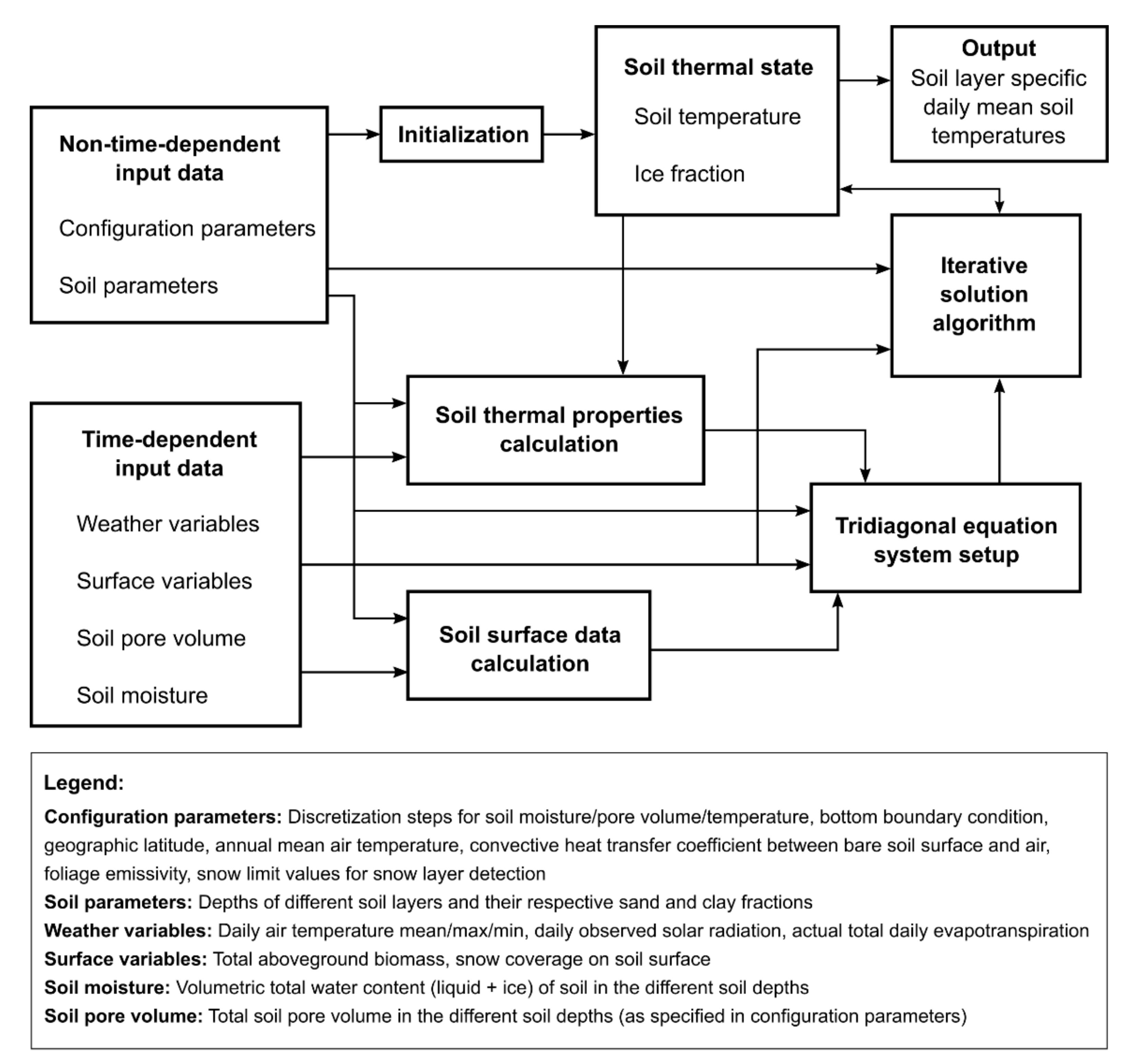
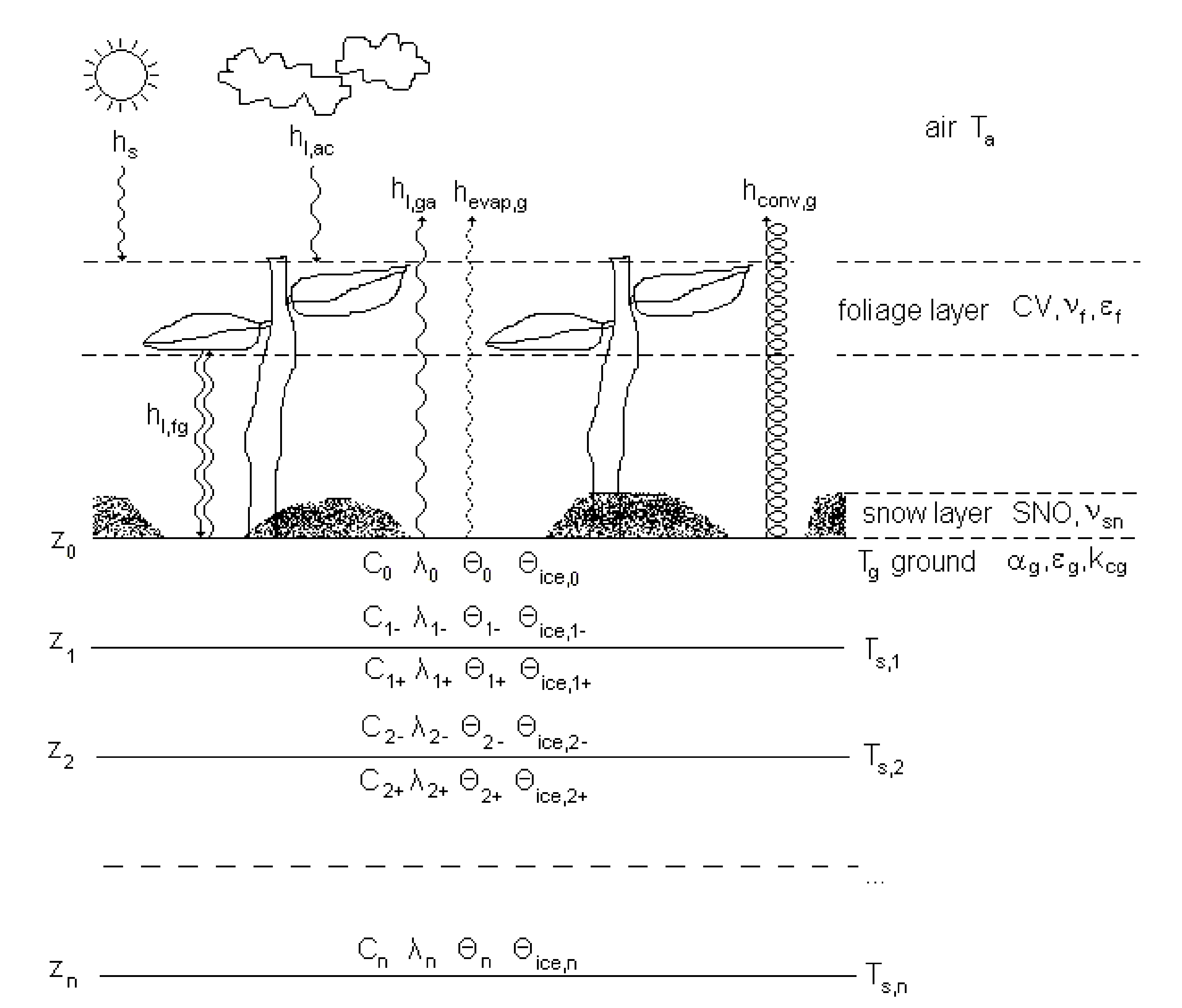
2.1. Model Description
2.1.1. Soil Surface Temperature: Vegetated Soil Surface without Snow Cover
2.1.2. Soil Surface Temperature: Soil Surface with Dense Snow Cover
2.1.3. Soil Surface Temperature: Soil Surface with Partial Snow Cover (General Case)
2.1.4. Subsurface Soil Temperature: Soil Temperature Equation in Finite-Difference Form
2.1.5. Subsurface Soil Temperature: Top and Bottom Boundary Conditions
- (i)
- To set the approximated daily mean heat flux at the bottom of the simulated soil profile to zero;
- (ii)
- To fix the temperature at the bottom of the soil profile to the annual mean air temperature TAA (°C), which is an input to the model; and
- (iii)
- To assume that the soil thermal properties λ and C and the ice content θice near the bottom of the soil profile are constant over z and t for depths z ≥ zmax and that the temperature at the bottom of the soil profile varies sinusoidally with a one-year period around a mean value of TAA. With the angular frequency of a year ωa (rad s−1) and the approximated damping depth at the bottom of the soil profile (m) for annual frequency, this leads to the following bottom boundary condition (detailed derivation can be found in Appendix C):
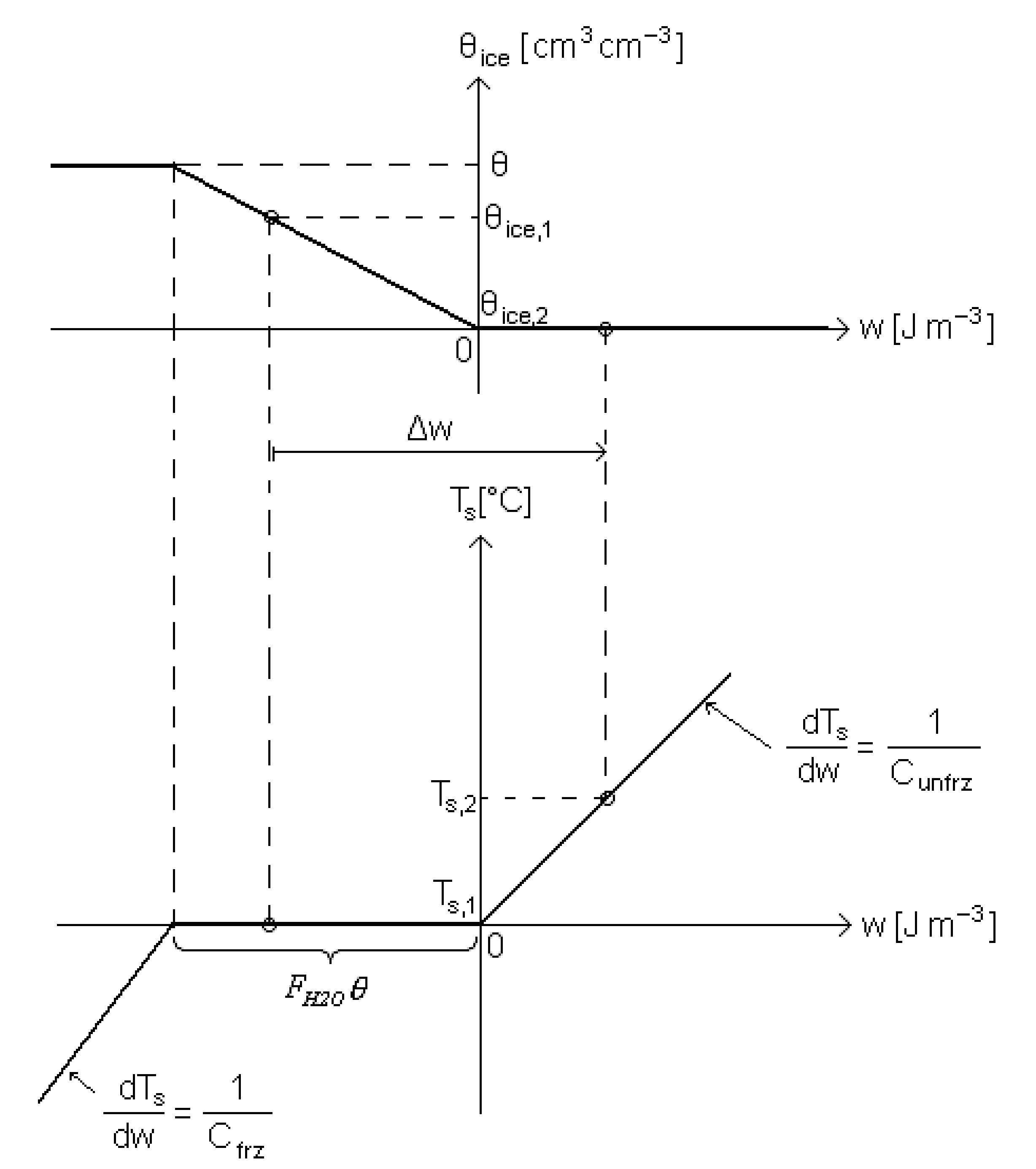
2.1.6. Subsurface Soil Temperature: Treatment of Freezing/Thawing of Soil Water
2.2. Calibration and Validation Sites
3. Results and Discussion
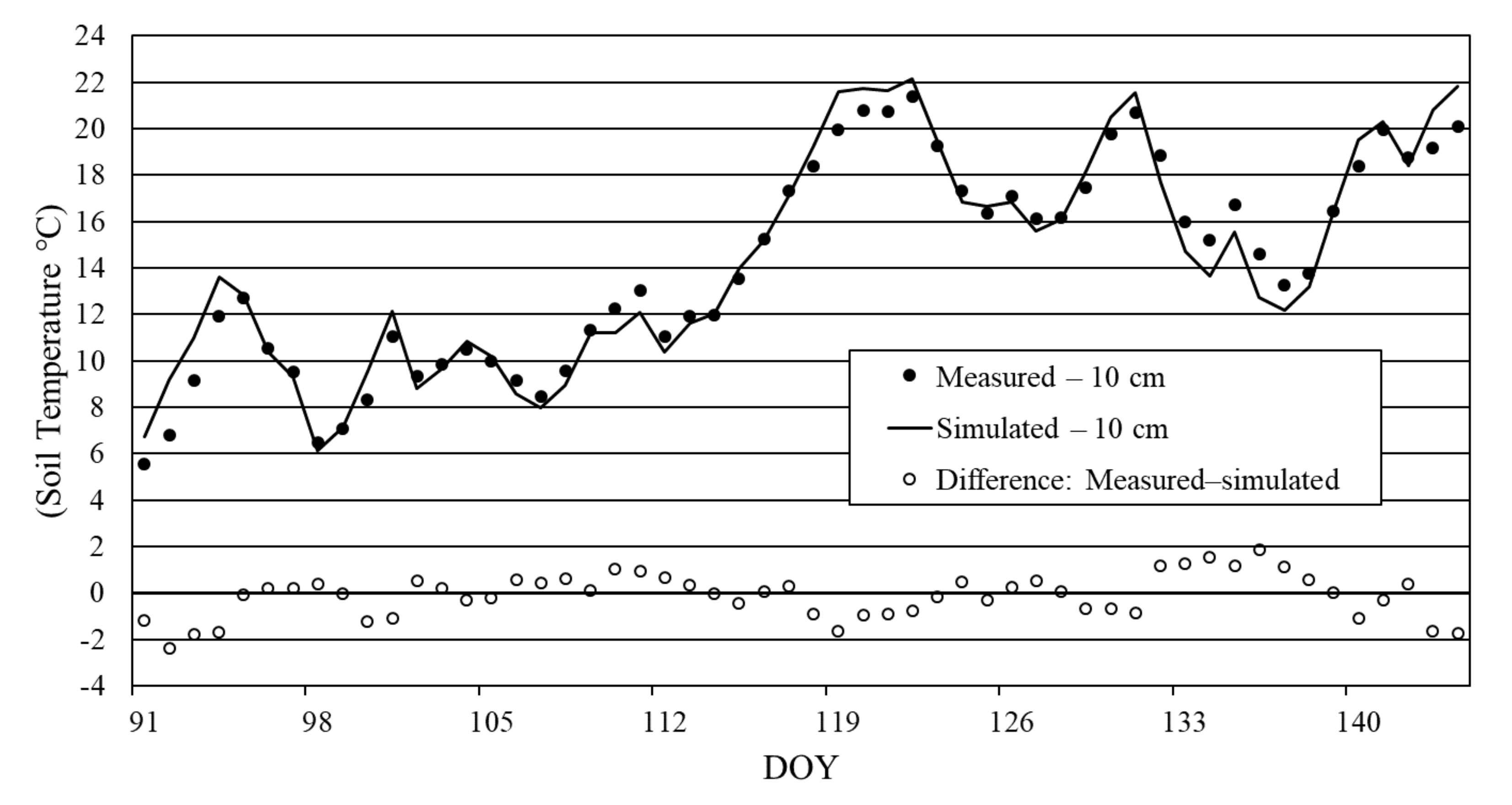
AGRISOTES Model Calibration, Validation and Sensitivity Analysis on Daily Mean Soil Temperatures
4. Conclusions
- (a)
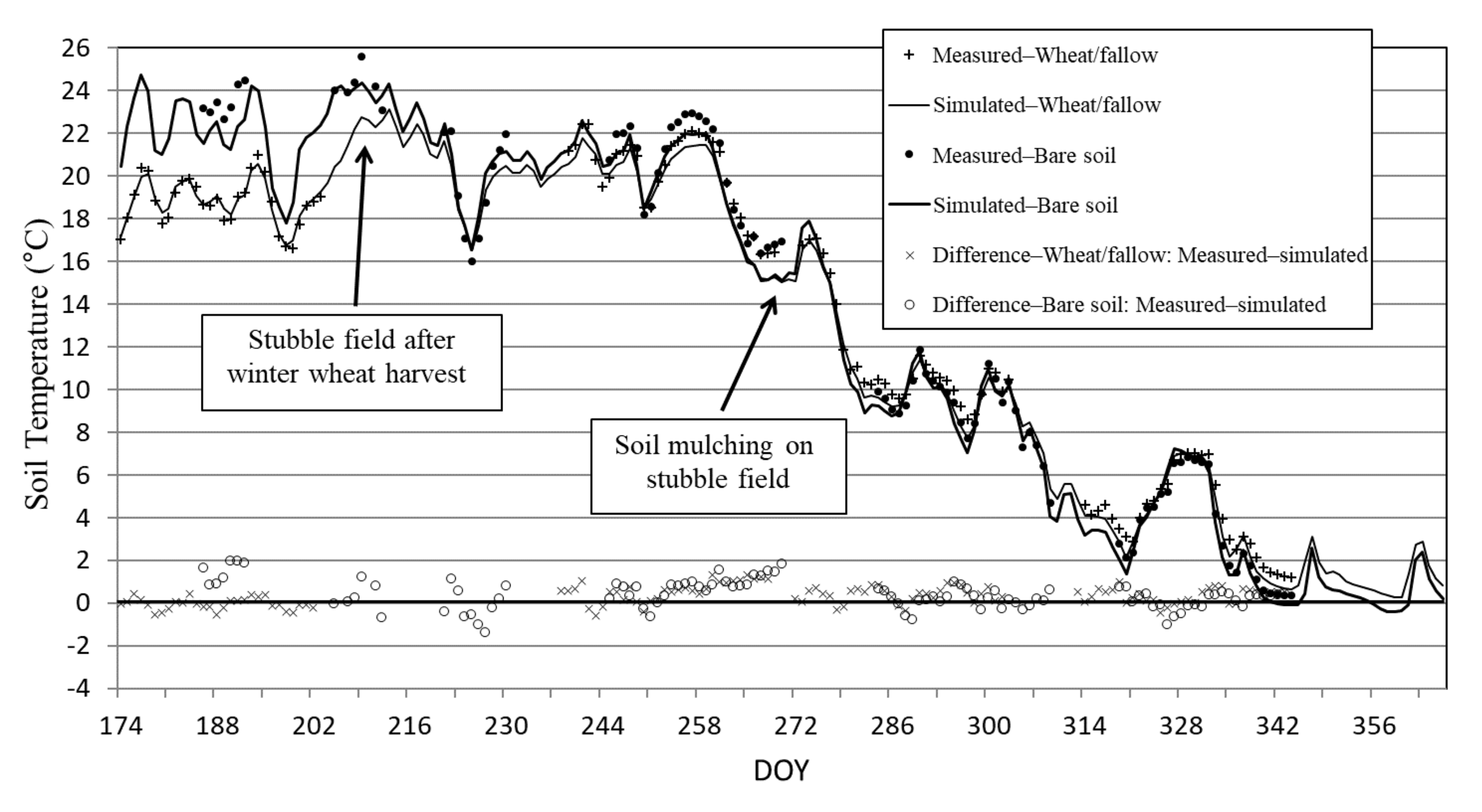
- is able to produce a smooth transition between bare soil and vegetated surface at the beginning of the vegetation period, as well as after sudden surface condition changes such as harvest;
- (b)
- represents the influence of surface biomass dynamics on soil temperatures with acceptable accuracy for many agricultural applications;
- (c)
- RMSE is higher for bare soil than for vegetated surfaces and intensively decreases with depth, indicating that the model is more sensitive to atmospheric forcing (a stronger effect on bare soil) than to the given soil characteristics and the parameterization of the energy transport over the whole profile;
- (d)
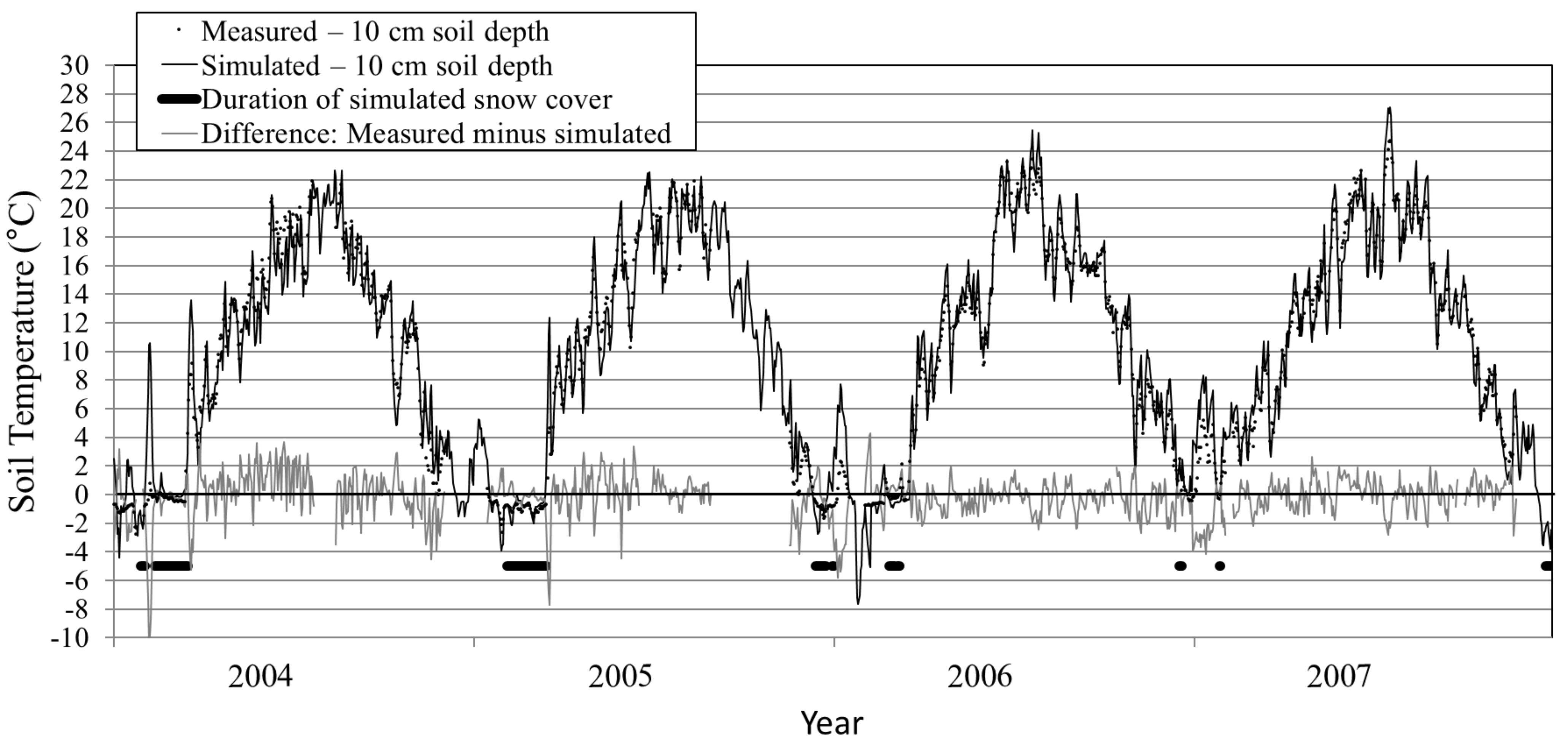
- is highly sensitive to the presence of snow cover; and
- (e)
- reflects well the most determining soil physical factors such as porosity, soil texture and soil water content. Soil surface conditions, however, remain the greatest influence under agricultural land use.
Author Contributions
Funding
Institutional Review Board Statement
Informed Consent Statement
Data Availability Statement
Acknowledgments
Conflicts of Interest
Appendix A. Incoming Atmospheric Longwave Radiation
Appendix B. Averaging Calculations for Top Boundary Condition during Snow-Free Periods
Appendix C. Derivation of Bottom Boundary Equations
Appendix D. Notations and Units
| Quantity | Unit | Description |
| Part I | ||
| C | J m−3 K−1 | volumetric soil heat capacity |
| CV | kg ha−1 | total aboveground biomass |
| da | m | damping depth for annual frequency |
| ETa | mm H2O | actual daily evapotranspiration |
| FH2O | J m−3 | latent heat of ice fusion related to volume of liquid water (≈3.34 ∙ 108 J m−3) |
| h | W m−2 | soil heat flow |
| hconv,g | W m−2 | convective heat transfer from the soil surface to the atmosphere |
| hevap | W m−2 | total evaporative heat transfer to the atmosphere per ground area |
| hevap,g | W m−2 | evaporative heat transfer from the soil surface to the atmosphere |
| hevap,mean | W m−2 | daily mean total evaporative heat transfer to the atmosphere per ground area |
| hl0 | W m−2 | long-wave radiation for a black body at air temperature |
| hl,ac | W m−2 | incoming atmospheric long-wave radiation |
| hl,fg | W m−2 | net long-wave radiation from the foliage to the ground (per total ground area) |
| hl,g0 | W m−2 | long-wave radiation from soil surface at air temperature |
| hl,g0,mean | W m−2 | daily mean long-wave radiation from soil surface at air temperature |
| hl,ga | W m−2 | outgoing thermal long-wave radiation emitted from the bare soil |
| hnet,g | W m−2 | net ground heat flow |
| hnet,g,mean | W m−2 | daily mean net ground heat flow |
| hs | W m−2 | observed solar radiation per unit area of ground surface |
| hs,clr | W m−2 | clear-sky irradiance |
| hs,clr,mean | W m−2 | daily mean clear-sky irradiance |
| hs,mean | W m−2 | daily mean observed solar radiation per unit area of ground surface |
| ht,1 | W m−2 | net incoming heat flux for snow-free periods |
| ht,1,mean | W m−2 | daily mean net incoming heat flux for snow-free periods |
| k1 | W m−2 K−1 | net heat transfer coefficient for snow-free periods |
| k1,mean | W m−2 K−1 | daily mean net heat transfer coefficient for snow-free periods |
| kcg | W m−2 K−1 | convective heat transfer coefficient from the soil surface to air |
| kl0 | W m−2 K−1 | derivate of black-body long-wave radiation with respect to temperature, evaluated at air temperature |
| kl0,mean | W m−2 K−1 | daily mean value of kl0 |
| kl,g0 | W m−2 K−1 | derivate of long-wave radiation from soil surface with respect to temperature, evaluated at air temperature |
| kl,g0,mean | W m−2 K−1 | daily mean value of kl,g0 |
| ksnow | 1 | damping factor for snow coverage |
| R1 | m2 K W−1 | thermal resistance respective ground heat flow for snow-free periods |
| R1,mean | m2 K W−1 | thermal resistance respective ground heat flow for snow-free periods, applicable to daily mean data |
| R2,mean | m2 K W−1 | thermal resistance respective ground heat flow for dense snow cover, applicable to daily mean data |
| Rmean | m2 K W−1 | thermal resistance respective ground heat flow for partial snow cover, applicable to daily mean data |
| SNO | mm H2O | snow water equivalent of snow layer |
| SNOlimit,1 | mm H2O | lower limit for SNO below which the snow layer is ignored |
| SNOlimit,2 | mm H2O | upper limit for SNO beyond which the snow layer is treated as dense |
| s | 1 | ratio of measured solar radiation to clear-sky irradiance |
| TAA | °C | annual mean air temperature |
| Ta | °C | air temperature (2 m height) |
| Ta,mean | °C | daily mean air temperature (2 m height) |
| Tg | °C | soil surface temperature |
| Tg,mean | °C | daily mean soil surface temperature |
| Ts | °C | soil temperature |
| t | s | time |
| VPclay | vol % | volume percentage of total solid soil matter that is clay |
| VPsand | vol % | volume percentage of total solid soil matter that is sand |
| w | J m−3 | heat energy density |
| z | m | depth in soil profile (z = 0 at soil surface, z > 0 inside the soil) |
| zmax | m | maximum simulation depth (bottom of soil profile) |
| Part II | ||
| αg | 1 | soil surface albedo (0–1) |
| β | ha kg−1 | parameter in νf(CV)-relation |
| ΔT1 | °C | difference between soil surface and air temperature during snow-free periods for zero ground heat flow |
| ΔT1,mean | °C | difference between daily mean soil surface and air temperature during snow-free periods for zero ground heat flow |
| ΔT2,mean | °C | difference between daily mean soil surface and air temperature for dense snow cover and zero ground heat flow |
| ΔTg | °C | difference between soil surface and air temperature |
| ΔTg,mean | °C | difference between daily mean soil surface and air temperature |
| ΔTmean | °C | difference between daily mean soil surface and air temperature for partial snow cover and zero ground heat flow |
| Δt | s | simulation time step (= 86,400 s) |
| εac | 1 | atmospheric emissivity (0–1) |
| εf | 1 | foliage emissivity (0–1) |
| εg | 1 | ground (soil surface) emissivity (0–1) |
| ζ | 1 | ice fraction (0–1) |
| θ | cm3 cm−3 | volumetric total soil water content (liquid + ice, but neglecting volume expansion of frozen water) |
| θice | cm3 cm−3 | volumetric ice content in soil, but neglecting volume expansion of frozen water |
| θsat | cm3 cm−3 | saturated volumetric water content or total soil pore volume |
| λ | W m−1 K−1 | soil thermal conductivity |
| μfg | 1 | radiation exchange degree between foliage and ground |
| νf | 1 | vegetation cover (0–1) |
| νsn | 1 | snow coverage factor (0–1) |
| σ | W m−2 K−4 | Stefan-Boltzmann constant (≈5.67 ∙ 10−8 W m−2 K−4) |
| ωa | rad s−1 | angular frequency of the year |
Appendix E

| Station Name | Station Code | Long | Lat | Altitude | Soil Description |
|---|---|---|---|---|---|
| ° | ° | m | |||
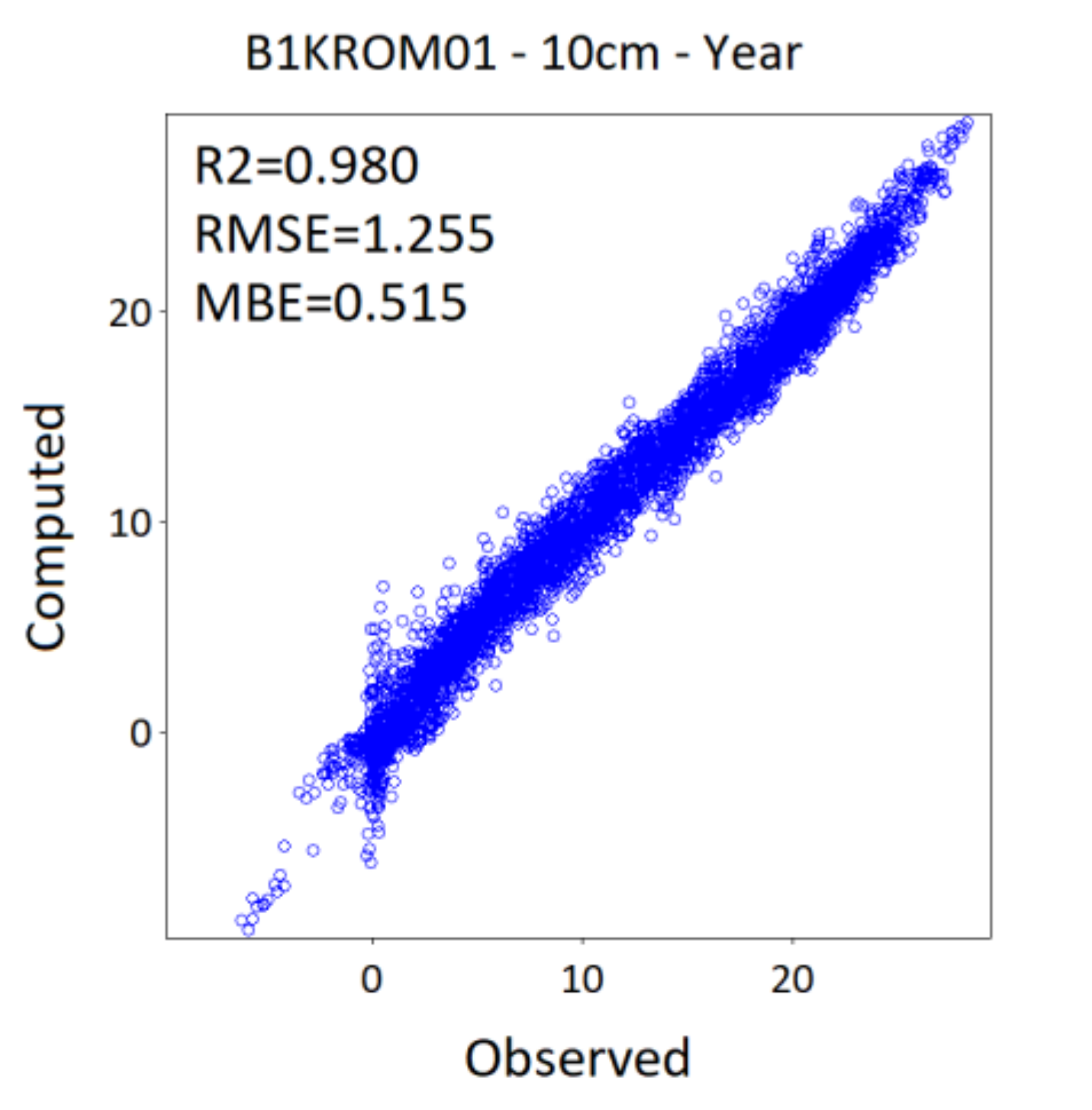
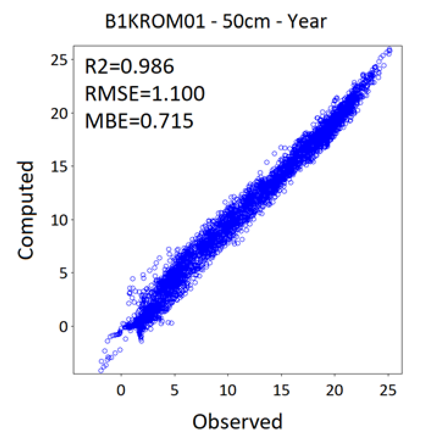
| KROMĚŘÍŽ | B1KROM01 | 17.3653 | 49.2847 | 233 | 0–100 cm loamy soil, chernozem |
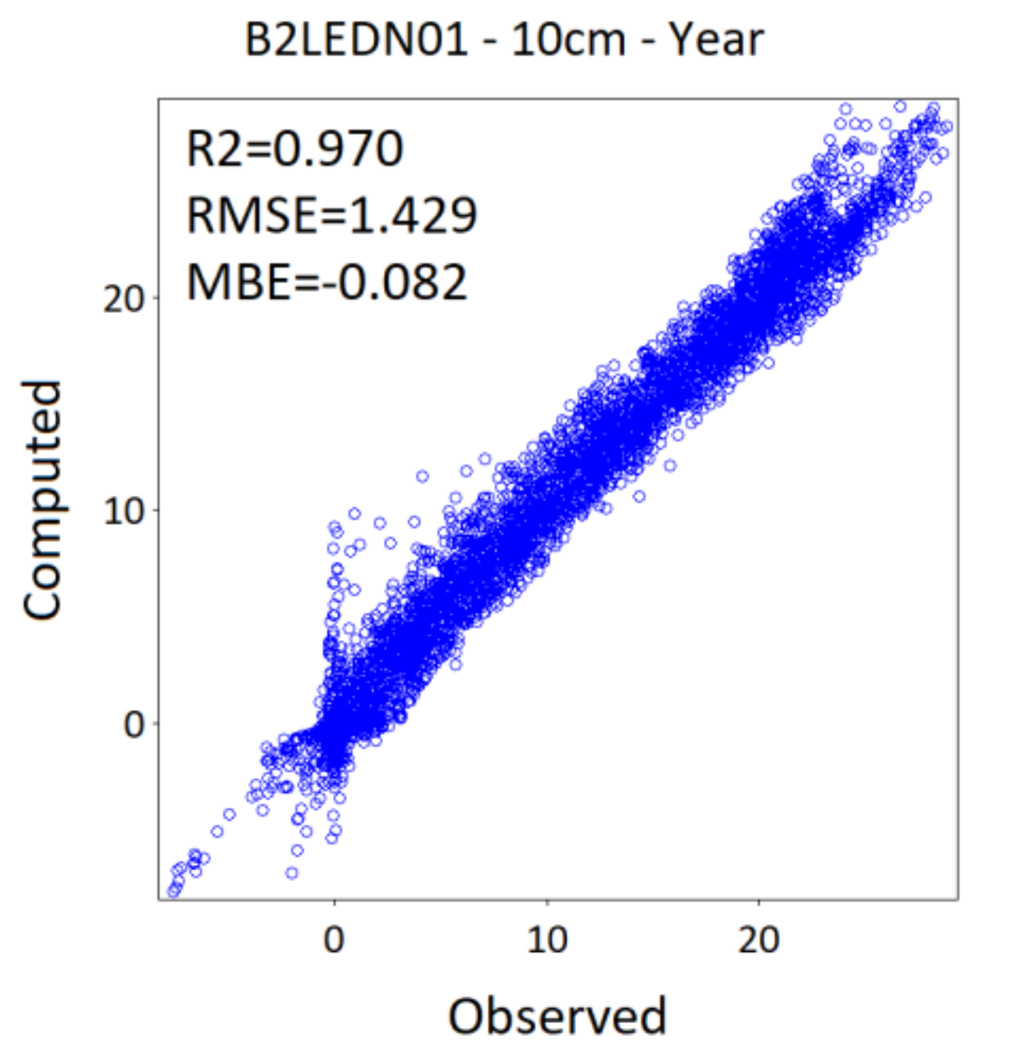
| LEDNICE | B2LEDN01 | 16.7989 | 48.79262 | 177 | 0–100 cm loamy soil, chernozem |
| KOCELOVICE | C1KOCE01 | 13.83861 | 49.46722 | 519 | 0–25 cm sandy loam, 25–50 cm loam 50–100 cm sandy, Cambisol |
| UPICE | H1UPIC01 | 16.01162 | 50.50642 | 413 | 0–70 cm loamy-sand |
| BĚLOTÍN | O1BELO01 | 17.8042 | 49.5869 | 306 | 0–100 cm loamy soil, luvisol |
| LUČINA | O1LUCI01 | 18.4425 | 49.7308 | 300 | 0–100 cm loam. Pseudogleyic luvisol |
| LUKÁ | O2LUKA01 | 16.95333 | 49.65222 | 510 | 0–30 cm sandy-loam 30–100 cm loam, Cambisol |
| USTÍ NAD LABEM | U1ULKO01 | 14.04111 | 50.68333 | 375 | 0–30 cm sandy loam 30–100 cm loam, typical Cambisol with strong human influence |
| LIBEREC | U2LIBC01 | 15.02389 | 50.76972 | 398 | 0–22 cm sandy-loam 22–100 cm loam, gleyic soil |
| Surface conditions: All measurement sites are characterized by no or only negligible slope inclination (flat area) and grass cover with regular mowing; AGRISOTES simulations were carried out with constant surface biomass of 1000 kg ha−1 (representing short grass). | |||||
| Station Name | Station Code | Soil Depth 10 cm | Soil Depth 50 cm | ||||
|---|---|---|---|---|---|---|---|
| R2 | RMSE | MBE | R2 | RMSE | MBE | ||
| °C | °C | °C | °C | ||||
| KROMĚŘÍŽ | B1KROM01 | 0.98 | 1.26 | 0.52 | 0.99 | 1.10 | 0.72 |
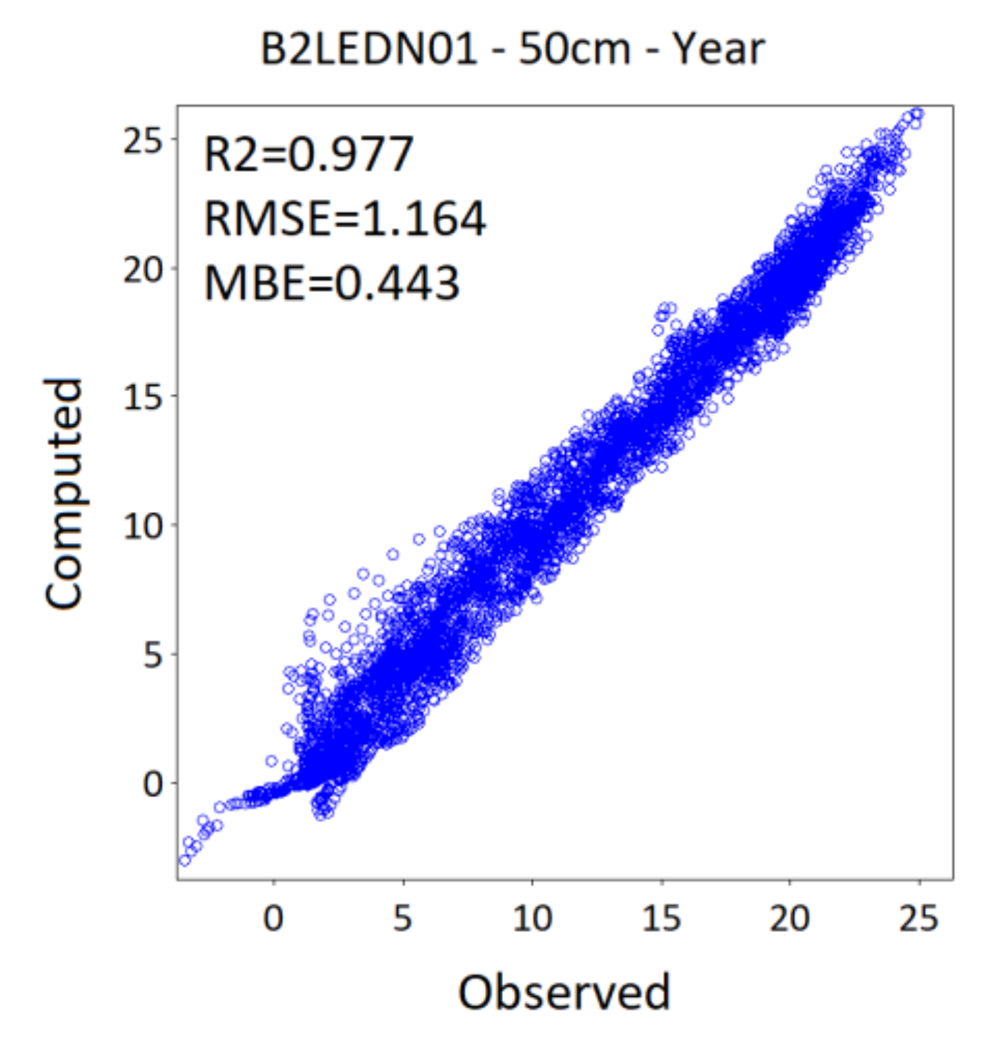
| LEDNICE | B2LEDN01 | 0.97 | 1.43 | −0.08 | 0.98 | 1.16 | 0.44 |
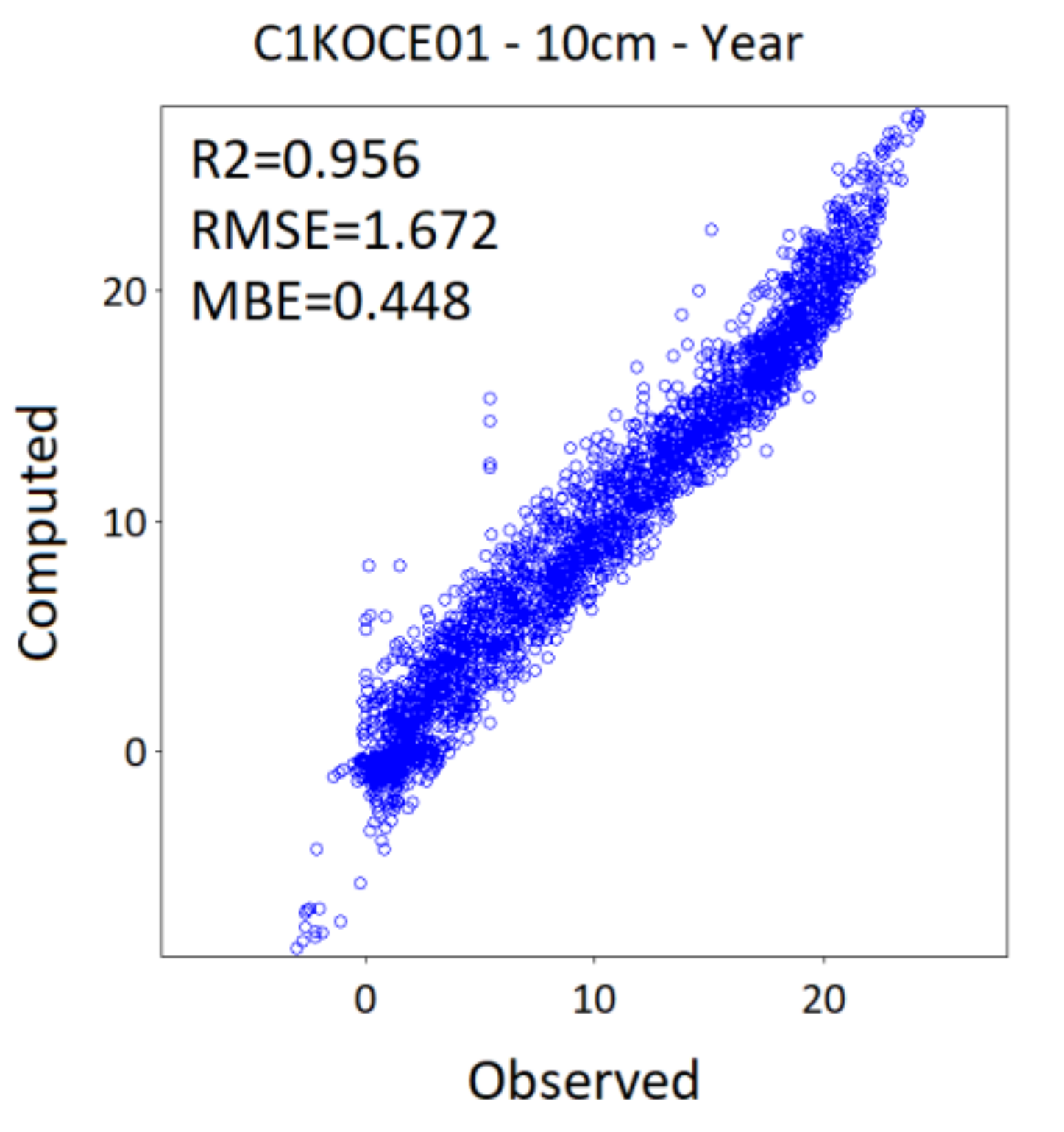
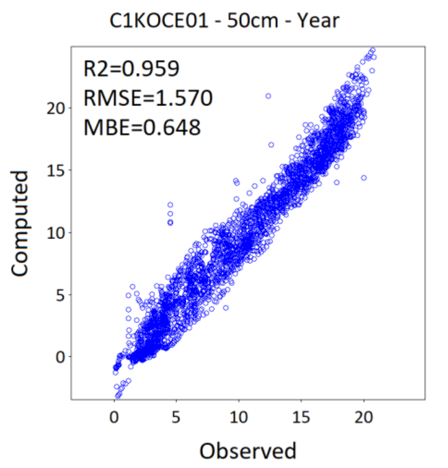
| KOCELOVICE | C1KOCE01 | 0.96 | 1.67 | 0.45 | 0.96 | 1.57 | 0.65 |
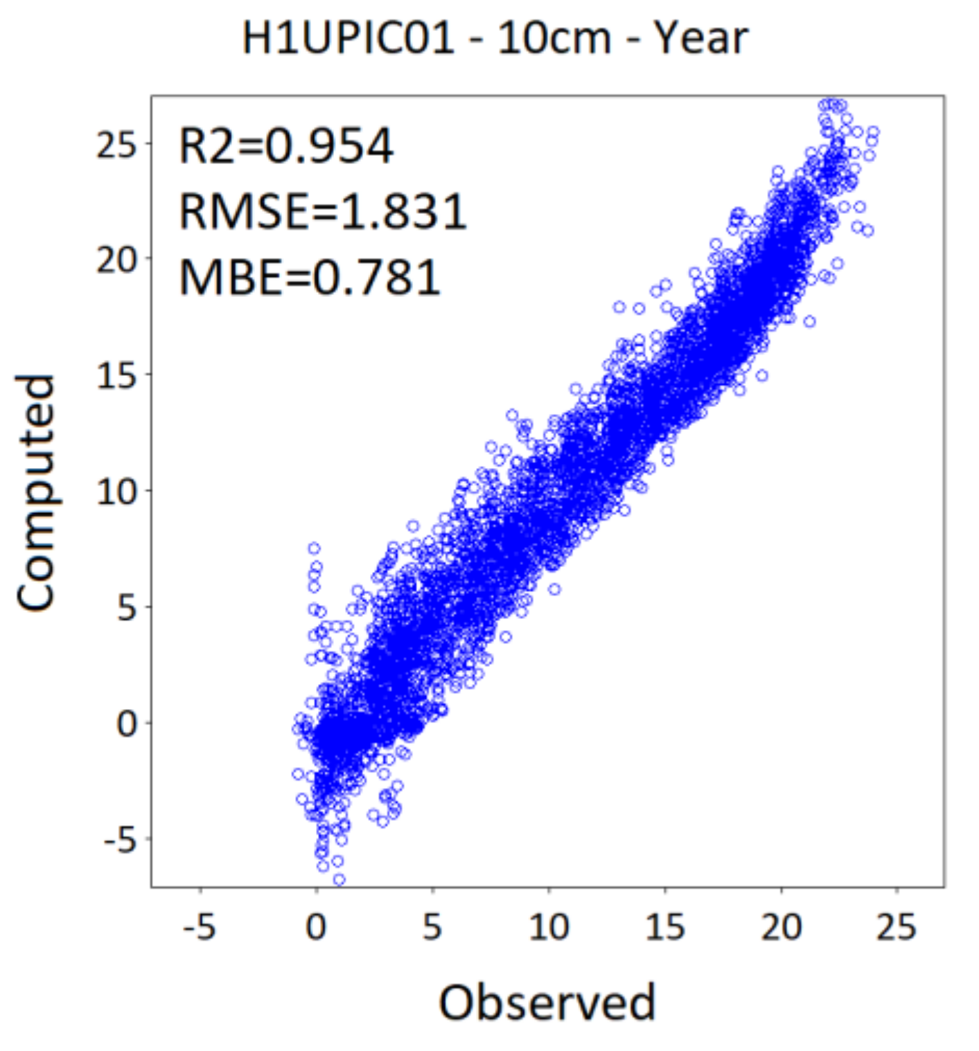
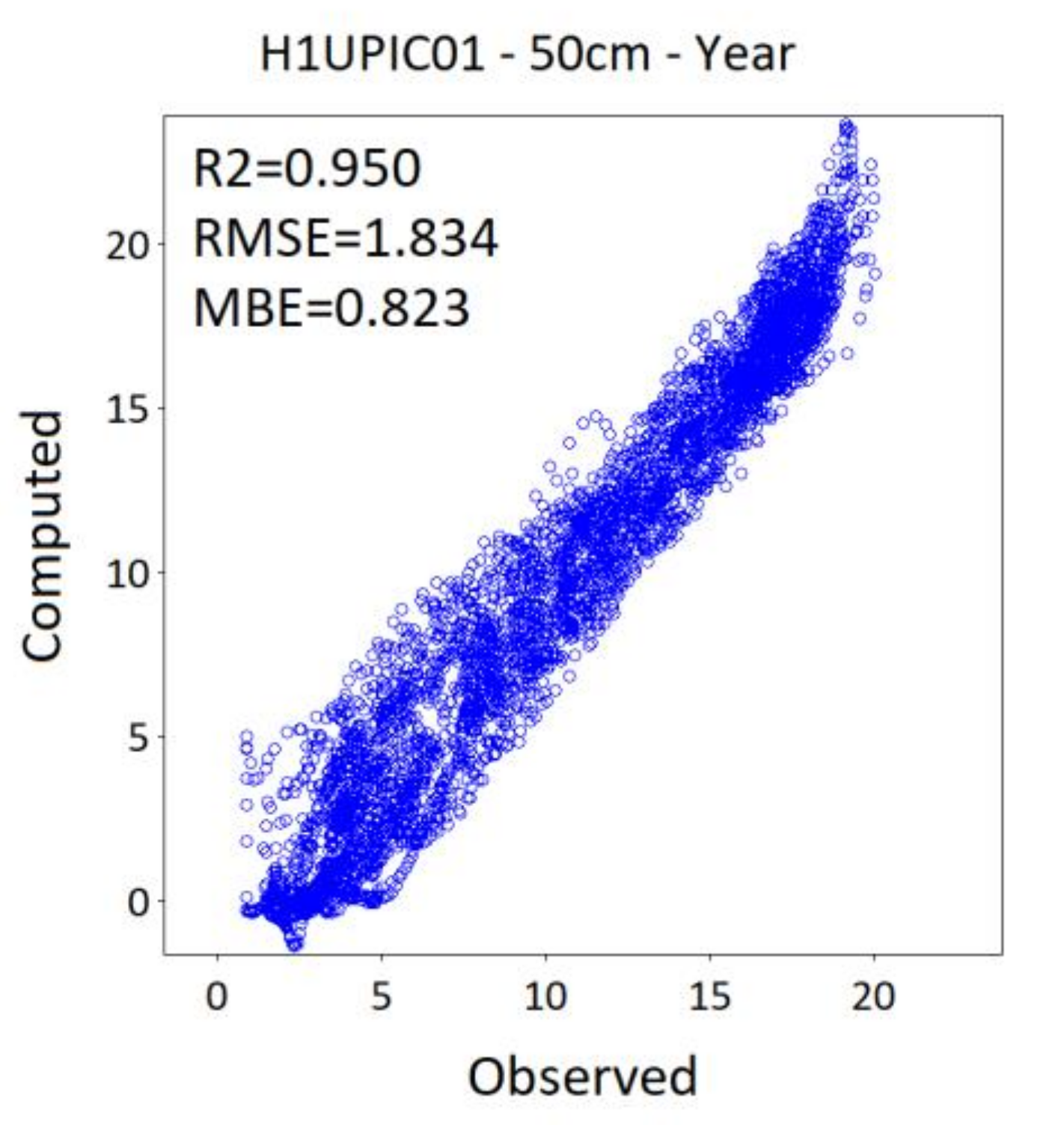
| UPICE | H1UPIC01 | 0.95 | 1.83 | 0.78 | 0.95 | 1.83 | 0.82 |
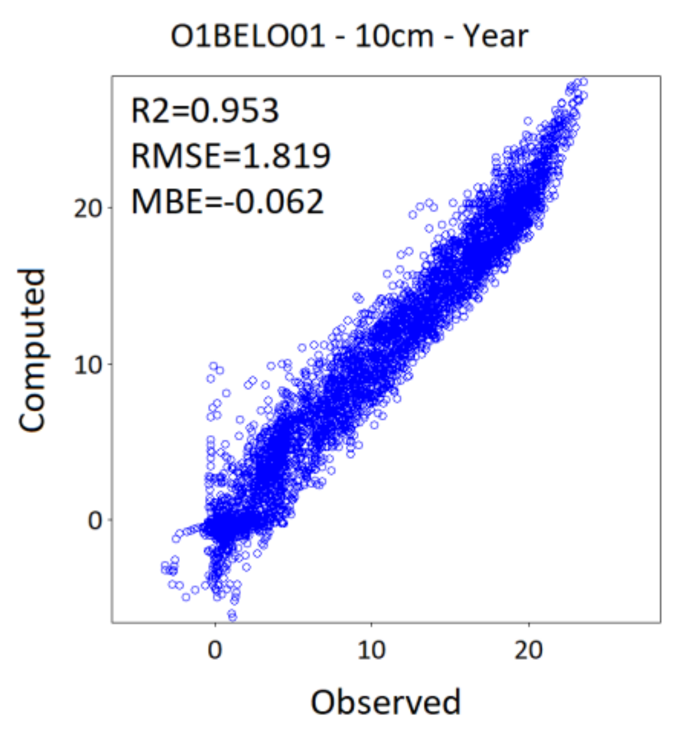
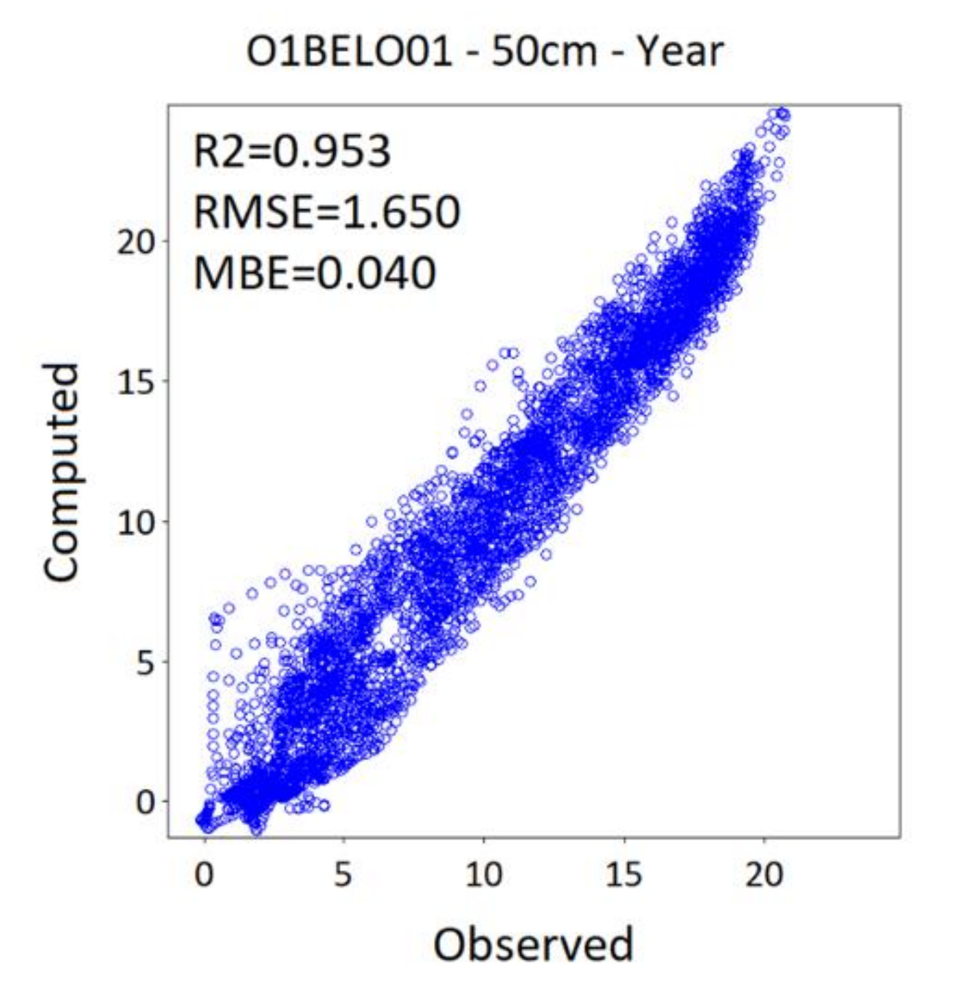
| BĚLOTÍN | O1BELO01 | 0.95 | 1.82 | −0.06 | 0.95 | 1.65 | 0.04 |
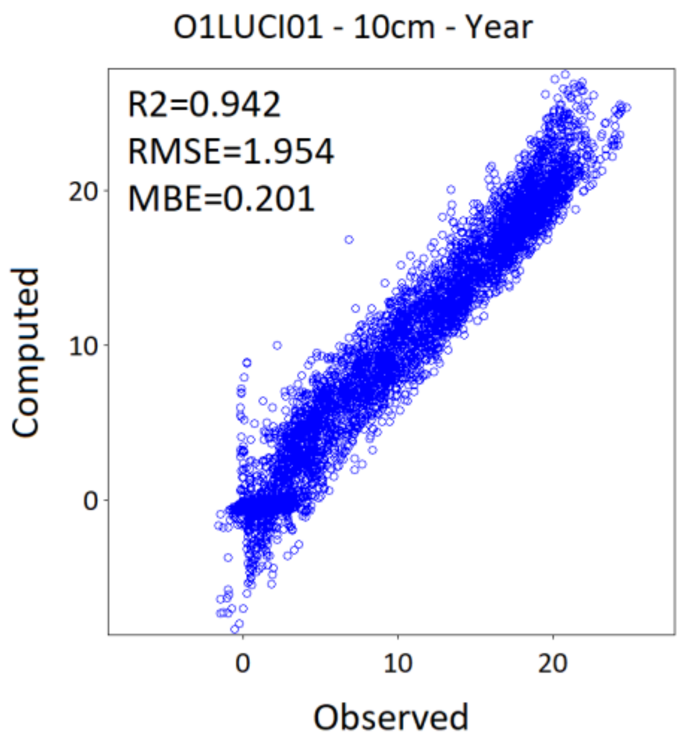
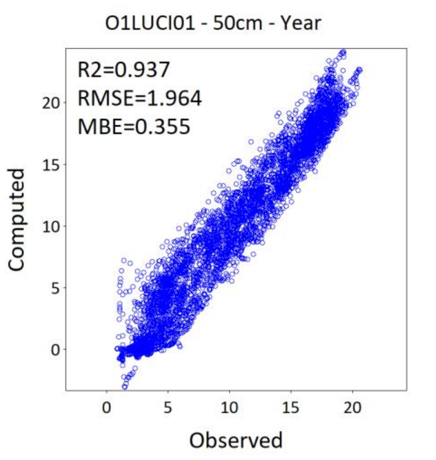
| LUČINA | O1LUCI01 | 0.94 | 1.95 | 0.20 | 0.94 | 1.96 | 0.36 |
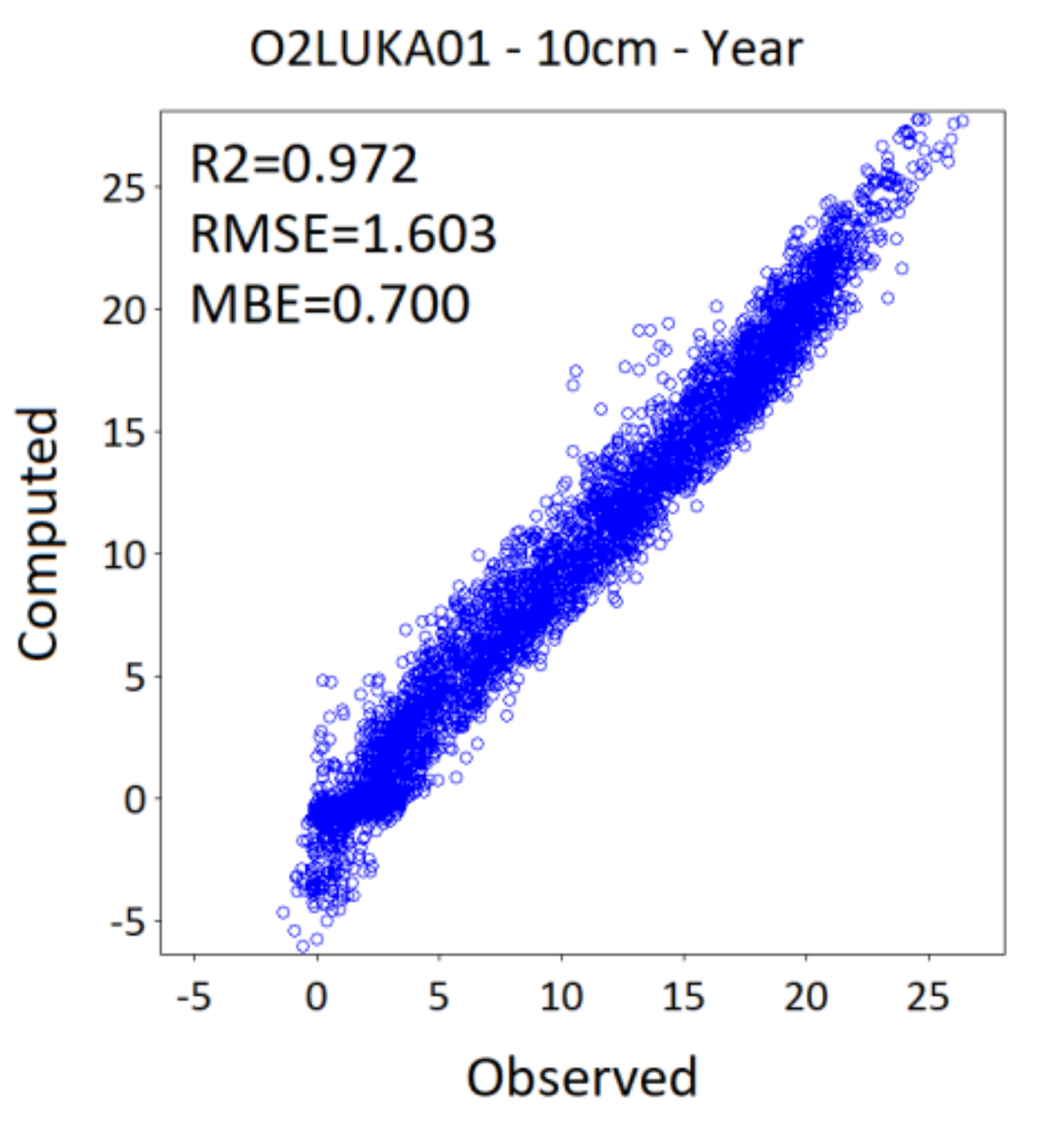
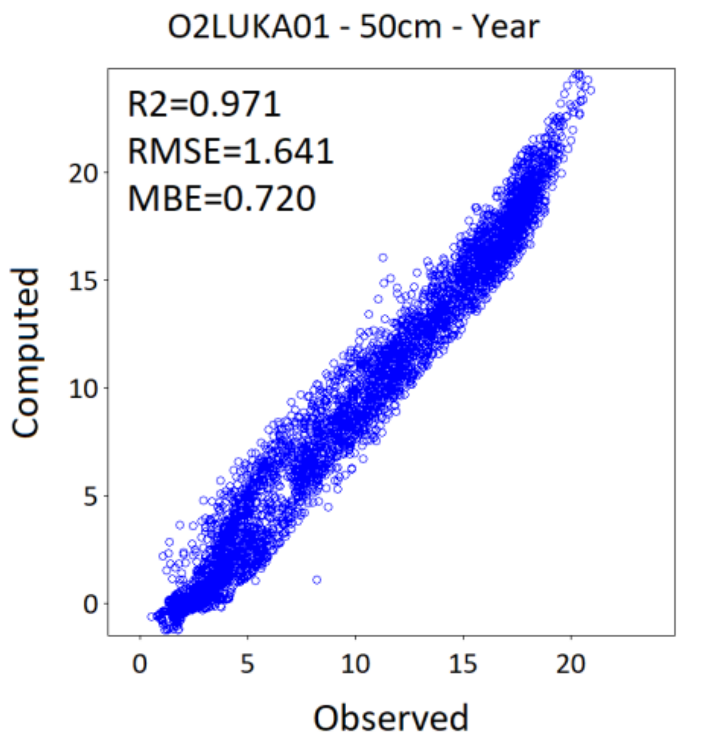
| LUKÁ | O2LUKA01 | 0.97 | 1.60 | 0.70 | 0.97 | 1.64 | 0.72 |
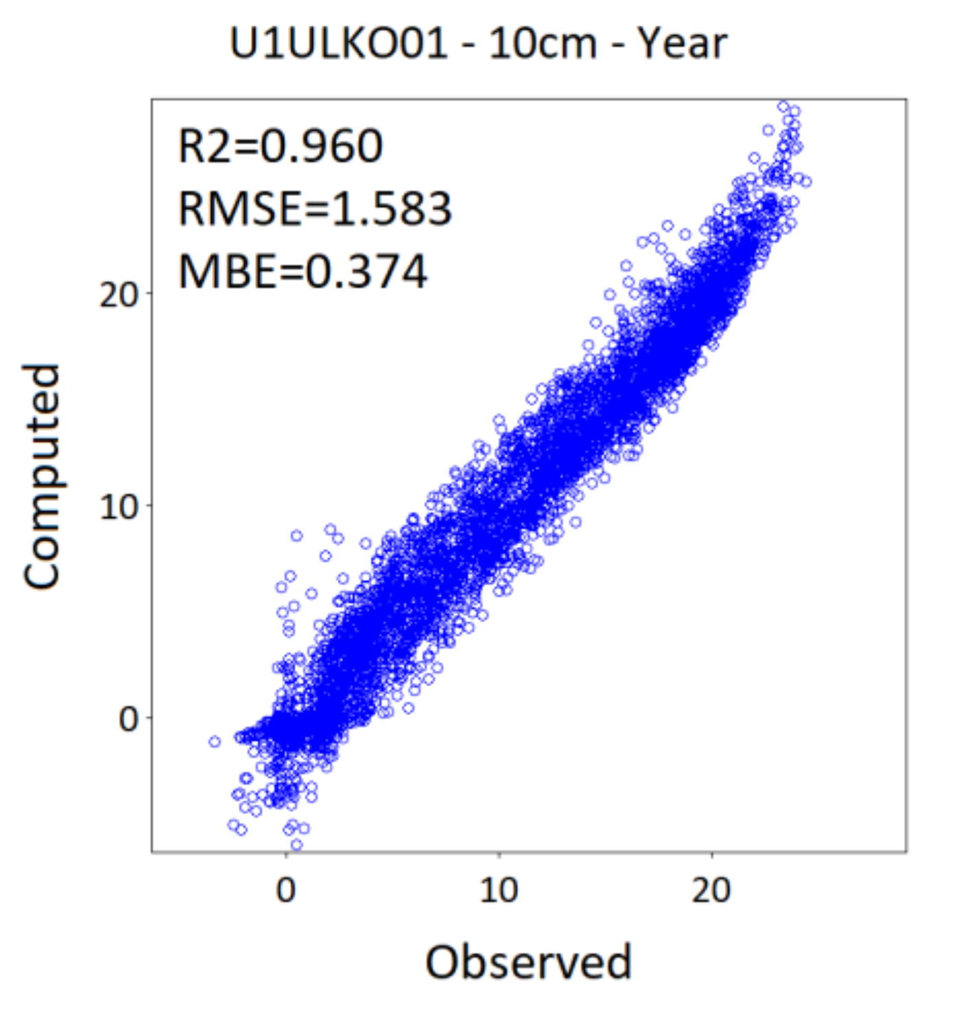
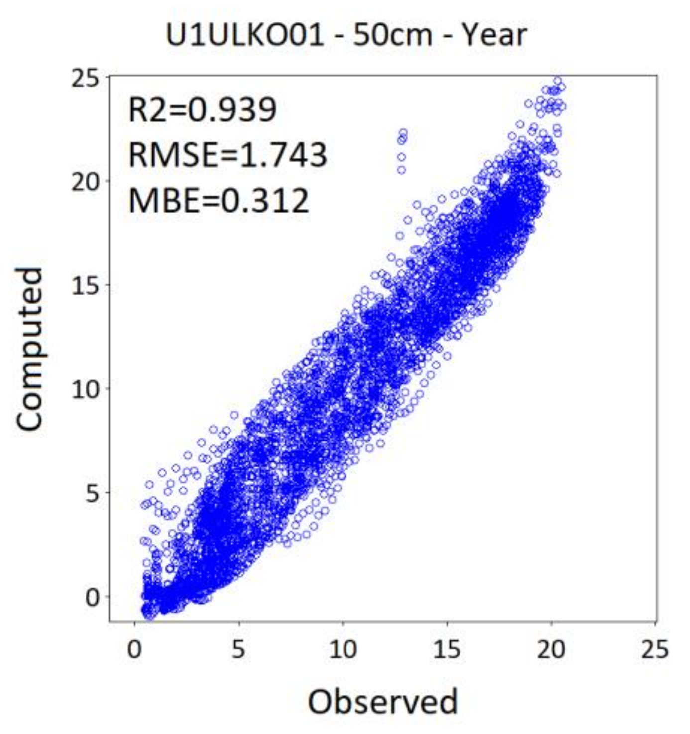
| USTÍ NAD LABEM | U1ULKO01 | 0.96 | 1.58 | 0.37 | 0.94 | 1.74 | 0.31 |
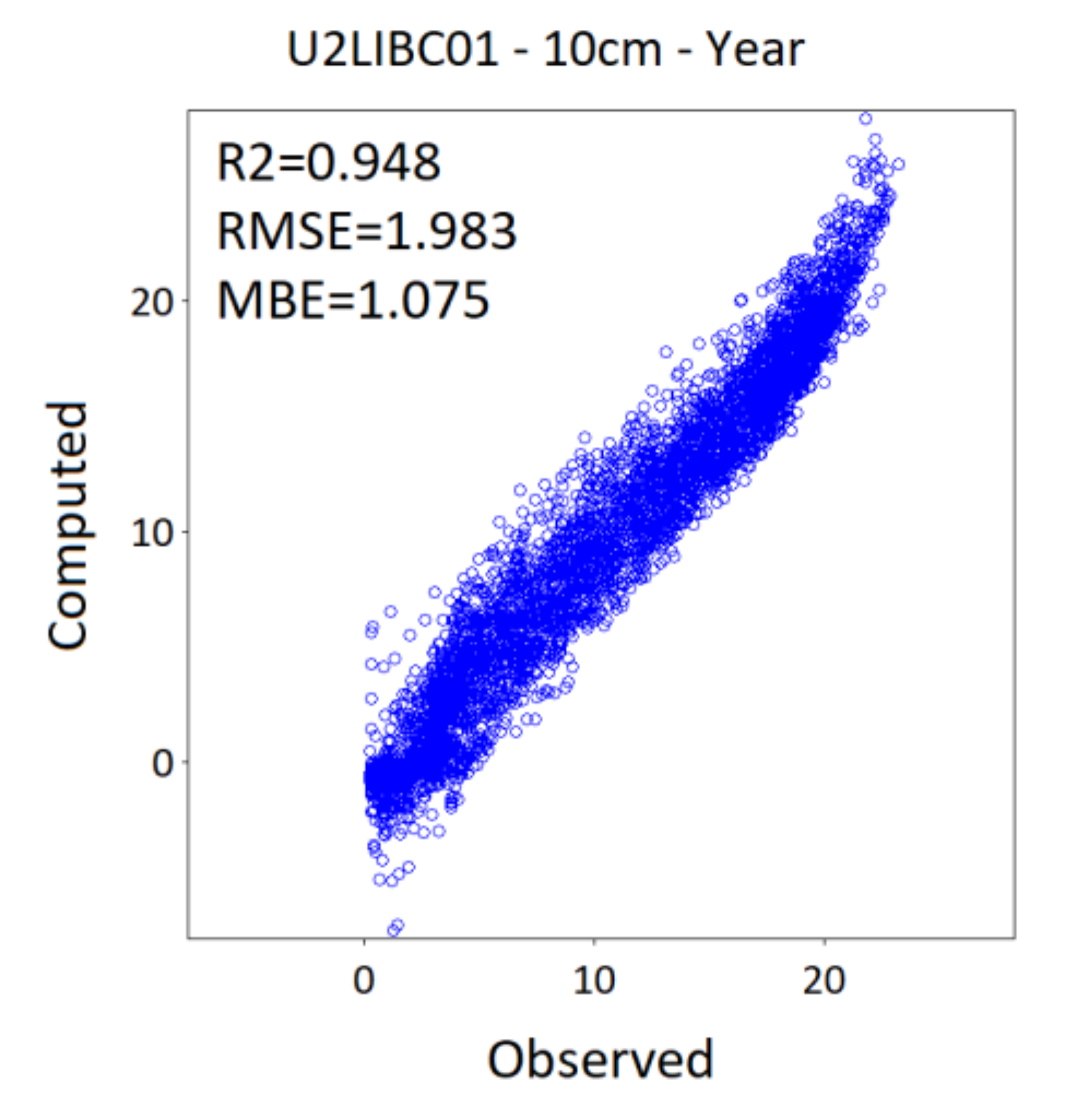
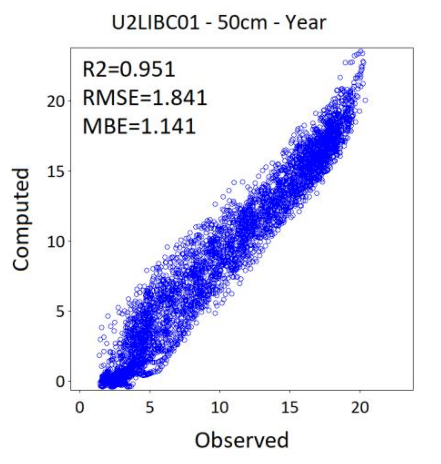
| LIBEREC | U2LIBC01 | 0.95 | 1.98 | 1.08 | 0.95 | 1.84 | 1.14 |


Appendix F. Software/Data Availability of AGRISOTES
References
- Dokuchaev, V.V. Russian Chernozem—Selected Works of V.V. Dokuchaev; Israel Program for Scientific Translations: Jerusalem, Israel, 1967. [Google Scholar]
- Fanning, D.S.; Fanning, M.C.B. Soil Morphology, Genesis, and Classification; John Wiley and Sons: New York, NY, USA, 1989; 395p, ISBN 0471892483. [Google Scholar]
- Ellenberg, H. Zeigerwerte der Gefäßpflanzen Mitteleuropas. Scr. Geobot. 1974, 9, 1–97. [Google Scholar]
- Gray, J.M.; Humphreys, G.S.; Deckers, J.A. Relationships in soil distribution as revealed by a global soil database. Geoderma 2009, 150, 309–323. [Google Scholar] [CrossRef]
- Larcher, W. Physiological Plant Ecology, 4th ed.; Springer: Berlin, Germany, 2003; 513p, ISBN 978-3-540-43516-7. [Google Scholar]
- Trnka, M.; Kersebaum, K.C.; Eitzinger, J.; Hayes, M.; Hlavinka, P.; Svoboda, M.; Dubrovský, M.; Semerádová, D.; Wardlow, B.; Pokorný, E.; et al. Consequences of climate change for the soil climate in Central Europe and the central plains of the United States. Clim. Chang. 2013, 120, 405–418. [Google Scholar] [CrossRef] [Green Version]
- Davis, P.M.; Brenes, N.; Allee, L.L. Temperature dependent models to predict regional differences in corn rootworm (Coleoptera: Chrysomelidae) phenology. Environ. Entomol. 1996, 25, 767–775. [Google Scholar] [CrossRef]
- Orchard, V.A.; Cook, F.J. Relationship between soil respiration and soil moisture. Soil Biol. Biochem. 1983, 15, 447–453. [Google Scholar] [CrossRef]
- Parton, W.J.; Schimel, D.S.; Cole, C.V.; Ojima, D.S. Analysis of factors controlling soil organic matter levels in Great Plains grasslands. Soil Sci. Soc. Am. J. 1987, 51, 1173–1179. [Google Scholar] [CrossRef]
- Parton, W.J.; Stewart, J.W.B.; Cole, C.V. Dynamics of C, N, P and S in grassland soils: A model. Biogeochemistry 1988, 5, 109–131. [Google Scholar] [CrossRef]
- Parton, W.J.; Mosier, A.R.; Ojima, D.S.; Valentine, D.W.; Schimel, D.S.; Weier, K.; Kulmala, A.E. Generalized model for N2 and N2O production from nitrification and denitrification. Glob. Biogeochem. Cycles 1996, 10, 401–412. [Google Scholar] [CrossRef]
- Peterjohn, W.T.; Melillo, J.M.; Steudler, P.A.; Newkirk, K.M.; Bowles, F.P.; Aber, J.D. Responses of trace gas fluxes and N availability to experimentally elevated soil temperatures. Ecol. Appl. 1994, 4, 617–625. [Google Scholar] [CrossRef]
- Fu, C.; Lee, X.; Griffis, T.J.; Wang, G.; Wei, Z. Influences of root hydraulic redistribution on N2O emissions at AmeriFlux sites. Geophys. Res. Lett. 2018, 45, 5135–5143. [Google Scholar] [CrossRef]
- Rodrigo, A.; Recous, S.; Neel, C.; Mary, B. Modelling temperature and moisture effects on C–N transformations in soils: Comparison of nine models. Ecol. Modell. 1997, 102, 325–339. [Google Scholar] [CrossRef]
- Franko, U.; Oelschlägel, B.; Schenk, S. Simulation of temperature-, water- and nitrogen dynamics using the model CANDY. Ecol. Modell. 1995, 81, 213–222. [Google Scholar] [CrossRef]
- Qin, Y.; Bai, Y.; Chen, G.; Liang, Y.; Li, X.; Wen, B.; Lu, X.; Li, X. The effects of soil freeze–thaw processes on water and salt migrations in the western Songnen Plain, China. Sci. Rep. 2021, 11, 3888. [Google Scholar] [CrossRef]
- Wang, J.; Quan, Q.; Chen, W.; Tian, D.; Ciais, P.; Crowther, T.W.; Mack, M.C.; Poulter, B.; Tian, H.; Luo, Y.; et al. Increased CO2 emissions surpass reductions of non-CO2 emissions more under higher experimental warming in an alpine meadow. Sci. Total Environ. 2021, 769, 144559. [Google Scholar] [CrossRef]
- Bogomolov, V.Y.; Dyukarev, E.A.; Stepanenko, V.M.; Drozdov, E.D. Modeling the temperature and humidity conditions of mineral soils in an active layer model taking into account in depth changes in the thermodynamic properties of the soil. IOP Conf. Ser. Earth Environ. Sci. 2020, 611, 012012. [Google Scholar] [CrossRef]
- Kiselev, M.V.; Voropay, N.N.; Dyukarev, E.A.; Preis, Y.I. Temperature regimes of drained and natural peatlands in arid and water-logged years. IOP Conf. Ser. Earth Environ. Sci. 2019, 386, 012029. [Google Scholar] [CrossRef]
- Koçak, K.; Şaylan, L.; Eitzinger, J. Nonlinear prediction of near-surface temperature via univariate and multivariate time series embedding. Ecol. Modell. 2004, 173, 1–7. [Google Scholar] [CrossRef]
- Tanaka, K.; Hashimoto, S. Plant canopy effects on soil thermal and hydrological properties and soil respiration. Ecol. Modell. 2006, 196, 32–44. [Google Scholar] [CrossRef]
- Sepaskhah, A.R.; Boersma, L. Thermal conductivity of soils as a function of temperature and water content. Soil Sci. Soc. Am. J. 1979, 43, 439–444. [Google Scholar] [CrossRef]
- Dhanush, K.V.; Patil, D.R. Effect of mulches on soil moisture, temperature, weed suppression and estimation of cost benefit ratio of grape (Vitis vinifera L.) ‘Kishmish Rozavis White’ in northern dry zone of Karnataka, India. Acta Hortic. 2020, 1299, 61–66. [Google Scholar] [CrossRef]
- Gupta, S.C.; Larson, W.E.; Allmaras, R.R. Predicting soil temperature and soil heat flux under different tillage-surface residue conditions. Soil Sci. Soc. Am. J. 1984, 48, 223–232. [Google Scholar] [CrossRef]
- Zapata, D.; Rajan, N.; Mowrer, J.; Casey, K.; Schnell, R.; Hons, F. Long-term tillage effect on with-in season variations in soil conditions and respiration from dryland winter wheat and soybean cropping systems. Sci. Rep. 2021, 11, 2344. [Google Scholar] [CrossRef] [PubMed]
- Du, K.; Li, F.; Qiao, Y.; Leng, P.; Li, Z.; Ge, J.; Yang, G. Influence of no-tillage and precipitation pulse on continuous soil respiration of summer maize affected by soil water in the North China Plain. Sci. Total Environ. 2021, 766, 144384. [Google Scholar] [CrossRef] [PubMed]
- Huang, F.; Ding, X.; Li, W.; Jia, H.; Wei, X.; Zhao, X. The effect of temperature on the decomposition of different parts of maize residues in a solonchak. Catena 2021, 201, 105207. [Google Scholar] [CrossRef]
- Von Haden, A.C.; Marín-Spiotta, E.; Jackson, R.D.; Kucharik, C.J. Soil microclimates influence annual carbon loss via heterotrophic soil respiration in maize and switchgrass bioenergy cropping systems. Agric. For. Meteorol. 2019, 279, 107731. [Google Scholar] [CrossRef]
- Al-Maliki, S.; Al-Taey, D.K.A.; Al-Mammori, H.Z. Soil microbes, organic carbon protection and plant production in consideration with earthworms: A review. Plant Cell Biotechnol. Mol. Biol. 2020, 21, 99–125. [Google Scholar]
- Johnson, S.N.; Zhang, X.; Crawford, J.W.; Gregory, P.J.; Young, I.M. Egg hatching and survival time of soil-dwelling insect larvae: A partial differential equation model and experimental validation. Ecol. Modell. 2007, 202, 493–502. [Google Scholar] [CrossRef]
- Dai, Z.; Hu, J.; Fan, J.; Fu, W.; Wang, H.; Hao, M. No-tillage with mulching improves maize yield in dryland farming through regulating soil temperature, water and nitrate-N. Agric. Ecosyst. Environ. 2021, 309, 107288. [Google Scholar] [CrossRef]
- Liu, Z.; Lei, N. Effect of different tillage managements on soil physicochemical properties and crop yield. IOP Conf. Ser. Earth Environ. Sci. 2019, 384, 012175. [Google Scholar] [CrossRef]
- Eitzinger, J.; Parton, W.J.; Hartman, M. Improvement and validation of a daily soil temperature submodel for freezing/thawing periods. Soil Sci. 2000, 165, 525–534. [Google Scholar] [CrossRef]
- Zhang, T. Influence of the seasonal snow cover on the ground thermal regime: An overview. Rev. Geophys. 2005, 43, RG4002. [Google Scholar] [CrossRef]
- Ren, J.P.; Vanapalli, S.K.; Han, Z. Soil freezing process and different expressions for the soil-freezing characteristic curve. Sci. Cold Arid Reg. 2017, 9, 221–228. [Google Scholar]
- Balsamo, G. Land surface processes. In Proceedings of the ECMWF Workshop on Sub-Seasonal Predictability, Reading, UK, 2–5 November 2015; Available online: https://www.ecmwf.int/sites/default/files/elibrary/2015/14483-land-surface-processes.pdf (accessed on 9 March 2021).
- Dutra, E.; Balsamo, G.; Viterbo, P.; Miranda, P.M.A.; Beljaars, A.; Schär, C.; Elder, K. An improved snow scheme for the ECMWF land surface model: Description and offline validation. J. Hydrometeorol. 2010, 11, 899–916. [Google Scholar] [CrossRef]
- Trigo, I.F.; Boussetta, S.; Viterbo, P.; Balsamo, G.; Beljaars, A.; Sandu, I. Comparison of model land skin temperature with remotely sensed estimates and assessment of surface-atmosphere coupling. J. Geophys. Res. Atmos. 2015, 120, 12096–12111. [Google Scholar] [CrossRef] [Green Version]
- Sellers, P.J.; Mintz, Y.; Sud, Y.C.; Dalcher, A. A simple biosphere model (SiB) for use within general circulation models. J. Atmos. Sci. 1986, 43, 505–531. [Google Scholar] [CrossRef] [Green Version]
- Ek, M.; Mahrt, L. A User Guide to OSU1DPBL Version 1.0.4: A One-Dimensional Planetary Boundary Layer Model with Interactive Soil Layers and Plant Canopy; Department of Atmospheric Sciences, Oregon State University: Corvallis, OR, USA, 1991. [Google Scholar]
- Grünhage, L.; Haenel, H.-D. Detailed documentation of the PLATIN (PLant-ATmosphere INteraction) model. Landbauforsch. Völkenrode Sonderh. 2008, 319, 1–85. [Google Scholar]
- Walker, B.H.; Langridge, J.L. Modelling plant and soil water dynamics in semi-arid ecosystems with limited site data. Ecol. Modell. 1996, 87, 153–167. [Google Scholar] [CrossRef]
- Jones, L.M.; Koehler, A.-K.; Trnka, M.; Balek, J.; Challinor, A.J.; Atkinson, H.J.; Urwin, P.E. Climate change is predicted to alter the current pest status of Globodera pallida and G. rostochiensis in the United Kingdom. Glob. Chang. Biol. 2017, 23, 4497–4507. [Google Scholar] [CrossRef] [Green Version]
- Dzotsi, K.A.; Basso, B.; Jones, J.W. Development, uncertainty and sensitivity analysis of the simple SALUS crop model in DSSAT. Ecol. Modell. 2013, 260, 62–76. [Google Scholar] [CrossRef]
- Petersen, B.M.; Olesen, J.E.; Heidmann, T. A flexible tool for simulation of soil carbon turnover. Ecol. Modell. 2002, 151, 1–14. [Google Scholar] [CrossRef]
- White, J.W.; Hoogenboom, G.; Kimball, B.A.; Wall, G.W. Methodologies for simulating impacts of climate change on crop production. Field Crops Res. 2011, 124, 357–368. [Google Scholar] [CrossRef] [Green Version]
- Best, M.J. A model to predict surface temperatures. Bound.-Layer Meteorol. 1998, 88, 279–306. [Google Scholar] [CrossRef]
- Deardorff, J.W. Efficient prediction of ground surface temperature and moisture, with inclusion of a layer of vegetation. J. Geophys. Res. 1978, 83, 1889–1903. [Google Scholar] [CrossRef] [Green Version]
- Herb, W.R.; Janke, B.; Mohseni, O.; Stefan, H.G. All-Weather Ground Surface Temperature Simulation; Project report no. 478; St. Anthony Falls Laboratory, University of Minnesota: Minneapolis, MN, USA, 2006; Available online: https://hdl.handle.net/11299/113684 (accessed on 10 March 2021).
- Van Bavel, C.H.M.; Hillel, D.I. Calculating potential and actual evaporation from a bare soil surface by simulation of concurrent flow of water and heat. Agric. Meteorol. 1976, 17, 453–476. [Google Scholar] [CrossRef]
- Campbell, G.S.; Norman, J.M. An Introduction to Environmental Biophysics, 2nd ed.; Springer: New York, NY, USA, 1998; ISBN 978-0-387-94937-6. [Google Scholar]
- Luo, Y.; Loomis, R.S.; Hsiao, T.C. Simulation of soil temperature in crops. Agric. For. Meteorol. 1992, 61, 23–38. [Google Scholar] [CrossRef]
- DIN EN ISO 6946. Bauteile—Wärmedurchlasswiderstand und Wärmedurchgangskoeffizient—Berechnungsverfahren; Beuth Verlag: Berlin, Germany, 2018. [Google Scholar] [CrossRef]
- Parton, W.J.; Hartman, M.; Ojima, D.; Schimel, D. DAYCENT and its land surface submodel: Description and testing. Glob. Planet. Chang. 1998, 19, 35–48. [Google Scholar] [CrossRef]
- Kroes, J.G.; Van Dam, J.C.; Groenendijk, P.; Hendriks, R.F.A.; Jacobs, C.M.J. SWAP Version 3.2. Theory Description and User Manual; Alterra report 1649; Alterra: Wageningen, The Netherlands, 2008; ISSN 1566-7197. [Google Scholar]
- De Vries, D.A. Thermal Properties of Soils. In Physics of Plant Environment; Van Wijk, W.R., Ed.; North-Holland Publishing Company: Amsterdam, The Netherlands, 1963; pp. 210–235, 1566-7197. [Google Scholar]
- De Vries, D.A. Heat transfer in soils. In Heat and Mass Transfer in the Biosphere. Part 1. Transfer Processes in Plant Environment; De Vries, D.A., Afgan, N.H., Eds.; Scripta Book Company: Washington, DC, USA, 1975; pp. 5–28. [Google Scholar]
- Hillel, D. Fundamentals of Soil Physics; Academic Press: San Diego, CA, USA, 1980. [Google Scholar]
- Ten Berge, H.F.M. Heat and Water Transfer at the Bare Soil Surface: Aspects Affecting Thermal Imagery. Ph.D. Thesis, Wageningen Agricultural University, Wageningen, The Netherlands, 1986. [Google Scholar]
- Ashby, M.; Dolman, A.J.; Kabat, P.; Moors, E.J.; Ogink-Hendriks, M.J. SWAPS Version 1.0. Technical Reference Manual; Technical document 42; DLO Winand Staring Centre: Wageningen, The Netherlands, 1996. [Google Scholar]
- Allen, R.G.; Pereira, L.S.; Raes, D.; Smith, M. Crop Evapotranspiration—Guidelines for Computing Crop Water Requirements—FAO Irrigation and Drainage Paper 56; Food and Agriculture Organization: Rome, Italy, 1998; ISBN 92-5-104219-5. [Google Scholar]
- Pronk, A.A.; Goudriaan, J.; Stilma, E.; Challa, H. A simple method to estimate radiation interception by nursery stock conifers: A case study of eastern white cedar. NJAS-Wagen. J. Life Sci. 2003, 51, 279–295. [Google Scholar] [CrossRef] [Green Version]
- Willmott, C.J. Some comments on the evaluation of model performance. Bull. Am. Meteorol. Soc. 1982, 63, 1309–1313. [Google Scholar] [CrossRef] [Green Version]
- Pielke, R.A. Mesoscale Meteorological Modeling; Academic Press: New York, NY, USA, 1984; ISBN 0125548206. [Google Scholar]
- Li, M.-F.; Tang, X.-P.; Wu, W.; Liu, H.-B. General models for estimating daily global solar radiation for different solar radiation zones in mainland China. Energy Convers. Manag. 2013, 70, 139–148. [Google Scholar] [CrossRef]
- Trnka, M.; Kocmánková, E.; Balek, J.; Eitzinger, J.; Ruget, F.; Formayer, H.; Hlavinka, P.; Schaumberger, A.; Horáková, V.; Možný, M.; et al. Simple snow cover model for agrometeorological applications. Agric. For. Meteorol. 2010, 150, 1115–1127. [Google Scholar] [CrossRef]
- Idso, S.B.; Jackson, R.D. Thermal radiation from the atmosphere. J. Geophys. Res. 1969, 74, 5397–5403. [Google Scholar] [CrossRef]
- Crawford, T.M.; Duchon, C.E. An improved parameterization for estimating effective atmospheric emissivity for use in calculating daytime downwelling longwave radiation. J. Appl. Meteorol. 1999, 38, 474–480. [Google Scholar] [CrossRef]
- Neitsch, S.L.; Arnold, J.G.; Kiniry, J.R.; Williams, J.R. Soil and Water Assessment Tool Theoretical Documentation Version 2009; Technical report no. 406; Texas Water Resources Institute: College Station, TX, USA, 2011; Available online: http://hdl.handle.net/1969.1/128050 (accessed on 10 March 2021).
- Hillel, D. Introduction to Soil Physics; Academic Press: San Diego, CA, USA, 1982; ISBN 0123485207. [Google Scholar]


| Site | Soil and Surface Management | Station Type | Annual Means of Temperature and Precipitation (1981–2010) | Main Soil Type | AGRISOTES Model Inputs M: Measured at Site E: Indirectly Estimated S: Simulated from Measured Weather Data | |||
|---|---|---|---|---|---|---|---|---|
| Met 1 | Soil 2 | θ3 | CV4 | |||||
| Groß-Enzersdorf Northeast Austria (Calibration) | Arable – Bare soil and straw mulch | Field experiment station | 10.3 °C – 516 mm | Para-chernosem | M | E/M 5 | M | M |
| Goggendorf Northeast Austria (Validation) | Arable – Bare soil and fallow after winter wheat | Field experiment station | 9.2 °C – 519 mm | Chernosem | M | M | S | E |
| Doksany Northwest Czech Republic (Validation) | Permanent short grass | Long term field experiment station | 9.5 °C – 466 mm | Chernosem | M | M | M | E |
| Pucking Northwest Austria (Validation) | Arable – Crop rotation | Lysimeter | 9.1 °C – 790 mm | Cambisol | M | M | S | E |
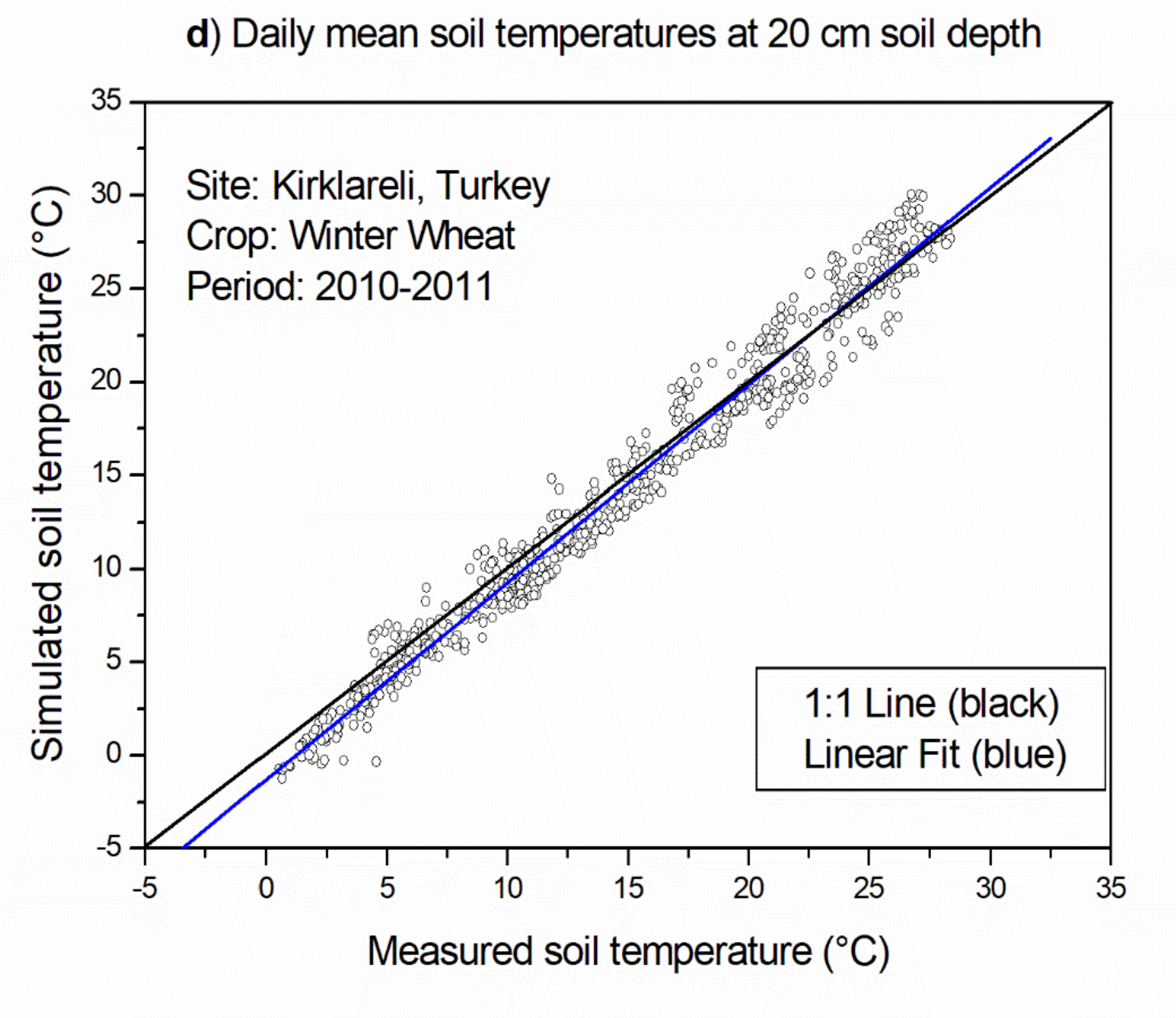
| Kirklareli, Thrace region, Turkey (Validation) | Winter wheat/Bare soil and fallow after winter wheat | Field experiment station | 13.3 °C – 570 mm | Vertisol Cambisol | M | M | M | M |
| Hamme, Belgium (Validation) | Permanent short grass | Field experiment station | 10.6 °C – 852 mm | Eutric Fluvic Gleyic Cambisol | M | M | E | E |
| Purbach East Austria (Validation) | Arable – Vineyard | Field experiment station | 10.4 °C – 758 mm | Chernosem | M | M | S | E |
| Grafendorf Southeast Austria (Calibration of snow cover effect/Validation) | Permanent grassland (3–cut) | Field experiment station | 9.4 °C – 716 mm | Cambisol | M | E/M 6 | M | E |
| Obersiebenbrunn Northeast Austria (Validation) | Natural grassland | 10.3 °C – 516 mm | Chernosem | M | M | S | E | |
| CV (kg ha−1) | vf (Dimensionless) |
|---|---|
| 0 | 0 |
| 2500 | 0.848 |
| 4000 | 0.933 |
| 5000 | 0.965 |
| Parameter | Unit | Calibrated Value | First Estimate (Value Used in Subsequent Simulations) |
|---|---|---|---|
| kcg | W m−2 K−1 | 42.0 | 41.0 |
| β | ha kg−1 | 0.000729 | 0.000663 |
| εf | 1 | 0.95 | 0.95 |
| SNOlimit,1 | mm H2O | 0.3 | 0.4 |
| SNOlimit,2 | mm H2O | 13.8 | 13.8 |
| Location | Surface Conditions | Simulation Period | Available Days | Soil Depth (cm) | R | σo (°C) | σs (°C) | RMSE (°C) | RRMSE (%) | IA (0–1) |
|---|---|---|---|---|---|---|---|---|---|---|
| Groß-Enzersdorf Calibration | 4 × 4 m plot bare soil after seedbed preparation | 1 April–24 May 2012 | 54 | 10 | 0.98 | 4.45 | 4.59 | 0.89 | 6.3 | 0.99 |
| Goggendorf Validation | 4 × 4 m plot bare soil in winter wheat stand since 22 June; soil water content simulated | 22 June–9 December 2016 | 116 | 5 | 0.999 | 8.87 | 8.63 | 1.21 | 8.2 | 0.99 |
| 116 | 10 | 0.999 | 8.79 | 8.31 | 1.17 | 7.9 | 0.99 | |||
| 109 | 20 | 0.99 | 8.07 | 7.75 | 1.01 | 7.2 | 0.99 | |||
| 117 | 40 | 0.999 | 6.73 | 6.66 | 0.59 | 4.1 | 0.99 | |||
| Winter wheat, 15 August harvest –stubble field – 20 September soil mulching– Soil water cont. simulated | 22 June–9 December 2016 | 123 | 5 | 0.999 | 7.47 | 7.55 | 0.69 | 5.2 | 0.99 | |
| 123 | 20 | 0.999 | 6.71 | 6.77 | 0.55 | 4.1 | 0.99 | |||
| 123 | 40 | 0.999 | 5.87 | 5.71 | 0.42 | 3.1 | 0.99 |
| Site Name | Soil Depth | 7–15 MJ m−2 d−1 | >20 MJ m−2 d−1 | ||
|---|---|---|---|---|---|
| cm | n | RMSE (°C) | n | RMSE (°C) | |
| Doksany, CZ | 5 | 1366 | 1.36 | 1207 | 1.88 |
| Kirklareli, TR | 20 | 724 | 1.25 | 560 | 1.71 |
| Hamme, BE | 15 | 1000 | 1.85 | 837 | 2.15 |
| Grafendorf, AT | 10 | 1717 | 1.15 | 1630 | 1.24 |
| Reference Simulation 1 | Reference Conditions | Soil Depth (cm) | Soil Water Content +10 vol % | Soil Water Content −10 vol % | Porosity +10 vol % | Porosity −10 vol % | SBM 2 +1000 kg ha−1 | SBM 2 −1000 kg ha−1 | Sand +55% (Ref: 10%) |
|---|---|---|---|---|---|---|---|---|---|
| Simulation period: 1 January 2016 till 31 December 2016 | Fallow after winter wheat–15 August harvest – straw mulch – 20 September soil mulching | Δ °C—July 2016 mean deviation from reference | |||||||
| 5 | 0.06 | −0.09 | −0.04 | 0.05 | −0.15 | −0.19 | −0.07 | ||
| 10 | 0.05 | −0.09 | 0.00 | 0.02 | −0.15 | −0.17 | −0.17 | ||
| 20 | 0.01 | −0.08 | 0.04 | −0.04 | −0.14 | −0.12 | −0.33 | ||
| 40 | −0.02 | −0.08 | 0.11 | −0.11 | −0.15 | −0.07 | −0.57 | ||
| 60 | −0.03 | −0.09 | 0.13 | −0.14 | −0.18 | −0.04 | −0.75 | ||
| 100 | −0.02 | −0.11 | 0.10 | −0.13 | −0.23 | 0.00 | −0.90 | ||
| Δ °C—October 2016 mean deviation from reference | |||||||||
| 5 | −0.10 | 0.07 | 0.05 | −0.07 | −0.35 | 0.58 | −0.02 | ||
| 10 | −0.08 | 0.06 | 0.01 | −0.03 | −0.34 | 0.57 | 0.10 | ||
| 20 | −0.04 | 0.04 | −0.05 | 0.03 | −0.35 | 0.53 | 0.26 | ||
| 40 | 0.03 | 0.00 | −0.17 | 0.16 | −0.35 | 0.47 | 0.58 | ||
| 60 | 0.08 | −0.02 | −0.27 | 0.26 | −0.33 | 0.41 | 0.91 | ||
| 100 | 0.15 | −0.06 | −0.41 | 0.42 | −0.31 | 0.29 | 1.45 | ||
| Location and Soil Surface | Not Directly Measured Settings/Inputs | Simulation Period | Available Days | Soil Depth (cm) | R | σo (°C) | σs (°C) | RMSE (°C) | RRMSE (%) | IA (0–1) |
|---|---|---|---|---|---|---|---|---|---|---|
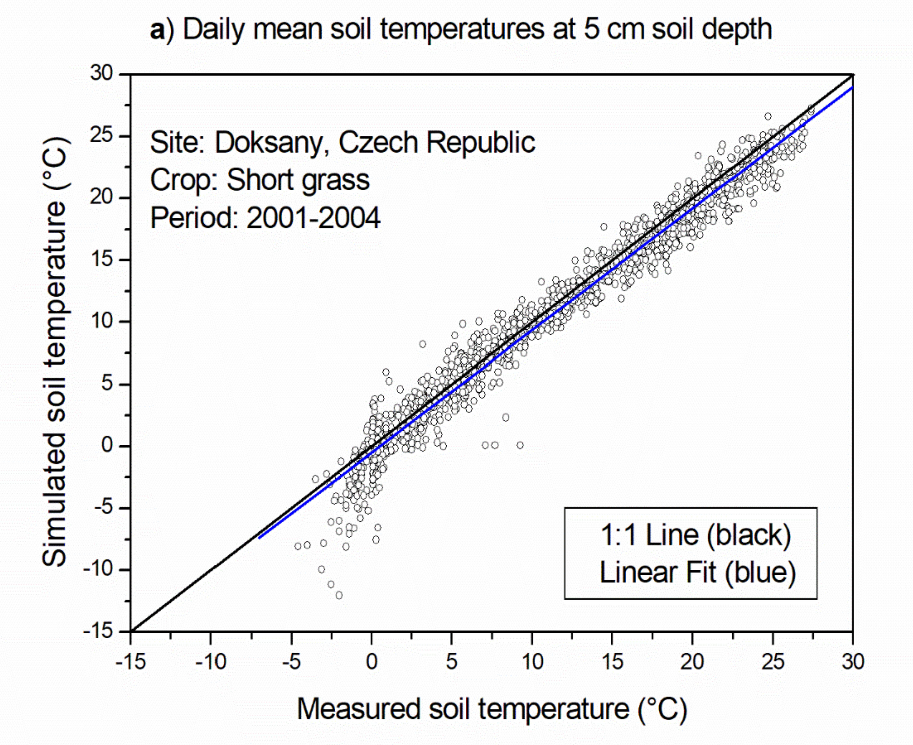
| Doksany – Permanent short grass | Constant surface biomass assumed | Full years 2001–2004 | 1454 | 5 | 0.98 | 8.42 | 8.41 | 1.65 | 15.0 | 0.99 |
| 1454 | 50 | 0.99 | 6.75 | 6.70 | 0.97 | 9.2 | 0.99 | |||
| 1454 | 100 | 0.99 | 5.17 | 5.24 | 0.87 | 8.2 | 0.99 | |||
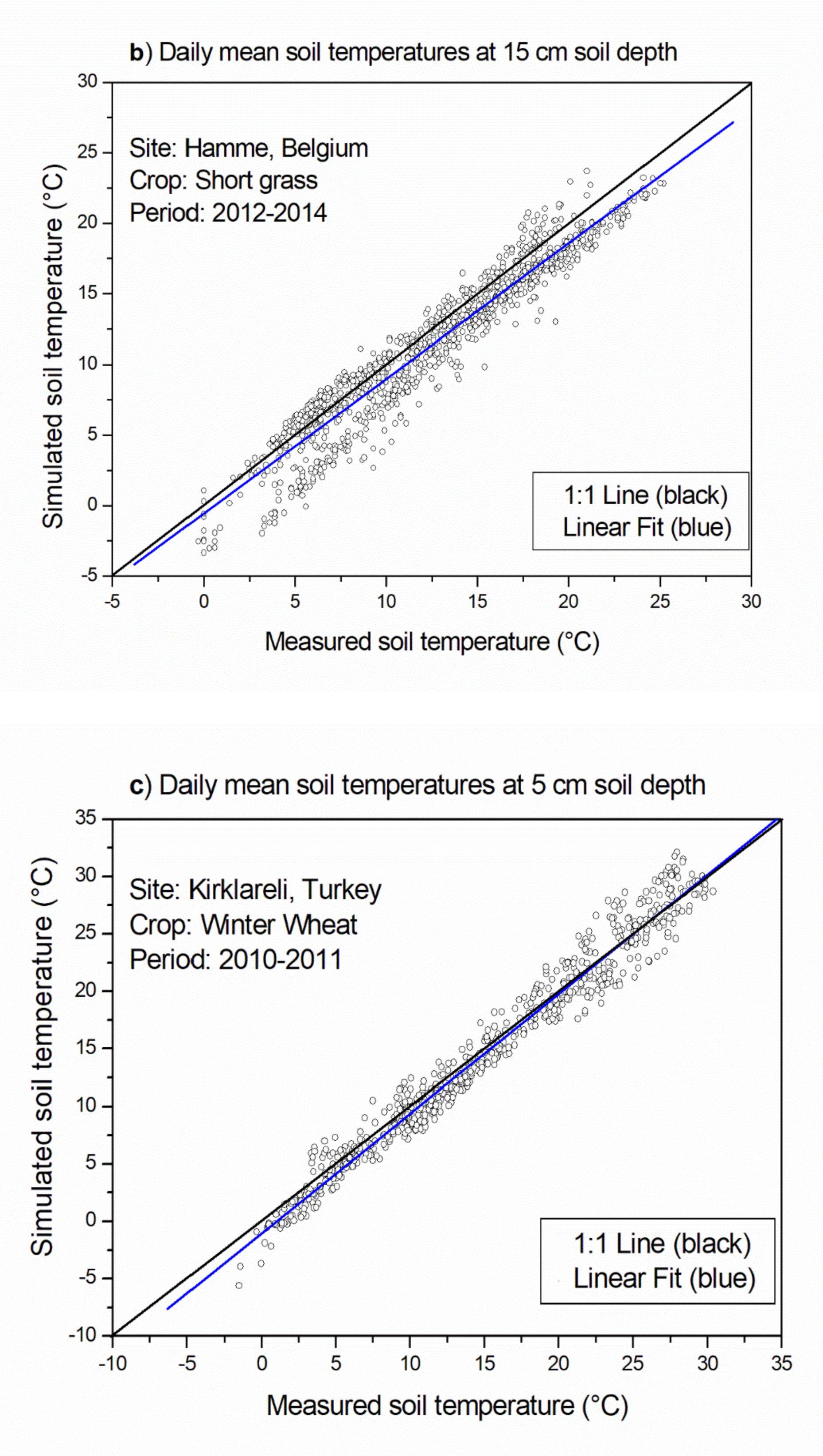
| Kirklareli – Winter wheat/fallow | Constant pore volume assumed | Full years 2010–2011 | 714 | 5 | 0.99 | 8.23 | 8.69 | 1.57 | 10.7 | 0.99 |
| 714 | 20 | 0.99 | 7.57 | 8.11 | 1.45 | 10.0 | 0.99 | |||
| Hamme – Permanent Short grass | Constant soil water content and surface biomass assumed | Full years 2012–2014 | 1096 | 15 | 0.96 | 5.60 | 5.64 | 1.94 | 15.5 | 0.97 |
| Pucking – Cultivated soil on lysimeter | Constant pore volume Crop rotation related surface biomass and soil water content calculated | Sept 1996–Feb 1999 | 745 | 10 | 0.97 | 6.32 | 6.36 | 1.59 | 21.7 | 0.98 |
| 854 | 30 | 0.99 | 6.86 | 6.32 | 1.25 | 14.2 | 0.99 | |||
| Purbach – Cultivated soil under vineyard | Constant pore volume and surface biomass (3000 kg ha−1) Soil water content calculated | July 1999–May 2002 | 941 | 10 | 0.99 | 7.67 | 7.72 | 2.20 | 23.8 | 0.98 |
| 941 | 20 | 0.99 | 7.66 | 7.30 | 1.19 | 11.4 | 0.99 | |||
| 941 | 40 | 0.99 | 7.43 | 6.49 | 1.30 | 12.1 | 0.99 | |||
| 941 | 70 | 0.99 | 7.22 | 5.45 | 2.06 | 19.0 | 0.97 | |||
| Grafendorf – 3–cuts Permanent grassland | Surface biomass calculated according to reported cuts–Snow cover simulated | Years 2004–2007 | 1714 | 10 | 0.98 | 7.11 | 6.98 | 1.45 | 12.9 | 0.99 |
| 1744 | 20 | 0.98 | 6.88 | 6.52 | 1.24 | 11.1 | 0.99 | |||
| 1744 | 30 | 0.99 | 6.59 | 6.09 | 1.13 | 10.2 | 0.99 | |||
| 1739 | 40 | 0.99 | 6.37 | 5.69 | 1.13 | 10.3 | 0.99 | |||
| 1744 | 60 | 0.99 | 5.26 | 5.16 | 0.91 | 8.3 | 0.99 | |||
| Obersieben-brunn – Permanent natural grassland | Constant surface biomass assumed (3000 kg ha−1) Soil water content calculated | Years 2000–2009 | 2557 | 10 | 0.98 | 6.88 | 7.66 | 2.56 | 28.9 | 0.97 |
| 2557 | 50 | 0.99 | 5.80 | 5.23 | 1.11 | 10.2 | 0.99 |
Publisher’s Note: MDPI stays neutral with regard to jurisdictional claims in published maps and institutional affiliations. |
© 2021 by the authors. Licensee MDPI, Basel, Switzerland. This article is an open access article distributed under the terms and conditions of the Creative Commons Attribution (CC BY) license (https://creativecommons.org/licenses/by/4.0/).
Share and Cite
Grabenweger, P.; Lalic, B.; Trnka, M.; Balek, J.; Murer, E.; Krammer, C.; Možný, M.; Gobin, A.; Şaylan, L.; Eitzinger, J. Simulation of Daily Mean Soil Temperatures for Agricultural Land Use Considering Limited Input Data. Atmosphere 2021, 12, 441. https://doi.org/10.3390/atmos12040441
Grabenweger P, Lalic B, Trnka M, Balek J, Murer E, Krammer C, Možný M, Gobin A, Şaylan L, Eitzinger J. Simulation of Daily Mean Soil Temperatures for Agricultural Land Use Considering Limited Input Data. Atmosphere. 2021; 12(4):441. https://doi.org/10.3390/atmos12040441
Chicago/Turabian StyleGrabenweger, Philipp, Branislava Lalic, Miroslav Trnka, Jan Balek, Erwin Murer, Carmen Krammer, Martin Možný, Anne Gobin, Levent Şaylan, and Josef Eitzinger. 2021. "Simulation of Daily Mean Soil Temperatures for Agricultural Land Use Considering Limited Input Data" Atmosphere 12, no. 4: 441. https://doi.org/10.3390/atmos12040441