
Share of Discontinuities in the Ozone Concentration Data from Three Reanalyses

Institute of Atmospheric Physics, Czech Academy of Sciences, 14100 Prague, Czech Republic
*
Authors to whom correspondence should be addressed.
Atmosphere 2021, 12(11), 1508; https://doi.org/10.3390/atmos12111508
Submission received: 8 September 2021
/
Revised: 11 November 2021
/
Accepted: 12 November 2021
/
Published: 16 November 2021
(This article belongs to the Special Issue Discontinuities in Reanalysis Data)
Abstract
:Ozone is a very important trace gas in the stratosphere and, thus, we need to know its time evolution over the globe. However, ground-based measurements are rare, especially in the Southern Hemisphere, and while satellite observations provide broader spatial coverage generally, they are not available everywhere. On the other hand, reanalysis data have regular spatial and temporal structure, which is beneficial for trend analysis, but temporal discontinuities might exist in the data. These discontinuities may influence the results of trend studies. The aim of this paper is to detect discontinuities in ozone data of the following reanalyses: MERRA-2, ERA-5 and JRA-55 with the help of the Pettitt, the Buishand, and the Standard Normal Homogeneity tests above the 500 hPa level. The share of discontinuities varies from 30% to 70% and they are strongly layer dependent. The share of discontinuities is the lowest for JRA-55. Differences between reanalyses were found to be larger than differences between homogeneity tests within one reanalysis. Another aim of this paper is to test the ability of homogeneity tests to detect the discontinuities in 2004 and 2015, when changes in versions of satellite data took place. We showed the discontinuities in 2004 are better detected than those in 2015.
1. Introduction
Ozone is an important trace gas in the atmosphere. Stratospheric ozone protects the biota of the earth from the harmful ultraviolet radiation, while tropospheric ozone is a pollutant and dangerous to human health. At the beginning of the 1970s, ozone research was mostly focused on the connection between the ozone layer and supersonic transport. The great challenge was the discovery of the Antarctic ozone hole. The origin of the ozone hole is in the chemical reactions of anthropogenic halogen radicals, which destroy ozone [1]. As a consequence of these findings, the Montreal Protocol and its amendments were signed, which stopped the production of ozone-depleting substances (ODS). This protocol led to a decrease in ODS concentrations in the stratosphere [2]. There are some signs of the ozone layer’s recovery, especially in the upper stratosphere [3]. In addition, all models predict the future recovery of the ozone layer [4]. The concentration of ODS is not the only factor that has an impact on the ozone layer. Another factor is the cooling of the stratosphere due to the increasing concentration of greenhouse gases in the atmosphere [5] and changes to the Brewer–Dobson circulation influence ozone concentration. Due to the complexities of the factors influencing ozone, proper trend analysis is necessary for an understanding of the ozone layer behaviour. Trend analyses based on ground-based data [6,7] suffer from data being measured at a single location only, and the number of ground-based stations is insufficient, especially in the Southern Hemisphere. Satellite ozone data have broader coverage, and these data are widely used in trend analysis in ozone research [8]. In order to have long data series of satellite ozone measurements, composites from various satellites have been used [9,10,11]. However, it is impossible to measure ozone by satellite under certain conditions and in certain geographical regions (e.g., below dense cloud, polar night). In [12] the critical summary of the current state-of-the-art methods is provided with regards to concerns about trends in the stratospheric ozone. It is also important to note that the usage of the differing measurement techniques can cause the onset of artificial discontinuities in reanalysis data.
On the other hand, the ozone data from reanalyses are temporally and spatially homogeneous, but there is a big question of the suitability of these data for trend analysis due to the possible discontinuities in time series [13]. They can be caused by satellite or instrument replacements or by the assimilation of inhomogeneous basic parameters. For instance, [14] considered the evaluation of trends from reanalyses and found some problems with the homogeneity of this type of data, and [15] searched for the occurrence of discontinuities in MERRA-2 ozone data. The aim of this paper is to extend this analysis to the ERA-5 and JRA-55 data and compare the results from all three reanalyses.
Another aim of this paper is to compare the discontinuity occurrences among selected reanalyses above 500 hPa, with special attention on the artificial discontinuities in series because these make the trend analysis impossible. A further aim is to find the reanalysis with the lowest occurrence of artificial discontinuities. Results will be obtained by several homogeneity tests. We search for the occurrence of discontinuities in reanalyses with the help of the following commonly used homogeneity tests: the Pettitt, the Buishand and the Standard Normal homogeneity tests [16,17,18] for all reanalyses in the period 1980–2017. Detailed explanation of these tests is given in the Supplementary Materials. These tests are general and robust, and they only need continuous data without errors. These conditions are met for reanalysis data. In each grid cell, we search if discontinuities occur or not without distinguishing between natural and artificial discontinuities in the first step. We also explore if the results are test-dependent. This study can help us to compare the data quality in these reanalyses as a first step toward the trend analysis. This paper is divided into the following sections: Section 2 describes the data and method, Section 3 provides results, Section 4 discusses the results and Section 5 contains conclusions.
2. Data and Method
The ozone monthly means from MERRA-2, ERA-5 and JRA-55 above 500 hPa are used for the period 1980–2017. The top modelling level for JRA-55 is 0.1 hPa and for MERRA-2 and ERA-5 is 0.01 hPa. The top available level for all parameters is 1 hPa (JRA-55 and ERA-5) and 0.1 hPa (MERRA-2). Not all available levels are the same for all three reanalysis data sets (see Table 1).
Reanalyses used in this paper cover the whole satellite era. We choose these three reanalyses because they are widely used in atmospheric community and they are the newest at this time.
In MERRA-2, new constraints are applied to ensure the conservation of global dry-air mass and to close the balance between surface water fluxes (precipitation minus evaporation) and changes in total atmospheric water [19]. The modified gravity wave scheme substantially improves the model representation of the quasi biennial oscillation [20,21]. The assimilation of Microwave Limb Sounder (MLS) temperature retrievals at high pressure levels (above 5 hPa) improves the reanalysis at upper levels. The assimilation of MLS stratospheric ozone profiles and Ozone Monitoring Instrument (OMI) column ozone since the beginning of the Aura mission in late 2004 also improve the representation of tropopause [22]. MERRA-2 uses the Three Dimensional Variational (3D VAR) assimilation process and regular latitude–longitude grids from 1000 to 0.01 hPa (1/2° latitude × 5/8° longitude). The warm bias in the upper troposphere has gradually been decreasing because the observing system has been improving.
The changes in observing systems were visible in July 2006, when the GNSS-RO refractivities were included into JRA-55. The impact of changes in observing systems on the JRA-55 time series is reduced compared with JRA-25 but the low-frequency variations are smaller than those of the SSU datasets, especially in the upper stratosphere [23]. Three dimensional daily mean ozone distributions were implemented in JRA-55 for the period after 1979. It was produced separately from the JRA-55 data assimilation system using the T42L68 resolution version of the chemistry climate model (CCM) developed at the Meteorological Research Institute (MRICCM1) [24]. According to [25], the JRA-55 reanalysis well represents the general features of the QBO and SAO. JRA-55 has also reduced biases in the lower stratosphere compared with JRA-25, except in the polar region of the Northern Hemisphere (NH). JRA-55 uses the Four Dimensional Variational (4D VAR) assimilation process and regular latitude–longitude grids from 1000 to 0.1 hPa (0.562° latitude × 0.562° longitude). Detailed description of all reanalyses (including JRA-55 and MERRA-2) can be found in [26,27].
ERA-5 uses 4D-Var data assimilation in CY41R2 of ECMWF’s Integrated Forecast System (IFS), with 137 hybrid sigma/pressure (model) levels in the vertical, with the top level at 0.01 hPa (0.25° latitude × 0.25° longitude). Atmospheric data are available from 37 pressure levels up to 1 hPa. From 2000 to 2006, ERA-5 has a poor fit to radiosonde temperatures in the stratosphere, with a cold bias in the lower stratosphere. In addition, a warm bias higher up persists for much of the period from 1979.
We applied homogeneity tests, the Pettitt, the Buishand and the Standard Normal homogeneity tests [16,17,18], to all reanalyses in the period 1980–2017, to each grid cell separately and independently. In each grid cell, the time series is 38 years long, so tests may be applied to such series and the results can be compared among the tests. Each year was treated separately in each grid cell. The detailed description of the tests used in this paper is given in the Supplementary Materials. The analysis was performed for each grid point; no spatial averaging (longitudinal and latitudinal) was used. Our motivation is to look on data from the point of view of long-term change and trend investigations, which is our main activity in stratospheric research. Spatial averaging is often used in the sense of zonal averaging. However, for example, a longitudinal variation of trends in meridional wind in the middle stratosphere up to the lower mesosphere was observed [28]. This is lost in zonal averaging. On the other hand, temporal averaging in the sense of data used for long-term trend studies does not cause a problem. Monthly averages (used by us) have widely been used in atmospheric trend (and also other) investigations by various authors.
In each grid and each layer, the time series of the ozone concentration is used and the homogeneity tests are applied to look for a discontinuity in them. In each grid, all three tests estimate only one main discontinuity, so this procedure is not able to detect multiple discontinuities. The homogeneity tests used in this paper have been widely used in climatological research, particularly for precipitation and temperature analysis [17,18,29,30,31,32], therefore, we assume their usability also for ozone studies. We are interested primarily in the share of grids with discontinuity to all grids. We must also define the artificial and natural discontinuities. Artificial discontinuities are discontinuities that do not occur in real atmosphere. They arise from changes in the amount of data, version of data, measurement or calibration errors, etc. They influence the trend analysis results and, thus, grid cells with artificial discontinuities cannot be used in trend research without removing THE discontinuities or compensating for them. On the other hand, natural discontinuities are those that are present in real atmosphere and, thus, they must stay in data.
3. Results
First, the share of discontinuities must be defined. The share of discontinuities is the ratio of the number of grids with discontinuities to the number of all grids in certain reanalysis. We can compute the difference in share of discontinuity for each pair of reanalyses for a selected level. This difference is significant when its value is outside the 95% confidence intervals of share of discontinuities. Because we want to compare the results among the tests and among the reanalyses, first we must discuss the statistical significance of differences between them (hereafter, significant always means statistically significant).
A discontinuity may occur for any given grid cell. The discontinuity distribution can be described with a binomial distribution. The distribution mean can be estimated from the test results and the standard deviation is given by
where p is the probability of the event (it is estimated from the test result)
σ = (p(1 − p)/n)0.59
We use the normal approximation for the construction of the confidence interval and, thus, the 95% confidence interval has the width
where p is the probability of the event (in our case the share of discontinuities in a certain layer) and n is the number of grids in a certain layer. The numerator of (2) can be approximated by 1, which overestimates the width of the interval, and n is 207,936, 1,038,240 and 41,760 for MERRA-2, ERA-5 and JRA-55, respectively. After the evaluation of (1), we obtain the overestimated width of confidence intervals: 0.0043, 0.0019 and 0.0096 for MERRA-2, ERA-5 and JRA-55, respectively. The resolution of the share of discontinuities (SD) is about 0.01. Thus, the overestimated width of the confidence interval is lower than the resolution. Therefore, every SD difference is significant due to the large number of grid cells.
1.96 = (p(1 − p)/n)0.5
For each month, each layer and each reanalysis we computed the share of grid cells with discontinuities. Thus, 12 monthly values of the share of discontinuities were obtained for each layer, each reanalysis and each test. From these 12 values we found the minimum, the average and the maximum and constructed the vertical profiles that are displayed in Figure 1 and Figure 2. From these profiles we deduced the range of monthly values of the SD in each layer. We also computed the average value from all values in each vertical profile, as displayed in Table 2 and Table 3. They enable us to compare the SD values among the reanalyses and among the tests.
3.1. Comparison of Share of Discontinuities among Tests within the Same Reanalysis
Figure 1 shows the vertical profile of the average (black), minimal (blue) and maximal (red) share of discontinuities (SD) for MERRA-2 reanalysis obtained by the Pettitt test (upper panel), the Buishand test (middle panel) and the Standard Homogeneity test (lower panel). The SD is clearly layer dependent. The SD is high at 1 hPa, then it decreases down to 7 hPa, where the minimum SD is observed. At lower altitudes its value again increases and reaches another local maximum at 500 hPa. The patterns in the SD vertical profiles are similar for all tests. It is reasonable to compare the values of the SD among tests and on reanalysis, so we computed the average values of the maximal, average and minimal SD, and the results are displayed in Table 2. The highest values of the SD occur for the Standard Homogeneity Normal test, followed by the Buishand test and the smallest SD is observed in the case of the Pettitt test (PT). The differences among tests in the case of the same reanalysis are small.
Supplementary Figure S1 and Table S1 display the vertical profile of SD for ERA-5. There is a tendency of an increasing SD with decreasing height, especially for the Pettitt and the Buishand test, and at about 400 hPa we observed maximum in SD values. The values of the SD are the highest for the Standard test in the case of MERRA-2 and ERA-5.
Results for JRA-55 are displayed on Figure S2 and Table S2. The vertical profile of the SD is similar for all tests with its minimum at 1 hPa and a strong maximum at 450 hPa. There are no differences in the SD between tests.
3.2. Comparison of Share of Discontinuities among Reanalyses within the Same Test
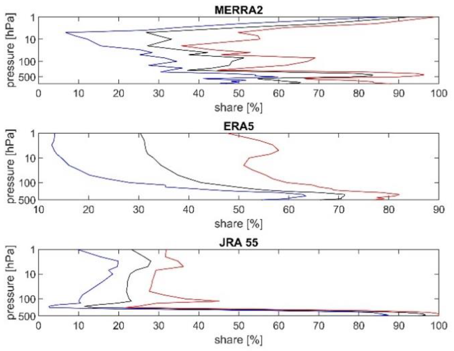
Figure 2 shows the differences between reanalyses in the case of the Pettitt test. There are large differences in the SD between MERRA-2 and ERA-5 below 1 hPa, where the SD for MERRA-2 is much higher than that for ERA-5. The value of the SD in the case of JRA-55 is much lower than those for MERRA-2 and ERA-5. The SD for ERA-5 is a bit lower than that for MERRA-2 (Table 2, Tables S1 and S2).
The profiles of the SD in various reanalyses are shown in Figure S3 for the Buishand test. The values of the SD for JRA-55 are much lower than for the other reanalyses. The SD for ERA-5 is higher than that for MERRA-2.
For the Standard test (Figure S4), again the values of the SD are much lower for JRA-55 and the SD for ERA-5 is higher than for MERRA-2.
3.3. Discontinuities around 2004 and 2015
In the previous sections, the share of discontinuities was investigated without distinguishing between the natural and artificial ones. Now we try to separate them. We know the years in which changes in input data for reanalyses took place and we can look at the share of discontinuities in these years and suppose that these discontinuities are artificial. The following years are regarded as years with changes in output data: 2004 when MERRA-2 and ERA-5 switched from SBUV to MLS, and 2015 when both reanalyses started to use 4.2 MLS data instead of version 2.2 [14]. JRA-55 switched from Nimbus-7 data to OMI in 2004 [23]. Now, we look for the share of discontinuities in the vicinity of these years and we find the year with the maximal share of discontinuities within these periods
The results are presented in Table 3. In this table the share of discontinuities to all discontinuities (not to all grids) is presented for MERRA-2 for the years around 2004 (2003, 2004 and 2005). The maximal values of the SD are seen in 2004 (bold values) for all tests. It means the year 2004 is the year of the main discontinuity. In the case of ERA-5, the situation is more complex. The SD in 2003 and in 2004 (Table S3) are comparable with slightly higher values in 2003. Thus, ERA5 supports the year 2003 as the year of the main discontinuity. JRA-55 has the maximal SD values again in 2004 (Table S4). Therefore, we decided to use the year 2004 as a year with the main discontinuity.
The other period of expected occurrence of discontinuities is the year 2015. Thus, we compute the SD in 2014, 2015 and in 2016, and we look for its maximum. The results are displayed in Table 4. The Pettitt test is not able to capture the discontinuities around 2015 (mathematical zero everywhere). For MERRA-2 and ERA-5 (Table 4 and Table S5) the maximal value of the SD occurs in 2014 for the Buishand and Standard tests but they are very small and, thus, questionable. The Buishand test for JRA-55 gives nearly zero or mathematical zero values everywhere, but the Standard test provides the clear maximum SD value in 2015 (Table S6). Thus, we consider the year 2015 to be the year of the main discontinuity.
3.3.1. Comparison of Share of Discontinuities in 2004 among Tests within the Same Reanalysis
We now compute the share of discontinuities explained by the SD maximum in 2004 to all discontinuities (not all grid cells), similarly as in the case of the share of grids with discontinuities to all grids. The vertical profiles of minima, averages and maxima from all months are displayed them in Figure 3, Figure 4 and Figure 5. The average values from all values in the vertical profile of minima, from all values in the profile of averages, and the same for maxima are shown in Table 5, Table 6 and Table 7, similarly as in the case of the SD from all grids.
The vertical profile of the SD in 2004 to all discontinuities is displayed in Figure 3 for MERRA-2. For all tests, the results are strongly layer and month dependant. There are months in which the explained SD is only several percent (blue line). In the same layer, there are months in which the explained SD is above 70% (red line). The average explained share oscillates from 30% to 50% (Table 5).
The situation for ERA-5 (Figure S5 and Table S7) is different. The SD is not so strongly layer dependent as is the case of MERRA-2, especially in the stratosphere, where we observe an increasing average SD explained by the SD maximum in 2004 with decreasing height. In the troposphere, the SD 2004 is strongly layer dependent with a sharp maximum at 500 hPa. This maximum is seen in all tests. The average SD 2004 is a bit higher in the case of JRA-55 than that of ERA5, but it is below 10% (Table S8).
3.3.2. Comparison of Discontinuity Occurrence in 2004 among Reanalyses within the Same Test
Figure 4 displays vertical profiles of the SD 2004 for the Pettitt test for all reanalyses. The results for the Pettitt test are strongly layer dependent for MERRA-2. The values of the SD 2004 are maximal for MERRA-2, followed by JRA-55 and ERA-5 (Table 5, Tables S7 and S8). In the stratosphere SD 2004 is higher for JRA-55 than for ERA-5.
Similar SD 2004 patterns as regards reanalyses are seen for the Buishand test (Figure S6, Table 5, Tables S7 and S8) and the Standard test (Figure S7, the same tables). We can conclude the patterns of discontinuity occurrence in 2004 are similar for all tests.
3.4. Year 2015
Now, we use the same approach as in the case of year 2004 for the share of discontinuities, which occurred in the year 2015 (SD 2015) to all discontinuities.
3.4.1. Comparison of Share of Discontinuities in 2015 among Tests within the Same Reanalysis
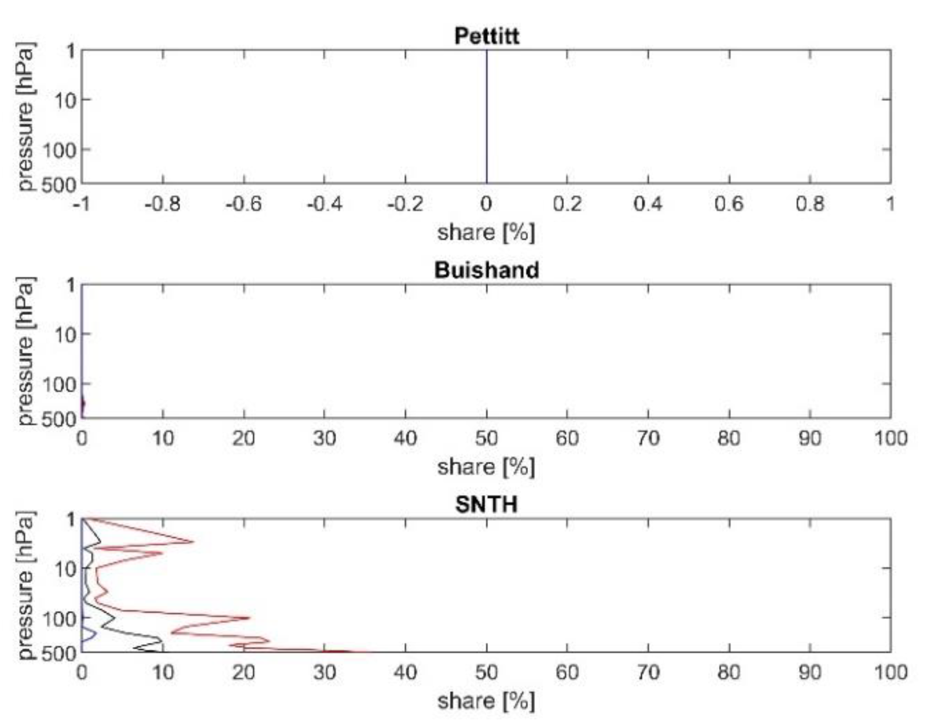
Figure 5 and Table 6 show the vertical profile of SD 2015 for MERRA-2 for all tests used in this paper. We can see the lack of ability of the Pettitt test to catch any discontinuities in 2015 (mathematical zero) because Figure 5 reveals three identical vertical zero lines. The maximal values of SD 2015 for the Buishand test are practically zero, but not mathematical zero. Only the Standard Homogeneity test is able to catch discontinuities in 2015, especially in the troposphere, where SD 2015 may be nearly 40%.
Similar patterns are seen for the SD 2015 in the case of ERA-5. Again the Standard test catches more discontinuities in 2015 than the Buishand test, and we see mathematical zero in the case of the Pettitt test (Figure S8 and Table S9). In the case of JRA-55, we see mathematical zero in the case of the Pettitt test, practically zero for the Buishand test (but not mathematical) and the highest values of the SD 2015 are seen again for the Standard test (Figure S9 and Table S10).
3.4.2. Comparison of Share of Discontinuities in 2015 among Reanalyses within the Same Test
The Pettitt test is not able to detect the change in 2015 (mathematical zero for all reanalyses, Figure not shown, see Table 6, Tables S9 and S10). SD 2015 is zero or nearly zero for all reanalysis (Figure S10).
The Standard test has the best performance in capturing inhomogeneity in 2015. In the case of MERRA-2 (Figure S11 and Table 6, Tables S9 and S10) and JRA-55, an increasing tendency of SD 2015 occurs with decreasing height with maximal values in the troposphere. In the case of ERA-5, the tendency is opposite with maximal SD 2015 in the stratosphere.
3.5. Share of Discontinuities Explained by Changes in 2004 and 2015
Now we deal with the total share of discontinuities explained by the changes in 2004 and 2015 (SDE) to all discontinuities. In these two years we see the reason for the discontinuity occurrence. The reason for the existence of the rest of the discontinuities is unknown, we can only speculate.
3.5.1. Comparison of Share of Explained Discontinuities (SDE) among Tests within the Same Reanalysis
The SDE in the case of MERRA-2 is strongly layer dependent (Figure 6 and Table 7) More than 50% of discontinuities are explained on average by the changes in 2004 and 2015, and at some layers this share is above 80%.
In the case of ERA5, the layer dependence is weaker, especially in the stratosphere (Figure S12 and Table S11), but the share of explained discontinuity is much lower (5–10%).
In the case of JRA-55, the maximal values of the SDE are observed in the stratosphere (Figure S13 and Table S12) and the share is the lowest (about 5%).
Thus, more than 50% of all discontinuities are explained by two years with known discontinuities, 2004 and 2015, for MERRA2. For ERA-5 and JRA-55, the results are worse.
3.5.2. Comparison of Share of Explained Discontinuities among Reanalyses within the Same Test
The maximal value of the SDE is observed for MERRA-2, this value is lower for ERA-5 and JRA-55 for the Pettit test (Figure 7 and Table 7, Tables S11 and S12).
Similar patterns are seen for the Standard test (Figure S14, Table 7, Tables S11 and S12) and for the Buishand (Figure S15 and Table 7, Tables S11 and S12 Overall the SDE is smallest for ERA-5.
4. Discussion
4.1. MERRA-2
The share of discontinuities is from 35% to 70% with the average above 50%. The vertical profile of the SD exhibits a maximum below 1 hPa, then it declines to the minimum at 7 hPa, and then it increases to a maximum at about 450 hPa. These results are confirmed by all tests of homogeneity. The explained share of discontinuity is strongly layer dependant and it oscillates from 35% to 70%, which means that this amount of discontinuities can be explained by the SD in 2004 and 2015. The change in 2004 is much better captured than the change in 2015. This is valid for all reanalyses. According to our opinion, this is because the year 2015 is near the end of the time series (in 2017). We can create the following artificial series: 9,11,9,11,9,11,9,11,9,11,29,31,29,31,29,31,29,31,29,31. There is a discontinuity at the 11th member. The position of discontinuity will be gradually shifted to the end of the series. The performance of the homogeneity tests is displayed in Table 8. Numbers in black mean the test properly indicates the position of discontinuity and the discontinuity is significant. Numbers in red mean there is a problem in discontinuity detection (position or significance). On the first row there is a number of the series’ members in which the discontinuity occurs. The results from all homogeneity tests are shown in this table. Until the 14th member all tests are able to capture the position of discontinuity well, and the test is successful in catching the position of discontinuity (it gives the 14th member, but the discontinuity is present at the 15th member). However, according to this test, this discontinuity is significant, so the results of this test are wrong (wrong detection of position or insignificant discontinuity is printed in red in Table 8). From the 16th member to the 19th member, all discontinuities are regarded as insignificant, so the Pettitt test is not able to catch properly the discontinuities from the 15th member. This result explains the lack of ability of the Pettitt test to capture the discontinuities in 2015. The Buishand test gives the position of discontinuity properly to the 18th member. It gives insignificant discontinuity at the 19th member (the last possible position of discontinuity). This test also gives better results than the Pettitt test in capturing the 2015 discontinuity. The Standard Homogeneity test is the only test that is also able to catch the discontinuity at the 19th member. This discontinuity is also significant and this explains the best performance of this test in capturing the 2015 discontinuities. A detailed explanation of tests used in this paper, with examples, is in the Supplementary Materials. The values of the test statistics are the highest when the discontinuity is situated in the middle of series. Their values decrease when the discontinuity is shifted to both ends of the series and, thus, in these cases it may be detected as insignificant.
4.2. ERA-5
In this reanalysis, the SD is similar to that in MERRA-2, but the vertical profile of the SD is different, especially at 1 hPa, where we observe the minimum value of the SD, then the values of the SD increase to the tropospheric maxima. This vertical profile is confirmed by all homogeneity tests. The explained share of discontinuity is less layer dependent than that of MERRA-2, especially in the stratosphere, and the values of SDE are lower than in the case of MERRA-2 (from 5% to 45%).
4.3. JRA-55
The vertical profiles of the SD are similar to that of ERA5, but the SD values are the smallest from all three reanalyses, according to all homogeneity tests (from 25% to 50%). The vertical profile of the SDE is again similar to that of ERA-5, but their values are a bit higher, i.e., more of the SD is explained by years 2004 and 2015.
4.4. Pettitt Test
The values of the SD from the Pettitt test are similar to those of Buishand and a bit lower than from the Standard Homogeneity test. This is true for MERRA-2 and ERA-5 but not for JRA-55. For JRA-55, the maximal values of the SD are seen for the Buishand test. The Pettitt test is not able to catch the change in 2015 at all (mathematical zero).
4.5. Buishand Test
The Buishand test does not capture the 2015 change well; the value of the SD 2015 is nearly zero (but not mathematical zero). The SDE is similar to that from the Pettitt test. All tests have much better performance in capturing the SD occurrence in 2004 than in 2015 due to the vicinity of the time series end in 2017. Only the Standard Homogeneity test, to some extent, succeeded in the detection of the 2015 change.
4.6. The Standard Normal Homogeneity Test
The share of discontinuities is higher for this test than the other tests for MERRA-2 and ERA-5. The share explained by the change in 2004 is lower than that from the Pettitt and the Buishand test. On the other hand, this test is the only test that is able to capture the SDs in 2015. It is the reason for which the explained share is the highest for this test in the case of MERRA-2 and ERA-5 reanalyses. In the case of JRA-55, the SD is similar to the other tests.
Each test used in this paper may be used for the detection of discontinuities in ozone concentration data from reanalyses data. The performance of the tests decreases toward the end of series, but the performance of the Standard Homogeneity test is the best.
We must say a few words to the occurrence of discontinuities in the time series. Not all discontinuities are wrong, only the artificial ones. Real/natural discontinuities must remain in the time series. We found that the minority of discontinuities can be explained by the change in 2004 and in 2015. The rest of the discontinuities are unexplained. There may be various natural sources of discontinuities in the time series, for example, volcanic eruptions or sudden cooling of the tropical tropopause resulting in a drop in lower stratospheric water vapour (in 2001). The detailed analysis of the unexplained discontinuities should be a matter for a future paper.
What could be the impact of the results of this paper on future ozone trend analyses? If one wants to explore reanalyses data for trend analyses, it is necessary to look at the correlation between the trend patterns and patterns of discontinuity occurrence. If the correlations are present, the discontinuity influence must be taken into account.
5. Conclusions
A statistical analysis of the share of discontinuities has been performed for three modern reanalyses, MERRA-2, ERA5 and JRA-55, using three different tests of homogeneity, namely the Pettitt, Buishand and Standard Normal Homogeneity tests. The main results of this paper are as follows:
- Differences among reanalyses are larger than the differences among homogeneity tests within one reanalysis.
- The share of discontinuities oscillates from 30% to 70% and it is the lowest for JRA-55.
- The minority of discontinuities can be explained by the occurrence of discontinuities in 2004 and in 2015.
- The Pettitt and the Buishand test are not able to capture the change in 2015.
- Only the Standard Homogeneity test can catch the 2015 change.
These results should be considered when the ozone data from reanalyses are used for long-term trend studies.
Supplementary Materials
The following are available online at https://www.mdpi.com/article/10.3390/atmos12111508/s1, Figure S1: Vertical profile of average (black), minimal (blue) and maximal (red) share of discontinuities to all grids from all months from ERA-5 for the Pettitt test (upper panel), the Buishand test (middle panel), and the Standard Normal Ho-mogeneity test (SNTH, lower panel), Figure S2: The same as Figure S1, but for JRA-55, Figure S3: Vertical profile of average (black), minimal (blue) and maximal (red) share of discontinuities to all grids from all months from the Buishand test for MERRA-2 (upper panel), ERA-5 (middle panel), and JRA-55 (lower panel), Figure S4: The same as Figure S3, but for the Standard homogeneity test, Figure S5: Vertical profile of average (black), minimal (blue) and maximal (red) share of explained discontinuities by the change in 2004 to all discontinuities from all months from ERA-5 for the Pettitt test (upper panel), the Buishand test (middle panel), and the Standard Normal Homogeneity test (lower panel), Figure S6: The same as Figure S5, but for JRA-55, Figure S7: Vertical profile of average (black), minimal (blue) and maximal (red) share of explained discontinuities by the change in 2004 to all grids from all months from the Buishand test for MERRA-2 (upper panel), ERA-5 (middle panel), and JRA-55 (lower panel), Figure S8: The same as Figure S7, but for the Standard homogeneity test, Figure S9: Vertical profile of average (black), minimal (blue) and maximal (red) share of explained discontinuities by the change in 2015 to all discontinuities from all months from ERA-5 for the Pettitt test (upper panel), the Buishand test (middle panel), and the Stand-ard Normal Homogeneity test (SNTH, lower panel), Figure S10: The same as Figure S9, but for JRA-55, Figure S11: Vertical profile of average (black), minimal (blue) and maximal (red) share of explained discontinuities by the change in 2015 to all grids from all months from the Buishand test for MERRA-2 (upper panel), ERA-5 (middle panel), and JRA-55 (lower panel), Figure S12: The same as Figure S11, but for the Standard homogeneity test, Figure S13: Vertical profile of average (black), minimal (blue) and maximal (red) share of explained discontinuities by the change in 2004 and in 2015 to all discontinuities from all months from ERA-5 for the Pettitt test (upper panel), the Buishand test (middle panel), and the Standard Normal Homogeneity test (SNTH, lower panel, Figure S14: The same as Figure S13, but for JRA-55, Figure S15: The same as Figure S15, but for the Standard homogeneity test, Table S1: Minimal, average, and maximal share of discontinuities in percentage to all grids from all months from ERA-5 for the Pettitt test, the Buishand test, and the Standard Normal Homogeneity test, Table S2: The same as Table S1, but for JRA-55, Table S3: Minimal, average and maximal share of discontinuities in percentage to all discontinuities in 2003/2004/2005 from ERA-5 for the Pettitt test, the Buishand test and the Standard Normal Homogeneity test, Table S4: The same as Table S3, but for JRA-55, Table S5: Minimal, average and maximal share of discontinuities in percentage to all discontinuities in 2014/2015/2016 from ERA-5 for the Pettitt test, the Buishand test and the Standard Normal Homogeneity test, Table S6: The same as Table S5, but for JRA-55, Table S7: Minimal, average, and maximal share of explained discontinuities in percentage by the change in 2004 to all discontinuities from all months from ERA-5 for the Pettitt test, the Buishand test, and the Standard Normal Homogeneity test, Table S8: The same as Table S7, but for JRA-55, Table S9: Minimal, average, and maximal share in percentage of explained discontinuities by the change in 2015 to all discontinuities from all months from ERA-5 for the Pettitt test, the Buishand test, and the Standard Normal Homogeneity test. 0 means mathematical zero, 0.0 nearly zero, but not mathematical zero, Table S10: The same as Table S5, but for JRA-55, Table S11: Minimal, average, and maximal share of explained discontinuities in percentage by the change in 2004 and in 2015 to all discontinuities from all months from ERA-5 for the Pettitt test, the Buishand test, and the Standard Normal Homogeneity test, Table S12: The same as Table S6, but for JRA-55, Table S13: Values of series (second row), cumulative sum of deviations from mean divided by standard deviations (third row) and the absolute maximal values of test statistic (fourth row), Table S14: Threshold values of statistic for the Buishand test for various significance level and various length of time series, Table S15: Values of series (second row), Ut, T statistic (third row) and KT (fourth row), Table S16: Values of series (second row), Tk statistic (third row) and maximal value of Tk when we shift with the discontinuity (fourth row), Table S17: Threshold values of statistic for the Standard homogeneity test for various significance level and various length of time series.
Author Contributions
This paper was prepared in close collaboration with all authors but a major part of the work was completed by P.K.; conceptualization P.K.; investigation, M.K. and J.L.; software, R.L. All authors have read and agreed to the published version of the manuscript.
Funding
Support by the Czech Science Foundation via Grant 21-03295S is acknowledged. We also thank LISA-Lidar measurements for identifying streamers and analysing atmospheric waves, AEOLUS-INNOVATION, Contract No. 4000133567/20/I-BG.
Institutional Review Board Statement
Not applicable.
Informed Consent Statement
Not Applicable.
Data Availability Statement
ERA-5:https://cds.climate.copernicus.eu/cdsapp#!/home (accessed on 8 November 2021); JRA-55: https://rda.ucar.edu/datasets/ds628.0/#access (accessed on 8 November 2021); MERRA-2: https://cmr8.earthdata.nasa.gov/search/concepts/C1276812931-GES_DISC.html (accessed on 8 November 2021).
Conflicts of Interest
The authors declare no conflict of interest.
References
- Solomon, S. Stratospheric ozone depletion: A review of concepts and history. Rev. Geophys. 1999, 37, 275–316. [Google Scholar] [CrossRef]
- World Meteorological Organization. Monitoring Project Report; World Meteorological Organization: Geneva, Switzerland, 2014; p. 416. [Google Scholar]
- Harris, N.R.P.; Hassler, B.; Tummon, F.; Bodeker, G.E.; Hubert, D.; Petropavlovskikh, I.; Steinbrecht, W.; Anderson, J.; Bhartia, P.K.; Boone, C.D.; et al. Past changes in the vertical distribution of ozone—Part 3: Analysis and interpretation of trends. Atmos. Chem. Phys. 2015, 15, 9965–9982. [Google Scholar] [CrossRef] [Green Version]
- Eyring, V.; Cionni, I.; Bodeker, G.E.; Charlton-Perez, A.J.; Kinnison, D.E.; Scinocca, J.F.; Waugh, D.W.; Akiyoshi, H.; Bekki, S.; Chipperfield, M.P.; et al. Multi-model assessment of stratospheric ozone return dates and ozone recovery in CCMVal-2 models. Atmos. Chem. Phys. 2010, 10, 9451–9472. [Google Scholar] [CrossRef] [Green Version]
- Waugh, D.W.; Oman, L.; Kawa, S.R.; Stolarski, R.S.; Pawson, S.; Douglass, A.R.; Newman, P.A.; Nielsen, J.E. Impacts of climate change on stratospheric ozone recovery. Geophys. Res. Lett. 2009, 36, L03805. [Google Scholar] [CrossRef] [Green Version]
- McLandress, C.H.; Sheepherd, T.G. Simulated anthropogenic changes in the brewer-dobson circulation, including its extension to high latitudes. J. Clim. 2009, 22, 1516–1540. [Google Scholar] [CrossRef]
- Krzyscin, J.W.; Borkowski, J.L. Variabilty of the total ozone trend over Europe for the period 1950–2004 derived from reconstructed data. Atmos. Chem. Phys. 2008, 8, 2847–2857. [Google Scholar] [CrossRef] [Green Version]
- Jones, A.; Urban, J.; Murtagh, D.P.; Eriksson, P.; Brohede, S.; Haley, C.; Degenstein, D.; Bourassa, A.; von Savigny, C.; Sonkaew, T.; et al. Evolution of stratospheric ozone and water vapour time series studied with satellite measurements. Atmos. Chem. Phys. 2009, 9, 6055–6075. [Google Scholar] [CrossRef] [Green Version]
- Ball, W.T.; Alsing, J.; Staehelin, J.; Davis, S.M.; Froidevaux, L.; Peter, T. Stratospheric ozone trends for 1985–2018: Sensitivity to recent large variability. Atmos. Chem. Phys. 2019, 19, 12731–12748. [Google Scholar] [CrossRef] [Green Version]
- Bourassa, A.E.; Degenstein, D.A.; Randel, W.J.; Zawodny, J.M.; Kyrölä, E.; McLinden, C.A.; Sioris, C.E.; Roth, C.Z. Trends in stratospheric ozone derived from merged SAGE II and Odin-OSIRIS satellite observations. Atmos. Chem. Phys. 2014, 14, 6983–6994. [Google Scholar] [CrossRef] [Green Version]
- Tummon, F.; Hassler, B.; Harris, N.R.P.; Staehelin, J.; Steinbrecht, W.; Anderson, J.; Bodeker, J.E.; Bourassa, A.; Davis, S.M.; Degenstein, D.; et al. Intercomparison of vertically resolved merged satellite ozone data sets: Interannual variability and long-term trends. Atmos. Chem. Phys. 2014, 14, 25687–25745. [Google Scholar] [CrossRef] [Green Version]
- Stratosphere-Troposphere Processes and their Role in Climate (SPARC). SPARC Report N°9 (2019) of The SPARC LOTUS Activity: SPARC/IO3C/GAW Report on Long-term Ozone Trends and Uncertainties in the Stratosphere; Petropavlovskikh, I., Godin-Beekmann, S., Hubert, D., Damadeo, R., Hassler, B., Sofieva, V., Eds.; SPARC Office: Oberpfaffenhofen, Germany, 2019. [Google Scholar] [CrossRef]
- Bengtsson, L.; Hagemann, S.; Hodges, K.I. Can climate trends be calculated from reanalysis data? J. Geophys. Res. Atmos. 2004, 109, D11111. [Google Scholar] [CrossRef] [Green Version]
- Shangguan, M.; Wang, W.; Jin, S. Variability of temperature and ozone in the upper troposphere and lower stratosphere from multi-satellite observations and reanalysis data. Atmos. Chem. Phys. 2019, 19, 6659–6679. [Google Scholar] [CrossRef] [Green Version]
- Križan, P.; Kozubek, M.; Laštovička, J. Discontinuities in the ozone concentration time series from MERRA-2 reanalysis. Atmosphere 2019, 10, 812. [Google Scholar] [CrossRef] [Green Version]
- Pettitt, A.N. A non-parametric approach to the change point detection. Appl. Stat. 1979, 28, 126–135. [Google Scholar] [CrossRef]
- Buishand, T.A. Some Methods for Testing the Homogeneity of Rainfall Records. J. Hydrol. 1982, 58, 11–27. [Google Scholar] [CrossRef]
- Alexandersson, H. A homogeneity test applied to precipitation data. J. Climatol. 1986, 6, 661–675. [Google Scholar] [CrossRef]
- Takacs, L.L.; Suárez, M.J.; Todling, R. Maintaining atmospheric mass and water balance in reanalyses. Q. J. R. Meteorol. Soc. 2016, 142, 1565–1573. [Google Scholar] [CrossRef] [Green Version]
- Molod, A.; Takacs, L.; Suarez, M.; Bacmeister, J. Development of the GEOS-5 atmospheric general circulation model: Evolution from MERRA to MERRA-2. Geosci. Model Dev. 2015, 8, 1339–1356. [Google Scholar] [CrossRef] [Green Version]
- Coy, L.; Wargan, K.; Molod, A.M.; McCarty, W.R.; Pawson, S. Structure and dynamics of the quasi-biennial oscillation in MERRA-2. J. Clim. 2016, 29, 5339–5354. [Google Scholar] [CrossRef]
- Randles, C.A.; da Silva, A.M.; Buchard, V.; Darmenov, A.; Colarco, P.R.; Aquila, V.; Bian, H.; Nowottnick, E.P.; Pan, X.; Smirnov, A.; et al. The MERRA-2 Aerosol Assimilation, NASA Technical Report Series on Global Modeling and Data Assimilation; NASA/TM-2016-104606; NASA Goddard Space Flight Center: Greenbelt, MD, USA, 2016; Volume 45.
- Kobayashi, S.; Ota, Y.; Harada, Y.; Ebita, A.; Moriya, M.; Onoda, H.; Onogi, K.; Kamahori, H.; Kobayashi, C.; Endo, H.; et al. The JRA-55Reanalysis: General Specifications and Basic Characteristics. J. Meteor. Soc. Jpn. 2015, 93, 5–48. [Google Scholar] [CrossRef] [Green Version]
- Shibata, K.; Deushi, M.; Sekiyama, T.T.; Yoshimura, H. Development of an MRI chemical transport model for the study of stratospheric chemistry. Pap. Geophys. Meteor. 2005, 55, 75–119. [Google Scholar] [CrossRef] [Green Version]
- Harada, Y.; Kamahori, H.; Kobayashi, C.; Endo, H.; Kobayashi, S.; Ota, Y.; Onoda, H.; Onogi, K.; Miyaoka, K.; Takahashi, K. The JRA-55 Reanalysis: Representation of atmospheric circulation and climate variability. J. Meteor. Soc. Jpn. 2016, 94, 269–302. [Google Scholar] [CrossRef] [Green Version]
- Fujiwara, M.; Wright, J.S.; Manney, G.L.; Gray, L.J.; Anstey, J.; Birner, T.; Davis, S.; Gerber, E.P.; Harvey, V.L.; Hegglin, M.I.; et al. Introduction to the SPARC Reanalysis Intercomparison Project (S-RIP) and overview of the reanalysis systems. Atmos. Chem. Phys. 2017, 17, 1417–1452. [Google Scholar] [CrossRef] [Green Version]
- Gelaro, R.W.; McCarty, M.J.; Suárez, R.; Todling, A.; Molod, L.; Takacs, C.A.; Randles, A.; Darmenov, M.G.; Bosilovich, R.; Reichle, K.; et al. The modern-era retrospective analysis for research and applications, Version 2 (MERRA-2). J. Clim. 2017, 30, 5419–5454. [Google Scholar] [CrossRef]
- Kozubek, M.; Krizan, P.; Lastovicka, J. Northern Hemisphere stratospheric winds in higher midlatitudes: Longitudinal distribution and long-term trends. Atmos. Chem. Phys. 2015, 15, 2203–2213. [Google Scholar] [CrossRef] [Green Version]
- Javari, M. Trend and homogeneity analysis of precipitation in Iran. Climate 2016, 4, 44. [Google Scholar] [CrossRef]
- Firat, M.; Dikbas, F.; Cem Koç, A.; Gungor, M. Missing data analysis and homogeneity test for Turkish precipitation series. Sadhana 2010, 35, 707–720. [Google Scholar] [CrossRef]
- Wijngaard, J.B.; Kleink Tank, A.M.G.; Konnen, G.P. Homogeneity of 20th century European daily temperature and precipitation series. Int. J. Climatol. 2003, 23, 679–692. [Google Scholar] [CrossRef]
- Kozubek, M.; Krizan, P.; Lastovicka, J. Homogeneity of the temperature data series fromERA-5 and MERRA-2 and temperature trends. Atmosphere 2020, 11, 235. [Google Scholar] [CrossRef] [Green Version]
Figure 1.
Vertical profile of average (black), minimal (blue) and maximal (red) share of discontinuities to all grids from all months from MERRA-2 for the Pettitt test (upper panel), the Buishand test (middle panel) and the Standard Normal Homogeneity test (SNTH, lower panel).
Figure 1.
Vertical profile of average (black), minimal (blue) and maximal (red) share of discontinuities to all grids from all months from MERRA-2 for the Pettitt test (upper panel), the Buishand test (middle panel) and the Standard Normal Homogeneity test (SNTH, lower panel).

Figure 2.
Vertical profile of average (black), minimal (blue) and maximal (red) share of discontinuities to all grids from all months from the Pettitt test for MERRA-2 (upper panel), ERA-5 (middle panel), and JRA-55 (lower panel).
Figure 2.
Vertical profile of average (black), minimal (blue) and maximal (red) share of discontinuities to all grids from all months from the Pettitt test for MERRA-2 (upper panel), ERA-5 (middle panel), and JRA-55 (lower panel).

Figure 3.
Vertical profile of average (black), minimal (blue) and maximal (red) share of explained discontinuities by the change in 2004 to all discontinuities from all months in the period 1980–2017 from MERRA-2 for the Pettitt test (upper panel), the Buishand test (middle panel) and the Standard Normal Homogeneity test (SNTH, lower panel).

Figure 4.
Vertical profile of average (black), minimal (blue) and maximal (red) share of explained discontinuities by the year 2004 to all grids from all months from the Pettitt test for MERRA-2 (upper panel), ERA-5 (middle panel) and JRA-55 (lower panel).
Figure 4.
Vertical profile of average (black), minimal (blue) and maximal (red) share of explained discontinuities by the year 2004 to all grids from all months from the Pettitt test for MERRA-2 (upper panel), ERA-5 (middle panel) and JRA-55 (lower panel).

Figure 5.
Vertical profile of average (black), minimal (blue) and maximal (red) share of explained discontinuities by the change in 2015 to all discontinuities from all months from MERRA-2 for the Pettitt test (upper panel), the Buishand test (middle panel) and the Standard Normal Homogeneity test (SNTH, lower panel).

Figure 6.
Vertical profile of average (black), minimal (blue) and maximal (red) share of explained discontinuities by the change in 2004 and 2015 to all discontinuities from all months from MERRA-2 for the Pettitt test (upper panel), the Buishand test (middle panel) and the Standard Normal Homogeneity test (SNTH, lower panel).

Figure 7.
Vertical profile of average (black), minimal (blue) and maximal (red) share of explained discontinuities by the change in 2004 and 2015 to all grids from all months from the Pettitt test for MERRA-2 (upper panel), ERA-5 (middle panel) and JRA-55 (lower panel).
Figure 7.
Vertical profile of average (black), minimal (blue) and maximal (red) share of explained discontinuities by the change in 2004 and 2015 to all grids from all months from the Pettitt test for MERRA-2 (upper panel), ERA-5 (middle panel) and JRA-55 (lower panel).


Table 1.
Layers in reanalyses used in this paper.
| hPa | 0.1 | 0.3 | 0.4 | 0.5 | 0.7 | 1 | 2 | 3 | 4 | 5 | 7 | 10 | 20 | 30 | 40 | 50 | 70 | 100 | 125 | 150 | 175 | 200 | 225 | 250 | 300 | 350 | 400 | 450 | 500 |
|---|---|---|---|---|---|---|---|---|---|---|---|---|---|---|---|---|---|---|---|---|---|---|---|---|---|---|---|---|---|
| MERRA-2 | * | * | * | * | * | * | * | * | * | * | * | * | * | * | * | * | * | * | * | * | * | * | * | * | * | * | |||
| ERA-5 | * | * | * | * | * | * | * | * | * | * | * | * | * | * | * | * | * | * | * | * | * | * | |||||||
| JRA-55 | * | * | * | * | * | * | * | * | * | * | * | * | * | * | * | * | * | * | * | * | * |
Table 2.
Minimal, average and maximal share of discontinuities to all grids in percentage from all months from MERRA-2 for the Pettitt test, the Buishand test and the Standard Normal Homogeneity test.
Table 2.
Minimal, average and maximal share of discontinuities to all grids in percentage from all months from MERRA-2 for the Pettitt test, the Buishand test and the Standard Normal Homogeneity test.
| MERRA-2 | Pettitt | Buishand | Standard |
|---|---|---|---|
| minimum | 35.4 | 36.9 | 41.9 |
| average | 52.6 | 54.6 | 60.0 |
| maximum | 66.4 | 69.7 | 72.6 |
Table 3.
Minimal, average and maximal share of discontinuities to all discontinuities in percentage in 2003/2004/2005 from MERRA-2 for the Pettitt test, the Buishand test and the Standard Normal Homogeneity test.
Table 3.
Minimal, average and maximal share of discontinuities to all discontinuities in percentage in 2003/2004/2005 from MERRA-2 for the Pettitt test, the Buishand test and the Standard Normal Homogeneity test.
| MERRA-2 | Pettitt | Buishand | SNTH |
|---|---|---|---|
| minimum | 3.8/1.2/0.2 | 1.7/1.9/0.4 | 0.6/1.7/0.4 |
| average | 17.3/32.7/2.5 | 15.9/34.0/3.4 | 12.1/29.7/4.1 |
| maximum | 53.9/59.1/7.5 | 56.0/61.4/9.5 | 48.4/56.4/11.3 |
Table 4.
The same as Table 3, but for 2014/2015/2016.
Table 4.
The same as Table 3, but for 2014/2015/2016.
| MERRA-2 | Pettitt | Buishand | SNTH |
|---|---|---|---|
| minimum | 0/0/0 | 0/0/0 | 0.2/0.1/0.0 |
| average | 0/0/0 | /0.0/0 | 4.6/4.1/0.7 |
| maximum | 0/0/0 | 0.3/0.1/0 | 12.4/13.0/3.1 |
Table 5.
Minimal, average, and maximal share of explained discontinuities in percentage by the change in 2004 to all discontinuities from all months from MERRA-2 for the Pettitt test, the Buishand test and the Standard Normal Homogeneity test.
Table 5.
Minimal, average, and maximal share of explained discontinuities in percentage by the change in 2004 to all discontinuities from all months from MERRA-2 for the Pettitt test, the Buishand test and the Standard Normal Homogeneity test.
| MERRA-2 | Pettitt | Buishand | Standard |
|---|---|---|---|
| minimum | 1.2 | 1.9 | 1.7 |
| average | 32.7 | 34.0 | 29.8 |
| maximum | 59.1 | 61.4 | 56.4 |
Table 6.
Minimal, average and maximal share of explained discontinuities in percentage by the change in 2015 to all discontinuities from all months from MERRA-2 for the Pettitt test, the Buishand test and the Standard Normal Homogeneity test. Here, 0 means mathematical zero, 0.0 nearly zero but not mathematical zero.
| MERRA-2 | Pettitt | Buishand | Standard |
|---|---|---|---|
| minimum | 0 | 0 | 0.1 |
| average | 0 | 0.0 | 4.1 |
| maximum | 0 | 0.1 | 13.0 |
Table 7.
Minimal, average and maximal share of explained discontinuities in percentage by the change in 2004 and in 2015 to all discontinuities from all months from MERRA-2 for the Pettitt test, the Buishand test and the Standard Normal Homogeneity test.
Table 7.
Minimal, average and maximal share of explained discontinuities in percentage by the change in 2004 and in 2015 to all discontinuities from all months from MERRA-2 for the Pettitt test, the Buishand test and the Standard Normal Homogeneity test.
| MERRA-2 | Pettitt | Buishand | Standard |
|---|---|---|---|
| minimum | 1.2 | 1.9 | 3.0 |
| average | 32.7 | 34.0 | 33.8 |
| maximum | 59.1 | 61.5 | 62.3 |
Table 8.
The performance of homogeneity tests in capturing the discontinuity.
| Pos. of Disc. | 11 | 12 | 13 | 14 | 15 | 16 | 17 | 18 | 19 |
| Pettitt | 11 | 12 | 13 | 14 | 14 | 16 | 16 | 18 | 19 |
| Buishand | 11 | 12 | 13 | 14 | 15 | 16 | 17 | 18 | 19 |
| Standard | 11 | 12 | 13 | 14 | 15 | 16 | 17 | 18 | 19 |
Publisher’s Note: MDPI stays neutral with regard to jurisdictional claims in published maps and institutional affiliations. |
© 2021 by the authors. Licensee MDPI, Basel, Switzerland. This article is an open access article distributed under the terms and conditions of the Creative Commons Attribution (CC BY) license (https://creativecommons.org/licenses/by/4.0/).
Share and Cite
MDPI and ACS Style
Krizan, P.; Kozubek, M.; Lastovicka, J.; Lan, R. Share of Discontinuities in the Ozone Concentration Data from Three Reanalyses. Atmosphere 2021, 12, 1508. https://doi.org/10.3390/atmos12111508
AMA Style
Krizan P, Kozubek M, Lastovicka J, Lan R. Share of Discontinuities in the Ozone Concentration Data from Three Reanalyses. Atmosphere. 2021; 12(11):1508. https://doi.org/10.3390/atmos12111508
Chicago/Turabian StyleKrizan, Peter, Michal Kozubek, Jan Lastovicka, and Radek Lan. 2021. "Share of Discontinuities in the Ozone Concentration Data from Three Reanalyses" Atmosphere 12, no. 11: 1508. https://doi.org/10.3390/atmos12111508
Note that from the first issue of 2016, this journal uses article numbers instead of page numbers. See further details here.