Technical Note

Flying Laboratory of Imaging Systems: Fusion of Airborne Hyperspectral and Laser Scanning for Ecosystem Research

1
Global Change Research Institute of the Czech Academy of Sciences (CzechGlobe), Bělidla 986/4a, 603 00 Brno, Czech Republic
2
Department of Geomatics, Faculty of Civil Engineering, Czech Technical University in Prague, Thákurova 7, 166 29 Prague 6, Czech Republic
3
Department of Geography, Faculty of Science, Masaryk University, Kotlářská 2, 611 37 Brno, Czech Republic
4
Faculty of Agriculture and Technology, University of South Bohemia in České Budějovice, Studentská 1668, 370 05 České Budějovice, Czech Republic
*
Author to whom correspondence should be addressed.
Remote Sens. 2023, 15(12), 3130; https://doi.org/10.3390/rs15123130
Submission received: 25 May 2023 / Revised: 12 June 2023 / Accepted: 13 June 2023 / Published: 15 June 2023

Abstract

:
Synergies of optical, thermal and laser scanning remotely sensed data provide valuable information to study the structure and functioning of terrestrial ecosystems. One of the few fully operational airborne multi-sensor platforms for ecosystem research in Europe is the Flying Laboratory of Imaging Systems (FLIS), operated by the Global Change Research Institute of the Czech Academy of Sciences. The system consists of three commercial imaging spectroradiometers. One spectroradiometer covers the visible and near-infrared, and the other covers the shortwave infrared part of the electromagnetic spectrum. These two provide full spectral data between 380–2450 nm, mainly for the assessment of biochemical properties of vegetation, soil and water. The third spectroradiometer covers the thermal long-wave infrared part of the electromagnetic spectrum and allows for mapping of surface emissivity and temperature properties. The fourth instrument onboard is the full waveform laser scanning system, which provides data on landscape orography and 3D structure. Here, we describe the FLIS design, data acquisition plan and primary data pre-processing. The synchronous acquisition of multiple data sources provides a complex analytical and data framework for the assessment of vegetation ecosystems (such as plant species composition, plant functional traits, biomass and carbon stocks), as well as for studying the role of greenery or blue-green infrastructure on the thermal behaviour of urban systems. In addition, the FLIS airborne infrastructure supports calibration and validation activities for existing and upcoming satellite missions (e.g., FLEX, PRISMA).

Graphical Abstract

1. Introduction

The role of remote sensing in ecological research has increased in importance in recent decades as it has become an irreplaceable source of information on ecosystem status and change [1,2,3]. Ecological research tends to become increasingly complex in order to understand the interactions of organisms, including humans, with the environment at different scales [4,5,6]. To answer such complex questions, synergies of multi-source, multi-temporal and multi-scale observations are needed, and remote sensing technology can provide such data [7,8,9,10,11].
On the one hand, there are satellite data with regular acquisitions, typically with global coverage and spatial resolution varying between 10 m and 1 km (e.g., Landsat, Copernicus Sentinels). Regular satellite-based observations have improved our ability to detect global trends and changes in forest cover [12], shifts in vegetation phenology [13], declines in land evapotranspiration [14], etc., but are less suitable for studying local phenomena. Recently, the availability of hyperspectral satellite data has increased thanks to the PRISMA [15] and EnMAP [16] missions, and there are also emerging constellations of small satellites providing data with very high spatial resolution [17]. On the other hand, there is a boom in unmanned aerial systems (UAS) used for ecosystem research [18,19,20,21,22,23]. The UAS systems compete with remote sensing from aircraft platforms, the most traditional form of remote sensing, due to their higher operability and lower acquisition costs. The niche for airborne remote sensing is therefore becoming smaller.
However, airborne remote sensing data provide an intermediate-scale link between large-scale satellite and point-scale field observations [24]. They are essential for the calibration and validation of satellite products [25], the simulation of future satellite data [26], flexible to address specific research needs for testing and developing methods at the local scale [27,28], and provide greater flexibility for integration with field campaigns [29]. In addition, it is a stable platform that can accommodate multiple sensors simultaneously (multi- or hyperspectral scanners, lasers, thermal scanners and radars) and operate them under the same illumination conditions. Multi-sensor airborne data increase our ability to retrieve structural and functional properties of different landscape elements in high spatial detail [9]. Airborne data also play an indispensable role in the study of urban ecosystems [30,31]. High spatial/spectral resolution in reflectance and thermal, together with detailed digital terrain and surface models derived from dense laser point clouds, provide a data portfolio for assessing relationships between 3D urban structures, properties of urban elements and thermal performance. Such detailed information is very important for urban planners and cannot currently be obtained either from satellite (very low spatial resolution in the thermal domain) or UAS (legal obstacles in populated areas).
The concept of an airborne multi-sensor platform is not new. To our knowledge, there are currently two systems in operation in the United States and three in Europe. In the United States, these are the Carnegie Airborne Observatory (CAO) and its next-generation CAO-2 Airborne Taxonomic Mapping System [32,33] that is used within the National Ecological Observatory Network’s Airborne Observation Platform (NEON AOP; [34]) and NASA’s Goddard’s LiDAR, Hyperspectral and Thermal (G-LiHT) airborne imager [35]. In Europe, it is the Swiss Airborne Research Facility ARES [36], the NERC Airborne Research and Survey Facility in the United Kingdom [37] and the Flying Laboratory of Imaging Systems FLIS [38,39] operated by the Global Change Research Institute of the Czech Academy of Sciences (CzechGlobe). The main goal of this contribution is to describe the FLIS research infrastructure and provide details on data pre-processing and fusion.

2. System Design and Instruments

The scientific objective of FLIS is to provide an operational infrastructure for high-quality remote sensing data combining hyperspectral, thermal and laser scanning from a single platform to support complex and long-term ecosystem research at spatial scales corresponding with processes and fluxes of energy and matter within and between ecosystems.
FLIS consists of four main instruments and their associated control and computing systems installed in a photogrammetric aircraft (Figure 1). The aircraft is Cessna 208 B Grand Caravan, which was modified to acquire data through two custom-made hatches. The instruments onboard are three commercial imaging spectroradiometers (or hyperspectral scanners) produced by the Canadian company ITRES Research Limited. These are CASI-1500 (Compact Airborne Spectrographic Imager), which captures data in the visible and near-infrared (VNIR) region between 380 and 1050 nm, and SASI-600 (SWIR Airborne Spectrographic Imager), which captures data in the shortwave infrared (SWIR) region between 950 and 2450 nm. These two sensors are mounted on a gyro-stabilised platform in the front hatch and together provide full spectral data between 380 and 2450 nm. Their main application is the assessment of vegetation biochemical, soil and water chemical properties. The third imaging spectroradiometer, TASI-600 (Thermal Airborne Spectrographic Imager), captures data in the long-wave infrared (LWIR) thermal region between 8000 and 11,500 nm. It allows for the mapping of surface emissivity and temperature properties. The three imaging spectroradiometers (hereafter referred to as CASI, SASI and TASI) are push-broom sensors that scan an area of interest in individual rows using the aircraft’s forward motion. The basic technical specifications of the FLIS hyperspectral scanners are summarised in Table 1.
The fourth instrument onboard is the LMS Q780 full waveform laser scanning system (or LiDAR, abbreviated from Light Detection and Ranging), manufactured by RIEGL Laser Measurement Systems GmbH [40]. It provides data on landscape orography and the 3D structure of vegetation and non-vegetation surfaces. The laser scanner uses a polygon rotating mirror to produce straight parallel scan lines and equally dense laser footprint patterns on the ground. The basic technical specifications of the laser scanner are summarised in Table 2. The laser scanner is mounted with TASI in the rear hatch. Thanks to its wide field of view of 60°, the area of interest is typically covered with double point density, as the flight plan is often optimised for hyperspectral sensors with a narrower field of view of 40°.
The aircraft is equipped with other devices and systems (such as a navigation system, a gyro-stabilised platform, etc.) to improve the quality of the hyperspectral and laser data and to acquire auxiliary data for the final processing. The current altitude and position of the aircraft and sensors are monitored using GNSS/IMU inertial navigation units. The POS AV 410 system monitors CASI and SASI, while the AP60 system monitors TASI and the laser scanner. The data acquired by the hyperspectral sensors are synchronised with the signal from the GNSS/IMU units and recorded in the acquisition computers.
The installation of the instruments in the aircraft (Figure 1) can also be viewed on a 3D image available at [41]. The total payload, including the instruments and their accessories, has a mass of about 360 kg. More technical details about FLIS and example datasets can be found at [38].
In addition to the four primary sensors, the aircraft is certified to carry the HyPlant instrument [42,43], an airborne demonstrator for the upcoming ESA FLuorescene EXplorer satellite mission FLEX. FLEX will map global photosynthetic activity through sun-induced fluorescence measurements from space and is expected to be launched in 2025 [44]. The PTR-TOF 6000 instrument [45] for measurements of volatile organic compounds is also certified for onboard installation.

3. Flight Planning and Data Acquisition

Flight planning is an essential part of successful data acquisition. Creating a single optimal acquisition plan for all sensors is challenging. Each sensor requires specific planning to achieve its optimal performance [46], e.g., (i) flight altitude affects the spatial resolution and laser point density; (ii) VNIR and SWIR data are least affected by Bidirectional Reflectance Distribution Function (BRDF) effects when flying in the solar principle plane direction; (iii) thermal data are optimal to acquire as quickly as possible to avoid significant changes in surface temperature within an area of interest; (iv) laser scanner acquisition direction is optimal to plan according to topography. It is, therefore, necessary to properly evaluate all requirements related to a data acquisition task, sensors’ specifications, and flight cost efficiency.
The area of interest is very often covered by multiple flight lines. A multi-line VNIR/SWIR image mosaic suffers from inconsistent reflectance values at the overlay between the flight lines. This inconsistency is caused by surface reflectance properties that vary with different sun illumination and observation angles, as described by the BRDF. In most cases, users prefer a “seamless” mosaic where the same surface is characterised by the same reflectance. The BRDF effect in the across track direction, caused by the relatively wide field of view of the airborne hyperspectral sensors, can be effectively suppressed on hyperspectral images by appropriate flight geometry without the need for subsequent corrections such as nadir normalisation, across track illumination correction, or the BREFCOR algorithm [47]. To minimise the BRDF effect, the flight plan is realised in the actual solar principal plane direction. To support and demonstrate this, simulations of the anisotropic reflectance behaviour of vegetation were performed for a virtual 3D forest stand (see Appendix A). To minimise the BRDF effect in an area of interest, we generate 12 flight plans with an azimuth in steps of 15°. During data acquisition, an operator selects the flight plan closest to the actual solar principal plane direction (between −7.5° and +7.5°). This enables the acquisition of hyperspectral image data (across-track scanning with a push-broom sensor) perpendicular to the solar principal plane with a maximum deviation of 10°. It is necessary to use a gyro-stabilised platform to correct for the non-zero yaw angle caused by an eventual side wind, which results in deviations from the solar principal plane, to ensure proper performance. This approach is particularly useful for sites that could be imaged within a time range when the sun’s azimuth changes from the selected flight plan azimuth by a maximum of ±10°. Sites with “seamless” mosaics, generated without the need for additional BRDF corrections, can be used, for instance, as calibration surfaces for satellite data or time-series analysis.

4. Data Pre-Processing and Products

The FLIS data pre-processing chain (Figure 2) is divided into three branches: (i) for CASI and SASI sensors, which scan the reflected solar radiation in the VNIR-SWIR domain; (ii) for TASI, which scans the emitted thermal radiation in the LWIR domain; and (iii) for the laser scanner. The pre-processing data chains are described separately, while the boresight alignment is common to all sensors.

4.1. Boresight Alignment

The alignment of the IMU/GNSS coordinate system and the coordinate systems of the sensors (boresight angles) is calculated at least once per season and every time the sensors are installed in the aircraft. The boresight angles are computed from data acquired over a calibration site selected in the Brno district Modřice near the Brno-Tuřany Airport (the FLIS home base). This calibration site was chosen because of the large number of small perpendicular streets with gardens and houses with double-pitched roofs, which provide good ground control points for the hyperspectral sensors and the laser scanner (Figure 3). Around 400 ground control points were measured there by a geodetical GNSS system, and about 70 control planes (pitched roofs) were geodetically measured to help with laser scanner calibration. Two boresight flights are always carried out, one optimised for the hyperspectral sensors and the second optimised for the laser scanner.

4.2. CASI and SASI Data

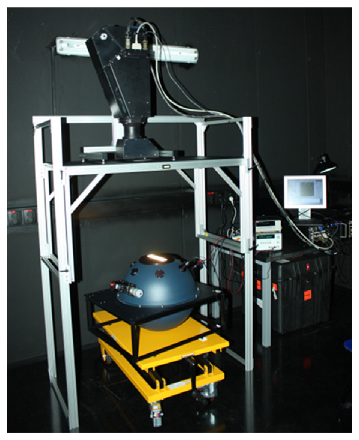
4.2.1. Radiometric Corrections

All hyperspectral sensors are under the ITRES maintenance programme and are regularly serviced and calibrated. Radiometric and spectral calibrations are performed every year by the sensor producer. Radiometric calibration parameters are determined for each pixel of the sensor matrix in a laboratory (Figure 4). The basic radiometric correction procedure for CASI and SASI data consists of subtracting dark current and converting raw values in digital numbers scanned by the sensor into physically defined radiance units. Radiometric corrections are performed using the RadCorr 12.1.3.0 software [48]. The values of the final image data are given in radiometric units [μW·cm−2·sr−1·nm−1] multiplied by a scaling factor of 1000 to make better use of the unsigned integer range.
Additional corrections can be applied to CASI and SASI hyperspectral data during the radiometric corrections to compensate for various negative artefacts in the data. For CASI data, the accuracy of the applied spectral correction is checked during the radiometric correction using a spectral calibration file produced on the fly by a built-in calibration source. Each CASI flight line is accompanied by a spectral calibration file measured before image data acquisition. The scattered light correction is particularly important for CASI, as it removes light scattered in the optical sensor system and is performed on individual rows using defined detector columns that do not receive the image signal. Frameshift smear correction addresses the added signal during data readout in the CCD detector. Second-order light correction adjusts the effect of the diffraction grating on the broad spectral range of the CASI sensor, which causes artificial amplification of the signal at specific wavelengths. This effect is corrected using a model based on laboratory experiments with the given sensor. Finally, residual correction, which uses homogenised uniformity data measured at the beginning and end of each flight line, can address random effects that influence individual pixels that cannot be removed during standard processing, such as dust particles on the detector.
For SASI data, additional spectral verification and corrections are based on atmospheric features. Correction of bad pixels is particularly important for SASI and TASI, which are equipped with mercury cadmium telluride detectors. This correction involves detecting and replacing the values of defective pixels with the interpolated values from the surrounding area in spatial or spectral dimensions. The total number of bad pixels is less than 1% of the total array for both sensors. The CASI sensor with the CCD detector has remained free from defective pixels, with only a few instances of bad pixels occurring since 2022 (less than 0.05%).

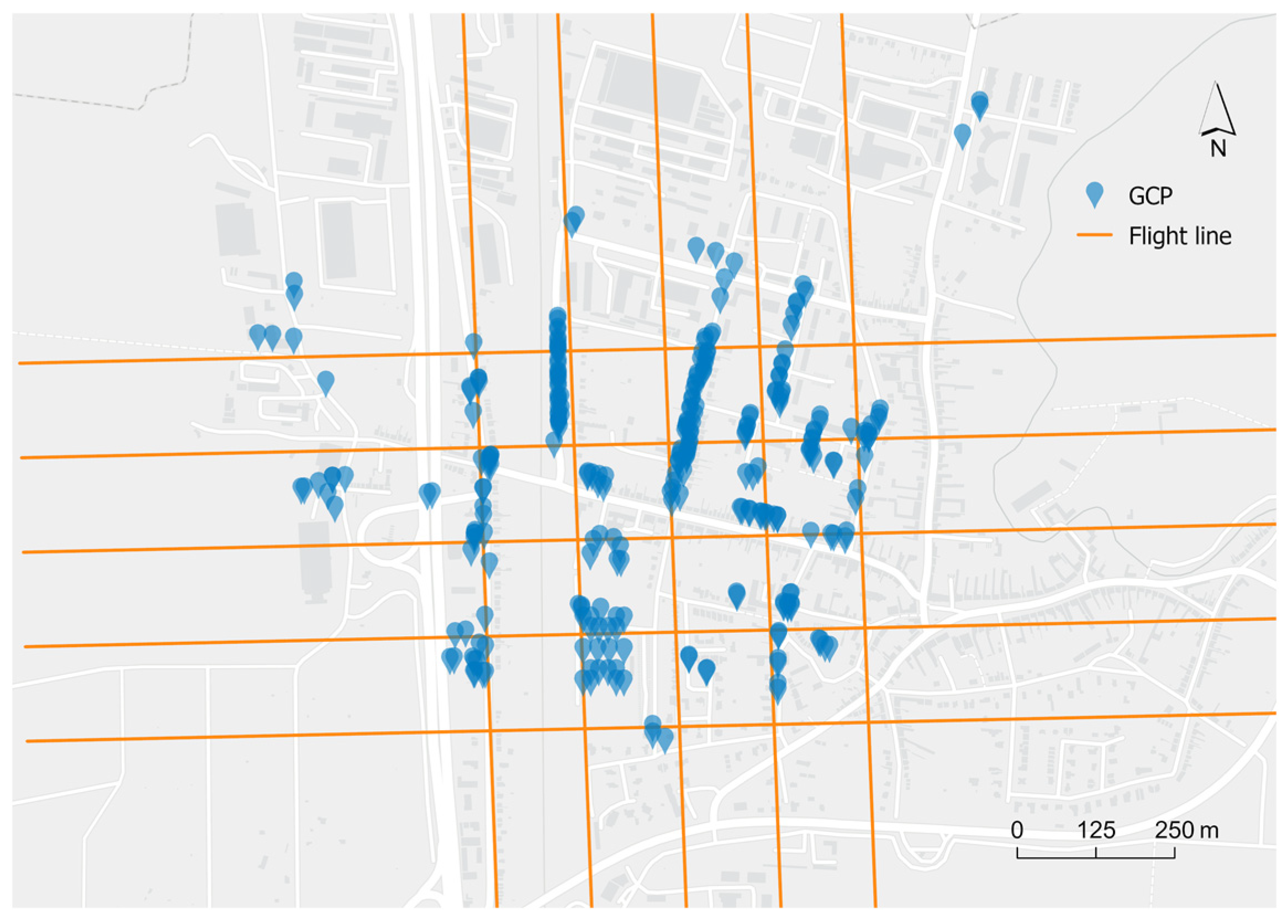
4.2.2. Georeferencing

Georeferencing, which includes geometric correction and orthorectification, is performed in a single step through parametric geocoding using auxiliary data logged by the POS AV 410 GNSS/IMU unit and a digital terrain model in the GeoCor 5.10.17.1 software [48]. The standard approach involves using a digital terrain model. For campaigns that target forest ecosystems, a digital surface model derived from the laser point cloud data is used to improve georeferencing accuracy. For the resampling of data to the coordinate system (ETRS-89, UTM), the nearest neighbour method is used to prevent spatial interpolation resulting in unrealistic spectral signatures [49,50]. If a mosaic is created, the min. nadir method is typically used, placing a pixel closer to the nadir from two overlapping lines into the mosaic. This mosaicking method reliably eliminates marginal pixels that are more affected by the BRDF effect.

4.2.3. Fusion of CASI and SASI Data

To fully utilise the VNIR-SWIR range for some spectral analysis, it is advantageous to aggregate CASI and SASI data into a single hyperspectral data cube. Due to different spatial resolutions, slightly different viewing angles (sensor models), and potential inaccuracies in georeferencing between CASI and SASI, there are discontinuities in a spectral profile at the VNIR-SWIR boundary [51,52]. Spectral discontinuities mainly occur on highly heterogeneous surfaces, such as forests with changes between sunlit and shaded pixels and urban areas with many spectrally different surfaces. For these ecosystems, it is not possible to use a simple pixel aggregate method to merge CASI and SASI hyperspectral cubes, which, on the other hand, works well for spectrally homogeneous surfaces such as meadows and crop fields. Therefore, we developed our own CASI-SASI Fuse (CSF) method optimised for forest areas.
The CSF method compares the overlapping spectral regions of CASI and SASI data. Input data to CSF are georeferenced and radiometrically corrected CASI and SASI hyperspectral cubes. In the first step, CASI data are spectrally resampled to the SASI spectral resolution and positions of the central wavelength using a third-order Butterworth filter. In the second step, the CASI data are resampled to match the SASI spatial resolution using the pixel aggregate method with a kernel size of 2.5 × 2.5 original CASI pixels. Pixel aggregation is calculated for 64 virtual positions, as illustrated in Figure 5. The original SASI pixel radiance is compared with the 49 variants of the averaged CASI radiance at the wavelength of 1004 nm (Figure 6). The virtual position with an average CASI radiance value that best matches the SASI radiance at 1004 nm is selected as the final position. Once the final spatial position of the CASI pixels for aggregation is determined, the original spectral resolution of the CASI data is used to compute the average radiance values, allowing the spatially resampled CASI data to maintain their original spectral resolution.
The CSF method is currently not optimised for urban systems with many small and spectrally different surfaces. For urban studies, the CASI and SASI datasets are analysed separately.
Figure 5. Schematic representation of the CASI-SASI Fuse (CSF) method. Thick black lines represent SASI pixels, and thin black lines represent CASI pixels. The CSF method creates 49 virtual positions of aggregated CASI pixels in SASI spatial resolution within the blue rectangle (the red kernel moves within the blue rectangle in steps of 0.5 CASI pixels). The final kernel position for CASI resampling is the minimum difference between the average CASI and SASI radiance values at 1004 nm.
Remotesensing 15 03130 g005
Figure 6. Example of the spectral radiance profile of a CASI-SASI fused pixel (red line) over a forested area. The black lines show a radiance variation of nine CASI pixels within one SASI pixel that would be used for a simple spatial pixel aggregation.
Remotesensing 15 03130 g006

4.2.4. Atmospheric Correction

Atmospheric corrections are based on a radiative transfer model that allows for the calculation of surface reflectance from at-sensor radiance without prior knowledge of surface reflectance properties. This calculation is divided into two parts: the estimation of atmospheric parameters and the calculation of surface reflectance. Key atmospheric parameters include the type and quantity of aerosols (aerosol optical thickness) and water vapour content, which significantly affect the passage of radiation through the atmosphere and can vary with time. These parameters can be measured using a sunphotometer during a ground support campaign or estimated directly from the image data.
Atmospheric corrections of CASI and SASI data are performed in the ATCOR-4 software package ver. 7.4.0 [47] using the MODTRAN4 radiative transfer model of the atmosphere [53,54]. Both path and adjacency radiances are corrected during the atmospheric corrections, and the resulting reflectance is calculated from the reflected radiance. The corrected data are expressed in reflectance values at the surface level (hemispherical-conical reflectance factor) multiplied by a constant of 100 to make better use of the unsigned integer range (a value of 1000 means a reflectance of 10%). An example of fully corrected CASI and CASI-SASI fused data is shown in Figure 7a,c.
Corrections for the BRDF effect caused by topography are necessary for data acquired over hilly terrain [47]. High-priority flight campaigns are usually accompanied by ground support measurements for verification/calibration purposes, including measurements of aerosol optical thickness, spectral measurements of ground reference targets, etc. [55]. Spectral reflectance field measurements could be used for vicarious calibration [56], which recalibrates the radiometric correction coefficients to the actual flight conditions, thus improving the atmospheric corrections performed within the ATCOR-4 software package.

4.3. TASI Data

4.3.1. Thermal Radiometric Corrections

The TASI sensor has a dual black body calibration system for onboard radiometric calibration. The first black body keeps an ambient temperature, while the second black body is heated to about 20 °C higher than the first black body. The onboard auxiliary radiometric calibration data are used for radiometric corrections performed in the RadCorr software [48]. There are two basic approaches to radiometric calibration. The first uses laboratory-determined calibration parameters when the onboard calibration data are obtained from a single black calibration body during the flight. The second approach, the dual black body method, uses calibration coefficients specific to each flight line using the data from two calibration black bodies scanned during the flight.
In most cases, the dual black body method is used. Data from the heated black body are also used for spectral verification or calibration of acquired TASI data. The accuracy of the spectral shift determined by the heated black body is significantly improved compared to the ambient black body data.
The values of the final image data are given in radiometric units [μW·cm−2·sr−1·nm−1] multiplied by a scaling factor of 1000 to make better use of the unsigned integer range.
In addition to the ITRES-recommended procedure to interpolate bad pixels in TASI, a two-step correction is applied to remove noise. In the first step, stripe noise is corrected in the spectral domain. In the second step, stochastic noise in the data is removed by spatial interpolation [57].

4.3.2. Thermal Atmospheric Corrections

The removal of atmospheric effects from the thermal hyperspectral data is essential for the correct retrieval of surface temperature and spectral emissivity. Radiometric calibrations deliver image data containing radiation from the surface attenuated by the atmosphere plus radiation from the atmosphere along the line of sight. Thus, the measured radiance at the sensor level (L) is expressed by the following radiative transfer equation:
L = τ ε   B ( T ) + τ ( 1 ε )   L atm + L atm
where τ is the atmospheric transmittance, ε is the surface’s emissivity, B(T) is the radiance of the surface at temperature T according to Planck’s law, L↓atm is the down-welling atmospheric radiance reflected by the surface (1 − ε), and L↑atm is the atmospheric up-welling radiance. All elements in the equation are wavelength dependent.
In our pre-processing chain, the quantities L↓atm, L↑atm and τ are modelled using the MODTRAN 5.3 radiative transfer model, which is parameterised using data from the ERA5 atmospheric near-real-time reanalysis provided by ECMWF [58]. ERA5 provides hourly estimates of a large number of atmospheric, land and oceanic climate variables on a 0.25° grid [59]. ERA5 data are spatially and temporally interpolated for each TASI flight line. Compensating for atmospheric transmittance and up-welling atmospheric radiance leads to land-leaving radiance:
LLL = ε B(T) + (1 − ε) L↓atm
LLL is the sum of the radiance emitted by the surface and the reflected radiance. Taking into account the down-welling atmospheric radiation L↓atm is not possible without knowing the surface’s emissivity. Eliminating the influence of down-welling atmospheric radiance is part of the calculation of temperature T (kinetic) and emissivity ε of the surface, which is performed by the Temperature and Emissivity Separation algorithm (TES).
TES was developed by Gillespie et al. (1998) [60] and evaluated in several studies [61,62,63,64], and it is used to resolve the indeterminacy of surface temperature and emissivity [65]. It relies on the assumption that any natural surface emissivity spectrum includes a value close to unity within the LWIR spectral range [66]. TES consists of three modules: the Normalization Emissivity Module [60], the Ratio Component and the Maximum-Minimum Difference Module [67]. In our TASI pre-processing chain, the Normalization Emissivity Module has been improved by smoothing spectral radiance signatures [68]. The Maximum-Minimum Difference module estimates real emissivity and temperature based on a semi-empirical relationship between emissivity contrast and minimum spectral emissivity for common materials [69]. It is meaningful to set its parameters according to the target area [70], so it can be tuned for agriculture, urban or forest areas of interest. To improve the TES’s accuracy, the noisiest bands can be excluded so that the final product has 22 bands. Typically, spectral bands 1–5 are removed due to noise induced by water vapour and bands 28–32 due to lower radiometric sensitivity.
The resulting images after the TASI atmospheric corrections are as follows:
  • Land surface temperature (kinetic temperature) [K] (Figure 7b);
  • Land surface emissivity [-];
  • Land leaving radiance [W m−2 sr−1 m−1];
  • Broadband brightness temperature for emissivity = 1 [K].

4.4. Laser Scanning Data

The pre-processing of the laser scanning data consists of several steps, which are executed using software tools provided by the laser scanner manufacturer, RIEGL Laser Measurement System GmbH. In the first step, the flight trajectory recorded by AP60 IMU/GNSS unit at a frequency of 200 Hz is calculated. Up until the 2020 flight season (included), data from the POS AV 410 INU/GNSS unit were used. This step is executed in the POSPac MMS 8.7 software. In the second step, points are extracted from the acquired full waveform data using RiUNITE 1.0.3. software. RiUNITE also combines data acquired by the scanner and IMU/GNSS unit. The final point cloud is exported into LAZ 1.4 format using the RiPROCESS 1.9.2 software. Data are exported in the ETRS-89 (UTM) coordinate system. The point cloud also includes Riegl extra bytes, which provide important information from full waveform analysis, such as amplitude and pulse width for each point. The final products derived from the point cloud data are the digital terrain model, digital surface model and normalised digital surface model (Figure 7d), which are calculated using the LasTools 20221102 software package.

5. Conclusions

We have established a fully operational airborne research infrastructure for multi-sensor observations to support complex ecological research. Our Flying Laboratory of Imaging Systems (FLIS) allows the simultaneous acquisition of VNIR-SWIR hyperspectral (CASI-1500 and SASI-600), LWIR thermal (TASI-600) and laser scanning (Riegl LMS Q780) data. The aircraft is also certified for HyPlant—the airborne demonstrator of the future FLEX satellite—and PTR-TOF 6000 for volatile organic compound measurements. FLIS data pre-processing is largely based on software tools provided by sensor manufacturers. Improvements and developments have been made in the pre-processing of TASI hyperspectral data and the fusion of CASI and SASI hyperspectral data cubes, mainly over heterogeneous forested areas. The pre-processing chain is currently well established, and further improvements will focus mainly on the better geometric fusion of sensor data and the timely delivery of final products to users.
FLIS operates in the European research space and is part of the EUFAR (European Facility for Airborne Research) association. Currently, the FLIS data are not openly distributed, but most of the acquisitions in the Czech Republic can be viewed at [71] and can be shared upon request for research purposes. The FLIS research infrastructure can be accessed either via EUFAR [72] or via open access to CzechGlobe’s research facilities [73].
The niche for aircraft-based remote sensing is getting narrower due to the recent expansion of unmanned aerial systems and the increasing availability of various satellite data. However, high-fidelity multi-sensor data from airborne platforms are still valuable. Airborne research platforms such as FLIS help to explore data synergies, develop new methods for ecosystem research, provide an intermediate link in an up-scaling scheme between field and satellite data and, finally, support calibration/validation activities of satellite missions. Airborne platforms are still the only platforms that simultaneously operate optical, thermal, radar, laser and other sensors under the same illumination conditions and provide data at a very high spatial resolution, which will not be achieved from space in the near future.

Author Contributions

Conceptualization, J.H., L.H. and L.S.; modelling, R.J. and D.K.; data visualisation, L.S., R.J. and J.H.; data curation, D.K., J.N., T.F., L.F., T.H., M.P., F.Z., K.P. and J.H.; writing—original draft preparation, J.H. and L.S. All authors made significant contributions to the review and editing of the draft. All authors have read and agreed to the published version of the manuscript.

Funding

This work was supported by the Ministry of Education, Youth and Sports of CR within the CzeCOS program, grant number LM2023048, Grant Agency of the Masaryk University (grant number MUNI/A/1323/2022) and by the internal grant CTU SGS23/052/OHK1/1T/11.

Data Availability Statement

Data are available upon request.

Conflicts of Interest

The authors declare no conflict of interest. The funders had no role in the development of the manuscript.

Appendix A

The anisotropic reflectance behaviour of vegetation was simulated for a virtual 3D spruce forest stand using the Discreet Anisotropic Radiative Transfer (DART) model version v1096 [74,75]. These simulations support and demonstrate how to minimise the BRDF effect when the flight plan is implemented in the actual solar principal plane. The virtual forest scene consists of 25 trees, each 15 m tall (Figure A1), with a tree LAI of 12 m2·m−2, reconstructed from terrestrial laser scanning data as described by Janoutová et al. (2021) [76]. The optical properties of the individual objects in the scene were set according to the field measurements described in Homolová et al. (2017) [77]. The size of the simulated scene was 10 × 10 m with a spatial resolution of 0.5 m; the sun’s zenith angle was 45° and the sun’s azimuth was 150°. Figure A2 shows the anisotropic behaviour of forest reflectance as a function of viewing geometry. Significant differences in reflectance as the viewing geometry changes can be seen in the solar principal plane. In contrast, minimal changes in reflectance occur in the direction perpendicular to the solar principal plane. The above-mentioned results can be advantageously applied to hyperspectral push-broom scanners that scan data in single lines. The only significant change in view angle is in the direction of the across-track. The most balanced reflectance values are therefore obtained when the flight plan is adjusted to the current position of the sun and the azimuth of the flight lines is very close to the current sun azimuth (i.e., the scan lines are perpendicular to the solar principal plane). Figure A3 shows how much a flight plan direction can deviate from the actual solar principal plane (sun azimuth). The lower graphs in Figure A3 show the minimal change in reflectance within the field of view of the FLIS hyperspectral sensors (from −20° to +20°) for planes oriented in a direction perpendicular to the solar principal plane or planes deviating up to 10°.
Figure A1. (a) 3D representation of the single spruce tree (side and nadir views); (b) schematic representation of the virtual forest scene used for radiative transfer simulations in the Discrete Anisotropic Radiative Transfer (DART) model.
Remotesensing 15 03130 g0a1
Figure A2. Simulation of the angular behaviour of the reflectance of a simulated Norway spruce forest at (a) 550 nm, (b) 665 nm, (c) 780 nm and (d) 1650 nm for the hemisphere. The white asterisk indicates the position of the sun at 45° zenith and 150° azimuth (0° zenith corresponds to the centre, 0° azimuth corresponds to the north). Simulations were performed using the Discrete Anisotropic Radiative Transfer (DART) model.
Remotesensing 15 03130 g0a2
Figure A3. Simulated spectral reflectance Bidirectional Reflectance Factor (BRF), as in Figure A2, but plotted for individual planes. The upper graphs show reflectance for the full range of viewing zenith angles across the hemisphere (from −90° to +90°). The lower graphs show reflectance within the field of view of the Flying Laboratory of Imaging Systems (FLIS) hyperspectral sensors (from −20° to +20°). The colours show the variation of the plane orientation relative to the sun azimuth angle in 5° steps (dark red—solar principal plane, dark green—plane perpendicular to solar principal plane).
Remotesensing 15 03130 g0a3

References

  1. Pettorelli, N.; Laurance, W.F.; O’Brien, T.G.; Wegmann, M.; Nagendra, H.; Turner, W. Satellite Remote Sensing for Applied Ecologists: Opportunities and Challenges. J. Appl. Ecol. 2014, 51, 839–848. [Google Scholar] [CrossRef]
  2. Ustin, S.L.; Middleton, E.M. Current and Near-Term Advances in Earth Observation for Ecological Applications. Ecol. Process. 2021, 10, 1. [Google Scholar] [CrossRef] [PubMed]
  3. Xiao, J.; Chevallier, F.; Gomez, C.; Guanter, L.; Hicke, J.A.; Huete, A.R.; Ichii, K.; Ni, W.; Pang, Y.; Rahman, A.F.; et al. Remote Sensing of the Terrestrial Carbon Cycle: A Review of Advances over 50 Years. Remote Sens. Environ. 2019, 233, 111383. [Google Scholar] [CrossRef]
  4. Farley, S.S.; Dawson, A.; Goring, S.J.; Williams, J.W. Situating Ecology as a Big-Data Science: Current Advances, Challenges, and Solutions. BioScience 2018, 68, 563–576. [Google Scholar] [CrossRef] [Green Version]
  5. Fisher, R.A.; Koven, C.D.; Anderegg, W.R.L.; Christoffersen, B.O.; Dietze, M.C.; Farrior, C.E.; Holm, J.A.; Hurtt, G.C.; Knox, R.G.; Lawrence, P.J.; et al. Vegetation Demographics in Earth System Models: A Review of Progress and Priorities. Glob. Chang. Biol. 2018, 24, 35–54. [Google Scholar] [CrossRef] [Green Version]
  6. Raffa, K.F.; Aukema, B.H.; Bentz, B.J.; Carroll, A.L.; Hicke, J.A.; Turner, M.G.; Romme, W.H. Cross-Scale Drivers of Natural Disturbances Prone to Anthropogenic Amplification: The Dynamics of Bark Beetle Eruptions. BioScience 2008, 58, 501–517. [Google Scholar] [CrossRef] [Green Version]
  7. Berger, K.; Machwitz, M.; Kycko, M.; Kefauver, S.C.; Van Wittenberghe, S.; Gerhards, M.; Verrelst, J.; Atzberger, C.; Van Der Tol, C.; Damm, A.; et al. Multi-Sensor Spectral Synergies for Crop Stress Detection and Monitoring in the Optical Domain: A Review. Remote Sens. Environ. 2022, 280, 113198. [Google Scholar] [CrossRef]
  8. Eitel, J.U.H.; Höfle, B.; Vierling, L.A.; Abellán, A.; Asner, G.P.; Deems, J.S.; Glennie, C.L.; Joerg, P.C.; LeWinter, A.L.; Magney, T.S.; et al. Beyond 3-D: The New Spectrum of Lidar Applications for Earth and Ecological Sciences. Remote Sens. Environ. 2016, 186, 372–392. [Google Scholar] [CrossRef] [Green Version]
  9. Kamoske, A.G.; Dahlin, K.M.; Read, Q.D.; Record, S.; Stark, S.C.; Serbin, S.P.; Zarnetske, P.L.; Dornelas, M. Towards Mapping Biodiversity from above: Can Fusing Lidar and Hyperspectral Remote Sensing Predict Taxonomic, Functional, and Phylogenetic Tree Diversity in Temperate Forests? Glob. Ecol. Biogeogr. 2022, 31, 1440–1460. [Google Scholar] [CrossRef]
  10. Lausch, A.; Borg, E.; Bumberger, J.; Dietrich, P.; Heurich, M.; Huth, A.; Jung, A.; Klenke, R.; Knapp, S.; Mollenhauer, H.; et al. Understanding Forest Health with Remote Sensing, Part III: Requirements for a Scalable Multi-Source Forest Health Monitoring Network Based on Data Science Approaches. Remote Sens. 2018, 10, 1120. [Google Scholar] [CrossRef] [Green Version]
  11. Senf, C. Seeing the System from Above: The Use and Potential of Remote Sensing for Studying Ecosystem Dynamics. Ecosystems 2022, 25, 1719–1737. [Google Scholar] [CrossRef]
  12. Hansen, M.C.; Potapov, P.V.; Moore, R.; Hancher, M.; Turubanova, S.A.; Tyukavina, A.; Thau, D.; Stehman, S.V.; Goetz, S.J.; Loveland, T.R.; et al. High-Resolution Global Maps of 21st-Century Forest Cover Change. Science 2013, 342, 850–853. [Google Scholar] [CrossRef] [PubMed] [Green Version]
  13. White, M.A.; de BEURS, K.M.; Didan, K.; Inouye, D.W.; Richardson, A.D.; Jensen, O.P.; O’Keefe, J.; Zhang, G.; Nemani, R.R.; van Leeuwen, W.J.D.; et al. Intercomparison, Interpretation, and Assessment of Spring Phenology in North America Estimated from Remote Sensing for 1982–2006. Glob. Chang. Biol. 2009, 15, 2335–2359. [Google Scholar] [CrossRef]
  14. Jung, M.; Reichstein, M.; Ciais, P.; Seneviratne, S.I.; Sheffield, J.; Goulden, M.L.; Bonan, G.; Cescatti, A.; Chen, J.; de Jeu, R.; et al. Recent Decline in the Global Land Evapotranspiration Trend Due to Limited Moisture Supply. Nature 2010, 467, 951–954. [Google Scholar] [CrossRef] [Green Version]
  15. Verrelst, J.; Rivera-Caicedo, J.P.; Reyes-Muñoz, P.; Morata, M.; Amin, E.; Tagliabue, G.; Panigada, C.; Hank, T.; Berger, K. Mapping Landscape Canopy Nitrogen Content from Space Using PRISMA Data. ISPRS J. Photogramm. Remote Sens. 2021, 178, 382–395. [Google Scholar] [CrossRef]
  16. Bachmann, M.; Alonso, K.; Carmona, E.; Gerasch, B.; Habermeyer, M.; Holzwarth, S.; Krawczyk, H.; Langheinrich, M.; Marshall, D.; Pato, M.; et al. Analysis-Ready Data from Hyperspectral Sensors—The Design of the EnMAP CARD4L-SR Data Product. Remote Sens. 2021, 13, 4536. [Google Scholar] [CrossRef]
  17. Curnick, D.J.; Davies, A.J.; Duncan, C.; Freeman, R.; Jacoby, D.M.P.; Shelley, H.T.E.; Rossi, C.; Wearn, O.R.; Williamson, M.J.; Pettorelli, N. SmallSats: A New Technological Frontier in Ecology and Conservation? Remote Sens. Ecol. Conserv. 2022, 8, 139–150. [Google Scholar] [CrossRef]
  18. Colomina, I.; Molina, P. Unmanned Aerial Systems for Photogrammetry and Remote Sensing: A Review. ISPRS J. Photogramm. Remote Sens. 2014, 92, 79–97. [Google Scholar] [CrossRef] [Green Version]
  19. Dainelli, R.; Toscano, P.; Di Gennaro, S.F.; Matese, A. Recent Advances in Unmanned Aerial Vehicle Forest Remote Sensing—A Systematic Review. Part I: A General Framework. Forests 2021, 12, 327. [Google Scholar] [CrossRef]
  20. Dainelli, R.; Toscano, P.; Di Gennaro, S.F.; Matese, A. Recent Advances in Unmanned Aerial Vehicles Forest Remote Sensing—A Systematic Review. Part II: Research Applications. Forests 2021, 12, 397. [Google Scholar] [CrossRef]
  21. Pavelka, K.; Raeva, P.; Pavelka, K. Evaluating the Performance of Airborne and Ground Sensors for Applications in Precision Agriculture: Enhancing the Postprocessing State-of-the-Art Algorithm. Sensors 2022, 22, 7693. [Google Scholar] [CrossRef] [PubMed]
  22. Pavelka, K.; Šedina, J.; Pavelka, K. Knud Rasmussen Glacier Status Analysis Based on Historical Data and Moving Detection Using RPAS. Appl. Sci. 2021, 11, 754. [Google Scholar] [CrossRef]
  23. Torresan, C.; Berton, A.; Carotenuto, F.; Di Gennaro, S.F.; Gioli, B.; Matese, A.; Miglietta, F.; Vagnoli, C.; Zaldei, A.; Wallace, L. Forestry Applications of UAVs in Europe: A Review. Int. J. Remote Sens. 2017, 38, 2427–2447. [Google Scholar] [CrossRef]
  24. Chadwick, K.; Asner, G. Organismic-Scale Remote Sensing of Canopy Foliar Traits in Lowland Tropical Forests. Remote Sens. 2016, 8, 87. [Google Scholar] [CrossRef] [Green Version]
  25. Cogliati, S.; Sarti, F.; Chiarantini, L.; Cosi, M.; Lorusso, R.; Lopinto, E.; Miglietta, F.; Genesio, L.; Guanter, L.; Damm, A.; et al. The PRISMA Imaging Spectroscopy Mission: Overview and First Performance Analysis. Remote Sens. Environ. 2021, 262, 112499. [Google Scholar] [CrossRef]
  26. Cooper, S.; Okujeni, A.; Pflugmacher, D.; Van Der Linden, S.; Hostert, P. Combining Simulated Hyperspectral EnMAP and Landsat Time Series for Forest Aboveground Biomass Mapping. Int. J. Appl. Earth Obs. Geoinf. 2021, 98, 102307. [Google Scholar] [CrossRef]
  27. Chlus, A.; Townsend, P.A. Characterizing Seasonal Variation in Foliar Biochemistry with Airborne Imaging Spectroscopy. Remote Sens. Environ. 2022, 275, 113023. [Google Scholar] [CrossRef]
  28. Novotný, J.; Navrátilová, B.; Janoutová, R.; Oulehle, F.; Homolová, L. Influence of Site-Specific Conditions on Estimation of Forest above Ground Biomass from Airborne Laser Scanning. Forests 2020, 11, 268. [Google Scholar] [CrossRef] [Green Version]
  29. Chadwick, K.D.; Brodrick, P.G.; Grant, K.; Goulden, T.; Henderson, A.; Falco, N.; Wainwright, H.; Williams, K.H.; Bill, M.; Breckheimer, I.; et al. Integrating Airborne Remote Sensing and Field Campaigns for Ecology and Earth System Science. Methods Ecol. Evol. 2020, 11, 1492–1508. [Google Scholar] [CrossRef]
  30. Forzieri, G.; Tanteri, L.; Moser, G.; Catani, F. Mapping Natural and Urban Environments Using Airborne Multi-Sensor ADS40–MIVIS–LiDAR Synergies. Int. J. Appl. Earth Obs. Geoinf. 2013, 23, 313–323. [Google Scholar] [CrossRef]
  31. Urban, J.; Pikl, M.; Zemek, F.; Novotný, J. Using Google Street View Photographs to Assess Long-Term Outdoor Thermal Perception and Thermal Comfort in the Urban Environment during Heatwaves. Front. Environ. Sci. 2022, 10, 878341. [Google Scholar] [CrossRef]
  32. Asner, G.P. Carnegie Airborne Observatory: In-Flight Fusion of Hyperspectral Imaging and Waveform Light Detection and Ranging for Three-Dimensional Studies of Ecosystems. J. Appl. Remote Sens. 2007, 1, 013536. [Google Scholar] [CrossRef]
  33. Asner, G.P.; Knapp, D.E.; Boardman, J.; Green, R.O.; Kennedy-Bowdoin, T.; Eastwood, M.; Martin, R.E.; Anderson, C.; Field, C.B. Carnegie Airborne Observatory-2: Increasing Science Data Dimensionality via High-Fidelity Multi-Sensor Fusion. Remote Sens. Environ. 2012, 124, 454–465. [Google Scholar] [CrossRef]
  34. Kampe, T.U. NEON: The First Continental-Scale Ecological Observatory with Airborne Remote Sensing of Vegetation Canopy Biochemistry and Structure. J. Appl. Remote Sens. 2010, 4, 043510. [Google Scholar] [CrossRef] [Green Version]
  35. Cook, B.; Corp, L.; Nelson, R.; Middleton, E.; Morton, D.; McCorkel, J.; Masek, J.; Ranson, K.; Ly, V.; Montesano, P. NASA Goddard’s LiDAR, Hyperspectral and Thermal (G-LiHT) Airborne Imager. Remote Sens. 2013, 5, 4045–4066. [Google Scholar] [CrossRef] [Green Version]
  36. ARES|Airborne Research of the Earth System. Available online: https://ares-observatory.ch/ (accessed on 7 June 2023).
  37. NEODAAS-Airborne. Available online: https://nerc-arf-dan.pml.ac.uk/ (accessed on 7 June 2023).
  38. FLIS—Department of Airborne Activities. Available online: https://olc.czechglobe.cz/en/flis-2/ (accessed on 8 June 2023).
  39. Hanuš, J.; Fabiánek, T.; Fajmon, L. Potential of Airborne Imaging Spectroscopy at CzechGlobe. ISPRS Int. Arch. Photogramm. Remote Sens. Spat. Inf. Sci. 2016, XLI-B1, 15–17. [Google Scholar] [CrossRef]
  40. Riegl. Airborne Laser Scanner LMS-Q780 General Description and Data Interface (Manual); Riegl: Horn, Austria, 2014. [Google Scholar]
  41. CzechGlobe|Virtual Tour. Available online: http://czechglobe.pano3d.eu (accessed on 8 June 2023).
  42. Rascher, U.; Alonso, L.; Burkart, A.; Cilia, C.; Cogliati, S.; Colombo, R.; Damm, A.; Drusch, M.; Guanter, L.; Hanus, J.; et al. Sun-Induced Fluorescence—A New Probe of Photosynthesis: First Maps from the Imaging Spectrometer HyPlant. Glob. Chang. Biol. 2015, 21, 4673–4684. [Google Scholar] [CrossRef] [Green Version]
  43. Siegmann, B.; Alonso, L.; Celesti, M.; Cogliati, S.; Colombo, R.; Damm, A.; Douglas, S.; Guanter, L.; Hanuš, J.; Kataja, K.; et al. The High-Performance Airborne Imaging Spectrometer HyPlant—From Raw Images to Top-of-Canopy Reflectance and Fluorescence Products: Introduction of an Automatized Processing Chain. Remote Sens. 2019, 11, 2760. [Google Scholar] [CrossRef] [Green Version]
  44. FLEX—Earth Online. Available online: https://earth.esa.int/eogateway/missions/flex (accessed on 23 March 2023).
  45. Launching the Revolutionary PTR-TOF 6000 X2 Trace VOC Analyzer|IONICON. Available online: https://www.ionicon.com/blog/2017/launching-the-revolutionary-ptr-tof-6000-x2-trace-voc-analyzer (accessed on 17 May 2023).
  46. Dashora, A.; Lohani, B.; Deb, K. Two-Step Procedure of Optimisation for Flight Planning Problem for Airborne LiDAR Data Acquisition. Int. J. Math. Model. Numer. Optim. 2013, 4, 323. [Google Scholar] [CrossRef]
  47. Richter, R.; Schläpfer, D. Atmospheric/Topographic Correction for Airborne Imagery (ATCOR-4 User Guide) 2021; ReSe Applications LLC: Langeggweg, Switzerland, 2021. [Google Scholar]
  48. Itres. Standard Processing and Data QA Manual; Itres: Calgary, AB, Canada, 2013. [Google Scholar]
  49. Richter, R.; Schläpfer, D. Geo-Atmospheric Processing of Airborne Imaging Spectrometry Data. Part 2: Atmospheric/Topographic Correction. Int. J. Remote Sens. 2002, 23, 2631–2649. [Google Scholar] [CrossRef]
  50. Schläpfer, D.; Richter, R. Geo-Atmospheric Processing of Airborne Imaging Spectrometry Data. Part 1: Parametric Orthorectification. Int. J. Remote Sens. 2002, 23, 2609–2630. [Google Scholar] [CrossRef]
  51. Inamdar, D.; Kalacska, M.; Darko, P.O.; Arroyo-Mora, J.P.; Leblanc, G. Spatial Response Resampling (SR2): Accounting for the Spatial Point Spread Function in Hyperspectral Image Resampling. MethodsX 2023, 10, 101998. [Google Scholar] [CrossRef] [PubMed]
  52. Yang, H.; Zhang, L.; Ong, C.; Rodger, A.; Liu, J.; Sun, X.; Zhang, H.; Jian, X.; Tong, Q. Improved Aerosol Optical Thickness, Columnar Water Vapor, and Surface Reflectance Retrieval from Combined CASI and SASI Airborne Hyperspectral Sensors. Remote Sens. 2017, 9, 217. [Google Scholar] [CrossRef] [Green Version]
  53. Berk, A.; Anderson, G.P.; Bernstein, L.S.; Acharya, P.K.; Dothe, H.; Matthew, M.W.; Adler-Golden, S.M.; Chetwynd, J.H., Jr.; Richtsmeier, S.C.; Pukall, B.; et al. MODTRAN4 radiative transfer modeling for atmospheric correction. In Proceedings of the 1999 SPIE’s International Symposium on Optical Science Engineering, and Instrumentation, Denver, CO, USA, 18–23 July 1999; p. 348. [Google Scholar] [CrossRef]
  54. Guanter, L.; Gómez-Chova, L.; Moreno, J. Coupled Retrieval of Aerosol Optical Thickness, Columnar Water Vapor and Surface Reflectance Maps from ENVISAT/MERIS Data over Land. Remote Sens. Environ. 2008, 112, 2898–2913. [Google Scholar] [CrossRef]
  55. Green, R.O.; Conel, J.E.; Margolis, J.; Chovit, C.; Faust, J. In-Flight Calibration and Validation of the Airborne Visible/Infrared Imaging Spectrometer (AVIRIS). 1996. Available online: https://hdl.handle.net/2014/25023 (accessed on 20 May 2023).
  56. Secker, J.; Staenz, K.; Gauthier, R.P.; Budkewitsch, P. Vicarious Calibration of Airborne Hyperspectral Sensors in Operational Environments. Remote Sens. Environ. 2001, 76, 81–92. [Google Scholar] [CrossRef]
  57. He, W.; Yao, Q.; Li, C.; Yokoya, N.; Zhao, Q. Non-Local Meets Global: An Integrated Paradigm for Hyperspectral Denoising. In Proceedings of the 2019 IEEE/CVF Conference on Computer Vision and Pattern Recognition (CVPR), Long Beach, CA, USA, 15–20 June 2019; pp. 6861–6870. [Google Scholar]
  58. Copernicus|Climate Data Store. Available online: https://cds.climate.copernicus.eu/#!/home (accessed on 8 June 2023).
  59. Guillory, A. ERA5. Available online: https://www.ecmwf.int/en/forecasts/datasets/reanalysis-datasets/era5 (accessed on 23 March 2023).
  60. Gillespie, A.; Rokugawa, S.; Matsunaga, T.; Cothern, J.S.; Hook, S.; Kahle, A.B. A Temperature and Emissivity Separation Algorithm for Advanced Spaceborne Thermal Emission and Reflection Radiometer (ASTER) Images. IEEE Trans. Geosci. Remote Sens. 1998, 36, 1113–1126. [Google Scholar] [CrossRef]
  61. Cheng, J.; Liang, S.; Wang, J.; Li, X. A Stepwise Refining Algorithm of Temperature and Emissivity Separation for Hyperspectral Thermal Infrared Data. IEEE Trans. Geosci. Remote Sens. 2010, 48, 1588–1597. [Google Scholar] [CrossRef]
  62. Kealy, P.S.; Hook, S.J. Separating Temperature and Emissivity in Thermal Infrared Multispectral Scanner Data: Implications for Recovering Land Surface Temperatures. IEEE Trans. Geosci. Remote Sens. 1993, 31, 1155–1164. [Google Scholar] [CrossRef]
  63. Sobrino, J.A.; Jimenez-Munoz, J.C.; Soria, G.; Romaguera, M.; Guanter, L.; Moreno, J.; Plaza, A.; Martinez, P. Land Surface Emissivity Retrieval From Different VNIR and TIR Sensors. IEEE Trans. Geosci. Remote Sens. 2008, 46, 316–327. [Google Scholar] [CrossRef]
  64. Vermote, E.F.; Tanre, D.; Deuze, J.L.; Herman, M.; Morcette, J.-J. Second Simulation of the Satellite Signal in the Solar Spectrum, 6S: An Overview. IEEE Trans. Geosci. Remote Sens. 1997, 35, 675–686. [Google Scholar] [CrossRef] [Green Version]
  65. Pérez-Planells, L.; Valor, E.; Coll, C.; Niclòs, R. Comparison and Evaluation of the TES and ANEM Algorithms for Land Surface Temperature and Emissivity Separation over the Area of Valencia, Spain. Remote Sens. 2017, 9, 1251. [Google Scholar] [CrossRef] [Green Version]
  66. Payan, V.; Royer, A. Analysis of Temperature Emissivity Separation (TES) Algorithm Applicability and Sensitivity. Int. J. Remote Sens. 2004, 25, 15–37. [Google Scholar] [CrossRef]
  67. Matsunaga, T. A Temperature-Emissivity Separation Method Using an Empirical Relationship between the Mean, the Maximum, and the Minimum of the Thermal Infrared Emissivity Spectrum. J. Remote Sens. Soc. Jpn. 1994, 14, 230–241. [Google Scholar]
  68. Pivovarnik, M. New Approaches in Airborne Thermal Image Processing for Landscape Assessment. Ph.D. Thesis, Brno University of Technology, Brno, Czech Republic, 2017. [Google Scholar]
  69. Sabol, D.E., Jr.; Gillespie, A.R.; Abbott, E.; Yamada, G. Field Validation of the ASTER Temperature–Emissivity Separation Algorithm. Remote Sens. Environ. 2009, 113, 2328–2344. [Google Scholar] [CrossRef]
  70. Michel, A.; Granero-Belinchon, C.; Cassante, C.; Boitard, P.; Briottet, X.; Adeline, K.R.M.; Poutier, L.; Sobrino, J.A. A New Material-Oriented TES for Land Surface Temperature and SUHI Retrieval in Urban Areas: Case Study over Madrid in the Framework of the Future TRISHNA Mission. Remote Sens. 2021, 13, 5139. [Google Scholar] [CrossRef]
  71. Mapserver CzechGlobe. Available online: https://mapserver.czechglobe.cz/en/map (accessed on 8 June 2023).
  72. EUFAR—The EUropean Facility for Airborne Research. Available online: http://eufar.net/ (accessed on 8 June 2023).
  73. Open Access to CzeCOS Research Infrastructure Hosted byGlobal Change Research Institute CAS. Available online: https://www.czechglobe.cz/en/open-access-en/czecos-en/ (accessed on 8 June 2023).
  74. Gastellu-Etchegorry, J.-P.; Lauret, N.; Yin, T.; Landier, L.; Kallel, A.; Malenovsky, Z.; Bitar, A.A.; Aval, J.; Benhmida, S.; Qi, J.; et al. DART: Recent Advances in Remote Sensing Data Modeling With Atmosphere, Polarization, and Chlorophyll Fluorescence. IEEE J. Sel. Top. Appl. Earth Obs. Remote Sens. 2017, 10, 2640–2649. [Google Scholar] [CrossRef]
  75. Malenovský, Z.; Regaieg, O.; Yin, T.; Lauret, N.; Guilleux, J.; Chavanon, E.; Duran, N.; Janoutová, R.; Delavois, A.; Meynier, J.; et al. Discrete Anisotropic Radiative Transfer Modelling of Solar-Induced Chlorophyll Fluorescence: Structural Impacts in Geometrically Explicit Vegetation Canopies. Remote Sens. Environ. 2021, 263, 112564. [Google Scholar] [CrossRef]
  76. Janoutová, R.; Homolová, L.; Novotný, J.; Navrátilová, B.; Pikl, M.; Malenovský, Z. Detailed Reconstruction of Trees from Terrestrial Laser Scans for Remote Sensing and Radiative Transfer Modelling Applications. Silico Plants 2021, 3, diab026. [Google Scholar] [CrossRef]
  77. Homolová, L.; Janoutová, R.; Lukeš, P.; Hanuš, J.; Novotný, J.; Brovkina, O.; Loayza Fernandez, R.R. In Situ Data Supporting Remote Sensing Estimation of Spruce Forest Parameters at the Ecosystem Station Bílý Kříž. Beskydy 2018, 10, 75–86. [Google Scholar] [CrossRef] [Green Version]
Figure 1. (a) Cessna 208 B Grand Caravan airborne carrier and (b) the instruments onboard (from right to left: LSM Q780 laser scanner, TASI-600, CASI-1500 and SASI-600 on a gyro-stabilised platform, a rack with acquisition computers).
Remotesensing 15 03130 g001
Figure 2. Flow chart of the Flying Laboratory of Imaging Systems (FLIS) data pre-processing chains for CASI, SASI, and TASI imaging spectroscopy data and for laser scanning (LiDAR) data. Abbreviations: GNSS—Global Navigation Satellite System; IMU—Inertial Measurement Unit; DTM—Digital Terrain Model; DSM—Digital Surface Model; nDSM—normalised DSM; Surf. refl.—Surface reflectance; ε—Emissivity; BBT—Broadband Brightness Temperature; LST—Land Surface Temperature.
Remotesensing 15 03130 g002
Figure 3. Overview of the boresight calibration site in Brno district Modřice (49.1289N, 16.6094E) with about 400 ground control points (GCP) and a calibration flight plan for hyperspectral sensors.
Remotesensing 15 03130 g003
Figure 4. Laboratory determination of radiometric calibration coefficients for the SASI-600 sensor using the LabSphere CSTM-LR-20-M-C integrating sphere at the CzechGlobe calibration premises.
Remotesensing 15 03130 g004
Figure 7. Example of the Flying Laboratory of Imaging Systems (FLIS) final products: (a) VNIR hyperspectral data obtained from CASI (displayed as the true-colour composite, pixel size of 0.5 m); (b) land surface temperature obtained from TASI (pixel size of 1.25 m); (c) VNIR-SWIR hyperspectral data obtained by the fusion of CASI and SASI data (displayed as the false-colour composite R—725 nm, G—652 nm, B—552 nm, pixel size of 1.25 m); and (d) normalised digital surface model obtained from the laser scanner (pixel size of 0.5 m).
Remotesensing 15 03130 g007
Table 1. Basic technical specifications of the FLIS hyperspectral instruments.
CASI-1500SASI-600TASI-600
Spectral domainVNIRSWIRLWIR
Spectral range [nm]380–1050950–24508000–11,500
Max. spectral resolution [nm]2.715110
Max. number of spectral bands28810032
Across-track spatial pixels1500600600
Field of view [°]404040
Instantaneous field of view [mrad]0.491.21.2
Typical spatial resolution 1 [m]0.5–2.01.25–5.01.25–5.0
1 The minimum spatial resolution corresponds to the flight altitude of about 1000 m above ground level (AGL), while the maximum corresponds to 4000 m AGL.
Table 2. Basic technical specifications of the FLIS airborne laser scanner LMS Q780.
LMS Q780
Laser pulse repetition rate [kHz]Up to 400
Maximum measuring range [m]Up to 5800 1
Wavelength [nm]1064
Laser beam divergence [mrad]≤0.25
Field of view [°]60
Typical point density [pts/m2]0.5–4 2
1 For targets with 60% reflectivity, for targets with 20% reflectivity the maximum range is 4100 m. The maximum range is also dependent on atmospheric conditions. 2 The minimum point density of 0.5 pts/m2 corresponds to the flight altitude of 4000 m AGL, and the maximum of 4 pts/m2 to 1000 AGL. Due to flight line overlap, point densities are usually between 1 and 8 pts/m2.
Disclaimer/Publisher’s Note: The statements, opinions and data contained in all publications are solely those of the individual author(s) and contributor(s) and not of MDPI and/or the editor(s). MDPI and/or the editor(s) disclaim responsibility for any injury to people or property resulting from any ideas, methods, instructions or products referred to in the content.

