
Analysis of Two Convective Storms Using Polarimetric X-Band Radar and Satellite Data


1
Institute of Atmospheric Physics of the Czech Academy of Sciences, Bocni II 1401, 141 00 Prague, Czech Republic
2
Faculty of Environmental Sciences, Czech University of Life Sciences, Kamýcká 1176, 165 00 Prague, Czech Republic
3
Faculty of Science, Charles University, Albertov 6, 128 00 Prague, Czech Republic
4
Faculty of Electrical Engineering and Informatics, University of Pardubice, Studentská 95, 532 10 Pardubice, Czech Republic
*
Author to whom correspondence should be addressed.
Remote Sens. 2022, 14(10), 2294; https://doi.org/10.3390/rs14102294
Submission received: 30 March 2022
/
Revised: 25 April 2022
/
Accepted: 6 May 2022
/
Published: 10 May 2022
(This article belongs to the Special Issue Radar Remote Sensing: Retrieval Algorithms and Applications for Characterizing Precipitation)
Abstract
:We analyzed two convective storms that passed over or near the Milešovka meteorological observatory. The observatory is located at the top of a hill and has been recently equipped with a Doppler polarimetric X-band radar FURUNO WR2120 for cloud investigations. Our analysis was based mainly on Doppler polarimetric radar data measured in vertical cross-sections (RHI-Range-Height Indicator). Radar data was also used for classifying hydrometeors by a newly developed XCLASS (X-band radar CLASSification) algorithm. We also used rapid scan data measured by the geostationary satellite Meteosat Second Generation to validate radar measurements at the upper parts of storms. Although an attenuation correction was applied to the reflectivity and differential reflectivity measurements, the attenuation typical of X-band radars was noticeable. It was mainly manifested in the differential reflectivity, co-polar correlation coefficient and specific differential phase. Nevertheless, radar measurements can be used to analyze the internal cloud structure of severe convective storms. The XCLASS classification was developed by major innovation of a previously published algorithm. The XCLASS algorithm identifies seven types of hydrometeors: light rain, rain, wet snow, dry snow, ice, graupel, and hail. It uses measured horizontal and vertical radar reflectivity, specific differential phase, co-polar correlation coefficient, and temperature, and applies fuzzy logic to determine the type of hydrometeor. The new algorithm practically eliminates unrealistic results around and below the melting layer provided by the original algorithm. It identifies wet snow in more cases, and areas with individual hydrometeors have more realistic shapes compared to the original algorithm. The XCLASS algorithm shows reasonable results for the classification of hydrometeors and can be used to study the structure of convective storms.
1. Introduction
Convective weather may cause severe meteorological phenomena that can endanger human lives and lead to significant economic damages yearly. Severe convective phenomena, which occur in Central Europe include, in particular, intense rainfall accompanied by flash floods, strong winds, extreme wind gusts, lightning, and, in exceptional cases, tornadoes also [1,2,3,4,5]. Therefore, considerable attention has been paid to the research of convection, where radar and satellite remote sensing devices play a crucial role due to the hard predictability of convective phenomena.
Radars and satellite measurements, including airborne radars, complement each other as they monitor storms from different directions. The mutual use of radar and satellite data in cloud and storm research can be found in numerous papers. Moreover, these data are also used in weather forecasting. Meteorological satellites and radars are suitable for monitoring the current state of the atmosphere, for remote exploration of clouds and cloud-related phenomena, such as storm structures, and for investigating the relationships between clouds and lightning in the atmosphere. The joint use of radar and satellite measurements began in the 1970s and 1980s, e.g., [6], and has further continued with technological progress in the measuring instruments.
Studies [7,8,9,10,11,12,13,14,15,16,17,18,19] provide examples of the use of both radar and satellite measurements for remote atmospheric research from recent times. These studies are focused on analysis of single events or try to find the general characteristics of studied events. Putsay et al. [7] studied a mesoscale convective system crossing Hungary and causing severe weather, including hail, using satellites, radars and a lightning detection system. They showed that composites of these data helped to assess the relative locations of the main up- and downdrafts and other important features of the severe storm. Mathee et al. [8] performed analyses of Meteosat Second Generation geostationary satellite data and S-band NASA Polarimetric Doppler Weather Radar data with the aim of increas understanding of the relationships between lightning and non-lightning convective storms. Hu et al. [9] dealt with analysis of the microphysics and precipitation patterns of two hurricanes (Harvey 2017 and Florence 2018) using satellite and radar data.
Mulholland et al. [10] made use of satellite observations and C-band dual-polarization Doppler weather radar data from two years of spring and summer seasons to document the convective life cycle and estimate the storm environment in the region Sierras de Córdoba, Argentina, South America, and Murrilo and Homeyer [11] analyzed more than 10,000 storms using NEXRAD radar dual-polarization and geostationary satellites, with spatiotemporal resolution comparable to that of NEXRAD data, to improve discrimination between severe and non-severe hailstorms and identification of individual hail occurrence. Sandmael et al. [12] used three large-area datasets, which included a geostationary satellite, ground-based radar, and ground-based lightning detection data, to attempt to objectively discriminate between severe and non-severe storms for the US territory.
Radar and satellite data are used in conjunction with high-resolution numerical models either to prepare boundary conditions or to validate model outputs and study cloud microphysics. As an example, Jones et al. [13] used combination of high-resolution radar reflectivity and radial velocity together with a Geostationary Operational Environmental Satellite cloud water path as assimilated data into a convection-permitting numerical weather prediction model and proved that these data improved the skill of convection forecasting. Khan et al. [14] applied Doppler weather radar and Indian National Satellite 3D Repeat (INSAT 3DR) satellite observations to study cloud characteristics and the results compared with the simulations of the Weather Research and Forecasting model. Manzato et al. [15] used various observations, including Doppler radar, extra-soundings, sodar, surface stations, 2.5-min rapid scan with the Meteosat Second Generation 3 satellite, and simulations by numerical weather prediction models, to identify factors responsible for the initiation of severe convection that occurred in the north-eastern part of Italy.
In this article, we analyze two convective storms which passed near or over the Milešovka meteorological observatory, situated in Central Europe, in 2021, and were associated with significant lightning activity in the vicinity of the observatory. We study these events using the FURUNO X-band weather radar installed at the Milešovka meteorological observatory as a primary source of data. Data measured by the geostationary satellite Meteosat Second Generation (MSG) and standard meteorological observations are complementary data in this study. The FURUNO X-band weather radar is a research radar aimed at research on clouds and especially exploration of convective storms accompanied by lightning. Cloud electrification and lightning generation is our long-term research focus [16,17].
Our study has two main objectives. The first objective is to analyse severe convective storms using the X-band radar and to test the capabilities and limitations of these measurements. In doing so, we focus primarily on vertical scanning of storms and the corresponding cloud structures. The second objective is the development and validation of the XCLASS algorithm designed for hydrometeor classification.
This paper is organized as follows. After this introductory section, Section 2 shows the location and equipment of the Milešovka meteorological observatory and presents the data processing including the newly developed X-band radar CLASSification algorithm (XCLASS), which we use to classify hydrometeors in convective clouds. Section 3 provides description and analysis of the two studied convective events using XCLASS, standard meteorological data, and satellite data. Section 4 discusses the obtained results, while Section 5 contains the main conclusions of our study.
2. Data
2.1. Milešovka Meteorological Observatory
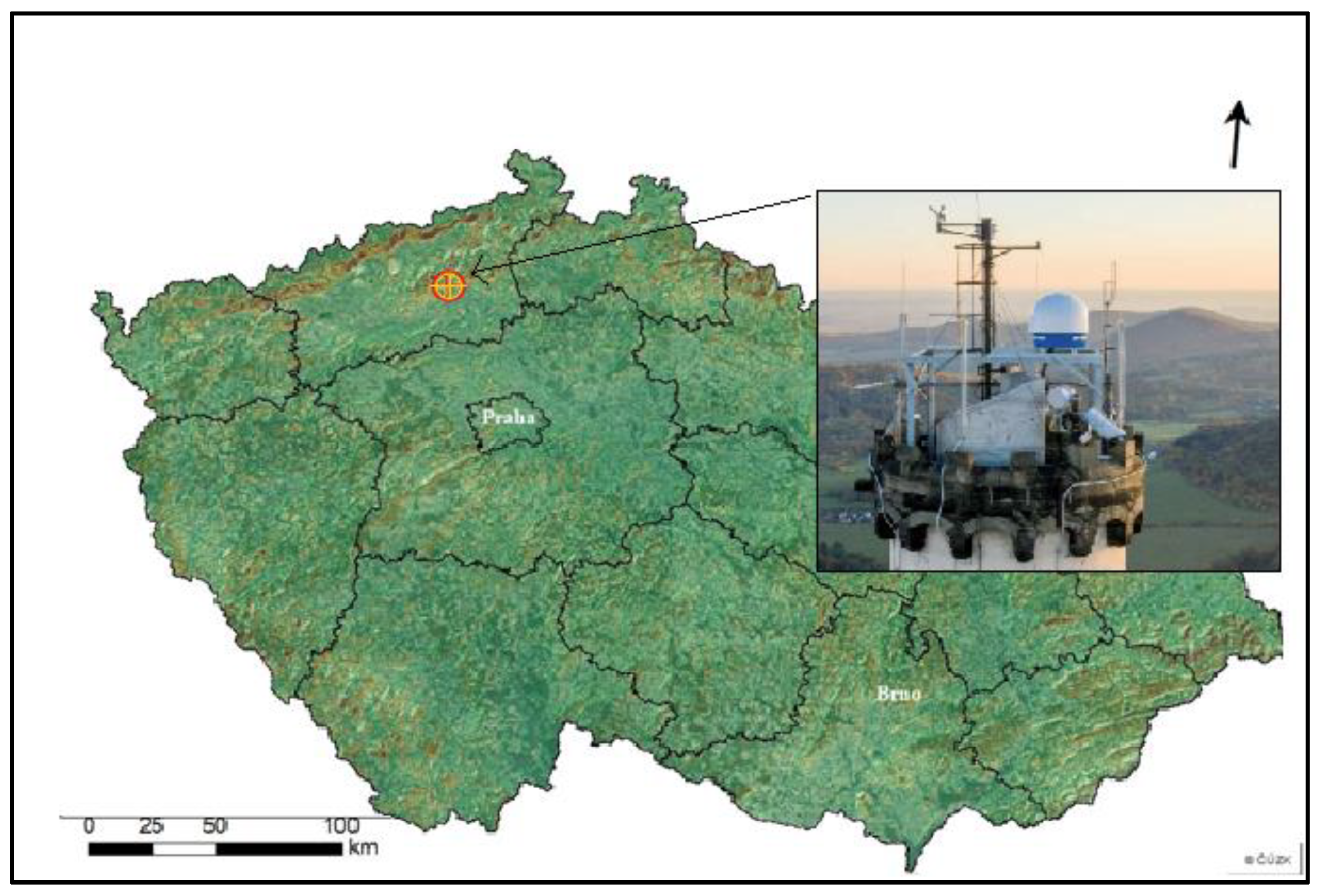
The Milešovka meteorological observatory (50°33′17″ N, 13°55′57″ E, 837 m a.s.l.), which is operated by the Institute of Atmospheric Physics of the Czech Academy of Sciences, is located in the northern part of the Czech Republic (Central Europe) at the top of the Milešovka mountain, the landmark of the Bohemian Central Highlands (Figure 1).
The observatory provides routine and specific meteorological and climatological measurements with a 24/7 service and its location is suitable for atmospheric research due to a large 360° view and an absence of tall obstacles in the surroundings. This feature, as well as a long-term series of measurements (since 1905), make the observatory unique in the European context.
The equipment of the Milešovka observatory comprises instruments of a standard meteorological and climatological observatory providing, e.g., measurements of pressure, temperature (including underground temperatures), humidity, wind direction and speed, precipitation, and cloud characteristics. Among others, it also includes two sonic anemometers, Vaisala ceilometer CL51 and Thies Laser Precipitation Monitor. Besides various meteorological instruments, the Milešovka observatory has been equipped with instruments measuring the atmospheric electric field (Boltek Electric Field Monitor EFM-100), the magnetic field (SLAVIA sensors, Shielded Loop Antenna with a Versatile Integrated Amplifier), and charged and neutral components of secondary cosmic rays (SEVAN) in order to investigate lightning in thunderstorms. In late 2020, a FURUNO X-band weather radar was placed on the observatory tower (Figure 1), providing operational measurements since 2021.
2.2. FURUNO X-Band Weather Radar and Its Data
The FURUNO weather radar installed at the Milešovka observatory (FURUNO WR2120) in late 2020 is a Doppler polarimetric X-band radar. Its basic parameters are given in Table 1. The radar is located at the top of the observatory tower (Figure 1), which provides an unobstructed view of the surroundings with the exception of the few metal rods needed for other measuring devices placed on the tower that cannot be removed due to the need for maintaining measuring continuity. Our experience regarding the operation of the radar since 2021 has shown that these metal rods probably cause, under certain conditions, artefacts in the radar measurements, which are manifested at higher elevations and in the vicinity of the radar, and are currently being solved in cooperation with the radar manufacturer. The artefacts are not standard errors in radar measurements, which are known, thus standard automatic corrections, e.g., [18], cannot be applied. As we are interested in the microphysical processes of convective clouds and their relation to cloud electrification, we focus on the data from the mid and upper troposphere, so the described artefacts are not crucial for us.
The radar scanning strategy consists of two steps: (i) the radar performs 7 horizontal ppi (plan position indicator) clockwise scans for elevations of 1.1°, 1.7°, 2.5°, 4°, 6°, 10° and 25°; (ii) the radar makes 6 RHI (range height indicator) scans, i.e., 6 vertical cross section scans, for elevation angles from 3° to 90°. The difference between adjacent elevation angles is non-equidistant but not larger than 0.5°. The azimuths of the scans are set in a way that they can be folded into three cross sections, the first of which is oriented from south to north, the second rotated 60° clockwise to the first, and the third rotated 120° to the first.
We set the radar scanning strategy to correspond to our research of summer convective clouds which occur near and above the Milešovka meteorological observatory. Specifically, we combine PPI and RHI scans and use the final scan parameters resulting from a trade-off between two following contradictory requirements: (i) to perform as many spatial measurements as possible, which is important due to the local character of convective phenomena; and (ii) to obtain the highest possible time resolution, which is important due to the rapid development of the convective phenomena.
The lowest PPI scan is set relatively high intentionally since our primary target is not precipitation estimatation in the radar domain but investigation of cloud structure. In addition, the mountain ridge, with heights of about 1000 m at a distance of about 10 km from the radar in the upper left quadrant of the radar domain (north, northwest), does not allow effective use of scans with lower elevations.
The vertical cross sections in the figures presented below are oriented in a way that the negative distance from the Milešovka observatory is in the direction to the south, while the positive distance is in the direction to the north. Other radar scan parameters were set as follows: radar horizontal resolution is 150 m, radar range is 50 km, and Doppler velocity range is 49 m/s. One cycle of all the scans lasts 170 s.
The radar measures and records the following types of data:
- R [mm/h]: Rainfall intensity.
- Zh [dBZ]: Reflectivity intensity factor of horizontal polarization wave.
- Zh_corr [dBZ]: Attenuation corrected Zh of the horizontal polarity data.
- V [m/s]: Doppler velocity.
- Zdr [dB]: Differential reflectivity.
- Zdr_corr [dB]: Corrected differential reflectivity.
- Kdp [deg/km]: Specific differential phase.
- Φdp [deg]: Differential Phase Shift (cross polarization).
- Rhohv: Co-polar correlation coefficient.
- W [m/s]: Doppler velocity spectrum width.
Rhohv is primarily influenced by the hydrometeors’ shape and canting angle distributions and is used to identify the type of the target (Rhohv < 0.8 is typical for clutters; values 0.8 ≤ Rhohv < 0.97 indicate non-uniform meteorological targets such as hail or melting snow; and values of Rhohv ≥ 0.97 are typical for uniform meteorological targets like rain and snow). Zdr depends on the hydrometeors’ shape and it is insignificant at particle sizes that are small compared to the radar wavelength, but can be substantial for hail and wet snow. Thus, it can be used to distinguish some types of hydrometeors. Φdp values can be used to identify shapes of hydrometeor, however it is a cumulative characteristic, which is difficult to interpret. From a meteorological viewpoint, it is more suitable to identify places where Φdp is changing. Therefore, the Kdp, which is the range derivative of the Φdp, is used to estimate the hydrometeor type, based on typical Kdp values for the hydrometeor types. Further details on the attributes of the measured quantities can be found, for example, in the book by Ryzhkov and Zrnić [19] and in the references therein.
To process measured radar data, we used the default settings provided by the manufacturer. We applied attenuation correction of both Zh and Zdr and calculation of R using Zh or Kdp using relationships recommended by the manufacturer [20]. Corrected Zhc and Zdrc are calculated along radar rays as:
where Δr is the radar horizontal resolution in km and i is the number of the radar ray bin.
Rain rate is calculated dependent on Kdp values. If Kdp > 0.3 [deg/km], and Zh > 30 [dBZ], then:
else:
R = 1.2 × 19.6 × Kdp0.815 [mm/h],
R = 200−0.625 × 10Zh/16 [mm/h].
For our purposes, we have developed the XCLASS algorithm to identify 7 types of hydrometeors: light rain, rain, wet snow, dry snow, ice, graupel, and hail. The XCLASS algorithm is based on the procedure proposed by [21], which is modified to achieve more reliable results for data from our region. Our experience has shown that the original algorithm almost never identifies wet snow; instead, it overestimates the existence of graupel near the ground, where temperatures above 0 °C prevail.
Our XCLASS uses Zh, Zdr, Kdp, Rhohv, and estimates of air temperature T [°C] as input data. XCLASS is based on the fuzzy technique, which is a frequently used approach assigning weights to each hydrometeor class based on individual input information. The weight is proportional to the probability that the value would be measured in that class. In the following text, we use the word “weight” instead of “probability”, as it is frequently applied.
The total weight WT for hydrometeor class iclass is given by the relation:
where iclass denotes the type of hydrometeor and qsiclass, FTiclass, FZdriclass, FKdpiclass, and FRhoiclass are weights for iclass determined dependent on input T, Zdr, Kdp, and Rhohv, respectively. In the following steps, light rain is not separated from rain and graupel from hail. The term qsiclass is equal to 1, except for wet snow, where qsiclass = 1.2. The reason for the increased weight for wet snow is explained later.
WTiclass = qsiclass × FTiclass × (FZdrclass + FKdpiclass + FRhoiclass),
The function FTiclass is a trapezoidal function of T and expresses that individual types of hydrometeors occur at certain temperatures T only. The trapezoidal function is described by points T1 < T2 < T3 < T4 (Table A1 (Appendix A)). FTiclass (T) = 0 for both T ≤ T1 and T ≥ T4, and FTiclass (T2) = FTiclass (T3) = 1. FTiclass (T) is obtained by linear interpolation of T between T1 and T4.
FZdriclass, FKdpiclass and FRhoiclass are crucial to XCLASS. They give the weights of the occurrence of a given hydrometeor for combinations of Zh-Zdr, Zh-Kdp and Zh-Rhohv values. Table A2, Table A3 and Table A4 (Appendix A), which were taken from [21], give values of Z1 and Z2 for measured Zh for a given hydrometeor. In contrast to [21], there is a larger overlap of non-zero weights for individual hydrometeors in our tables (Table A2, Table A3 and Table A4 (Appendix A)). This is the case, for example, for ice and graupel. This overlap gives more natural transitions between hydrometeors.
Similar to [21], we applied two half-Gaussian functions f(x) to define weights. Each of the two half-Gaussian functions is characterized by three parameters: position of the maximum m, which is equal to 1, and two half-widths, Z1 (left) and Z2 (right):
Selection of the hydrometeor depends on the WTiclass value and on the position of the classified point relative to the melting layer (ML), which we define as a layer with T between −1 and 1 °C. The hydrometeor with the highest WTiclass value is the result of the classification, and the following conditions must be met:
- (i).
- Dry snow or ice cannot be identified within the ML;
- (ii).
- Below the ML, only rain, graupel, and hail can be detected;
- (iii).
- Wet snow cannot occur above the ML;
- (iv).
- If there is dry snow above the ML, then there should be wet snow in the ML;
- (v).
- If hail occurs below the ML with no connection to hail above the ML, then the classification is changed to rain. Specifically, this rule tests whether graupel/hail occurs at (i, j), where i is the horizontal coordinate and j the vertical coordinate (oriented upward). If it does, then graupel/hail must occur at at least one point (I − 1, j + 1), (i, j + 1), and (i + 1, j + 1) as well.
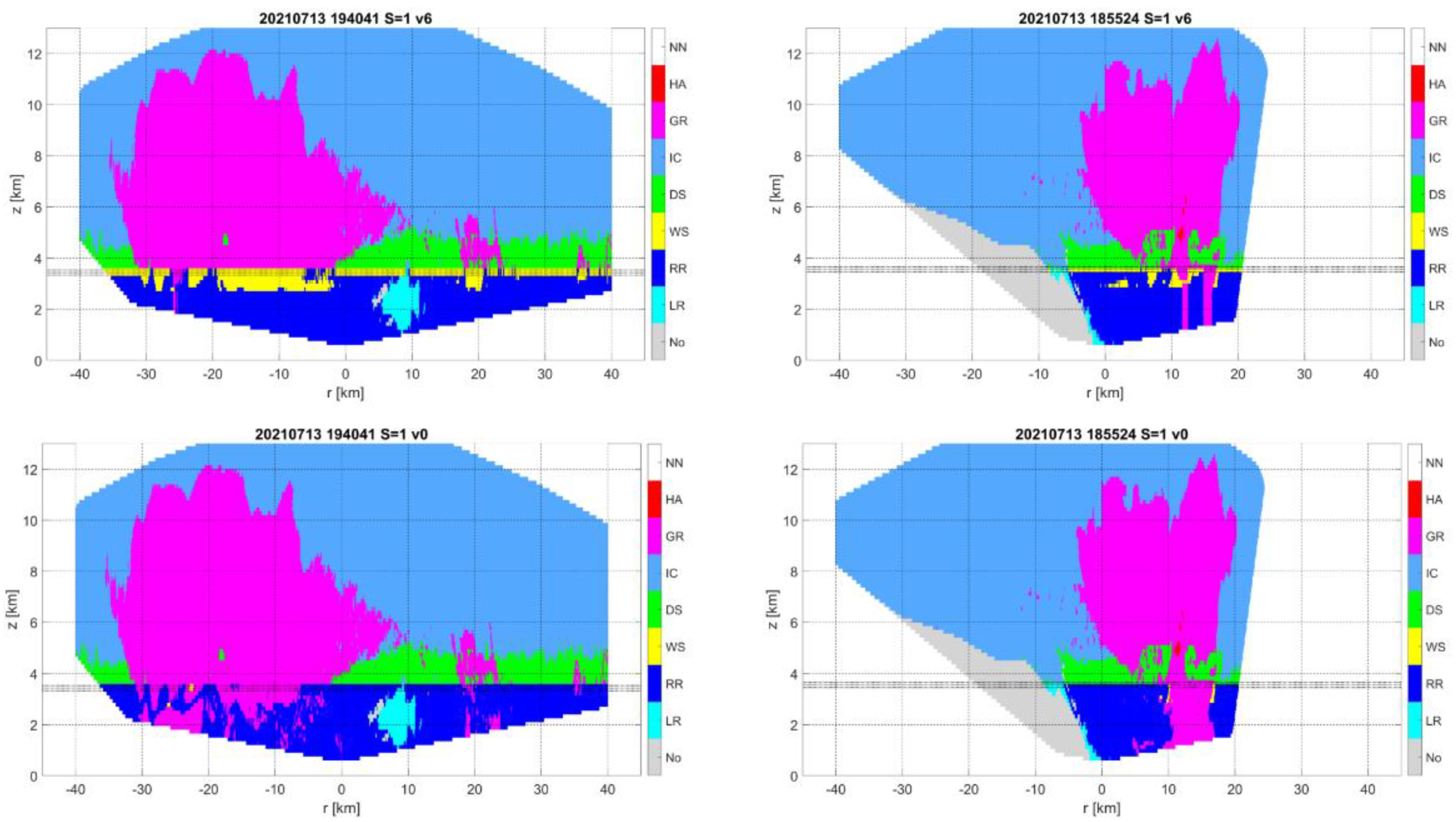
The first three conditions were also applied in [21]. The impact of the fourth and the fifth conditions is illustrated in Figure 2 together with the application of qsiclass. The difference between the original classification [21] and our XCLASS is mainly that the original one gives very little wet snow. In contrast, XCLASS reduces graupel and hail below ML and replaces them with rain. We cannot objectively validate these results; nevertheless, subjectively, we consider them more likely. In particular, the original method seems to generally overestimate the occurrence of near-ground graupel and hail below the ML, which is not confirmed by ground-based observations.
The functions FTiclass and the height of the ML depend on T, which is difficult to determine accurately, especially in convective storms. The height of the ML can be estimated by measurements of Doppler polarimetric radars. Despite that, we chose a simpler method, making use of the current temperature measurements available at the Milešovka observatory, and applied a standard vertical temperature gradient, i.e., the decrease of 6.5 °C per 1 km of altitude, on the measurements. The reason for using this simple method is that our research is focused on severe summer convective storms and we are mainly interested in cloud areas at very high altitudes; therefore, determining the exact height of the ML is not crucial for us. We are aware that the chosen procedure has evident shortcomings; however, the estimation of temperature is difficult and we have left more thorough estimation of T for future study.
In the final step, we distinguished rain based on Zh value (Zh < 10 dBZ), which we call light rain in this paper, from rain (Zh ≥ 10 dBZ) in places where the rain was identified, and we identify graupel (Zh < 50 dBZ) and hail (Zh ≥ 50 dBZ). The threshold values of Zh were selected subjectively. For instance, in the case of hail, we deliberately chose a lower value than the usual 55 dBZ, e.g., [22], because our experience has shown that the FURUNO radar rarely gives values above 55 dBZ in vertical scanning, probably due to partial attenuation.
We calculated Zh in a constant altitude PPI level of 2 km (CAPPI 2km). The value for a given point of the CAPPI 2km was set to the value measured in the nearest PPI level and the resulting field was smoothed using a median filter applied to 3 by 3 radar pixels.
2.3. Satellite Data Meteosat Second Generation
In this study, we used satellite data measured by geostationary satellites Meteosat Second Generation (MSG-9, -10 and -11), which are operated by EUMETSAT (European Organisation for the Exploitation of Meteorological Satellites) and located at geostationary orbit (approximately 36,000 km above the Earth’s surface). Specifically, we used data from the Spinning Enhanced Visible and Infrared Imager (SEVIRI) sensor on the board MSG, recognized as a useful tool for monitoring dynamical and microphysical properties of developing storms, cloud-top temperature, cloud-top cooling rate, etc.
In this paper, we focused on: (i) the brightness temperature (BT) in the infrared channel with a wavelength of 10.8 μm (IR10.8), (ii) the water vapor channel with a wavelength of 6.2 μm (WV6.2), and (iii) their difference (BTD = WV6.2 − IR10.8). The BT observed in IR10.8 measures thermal radiation emitted by the surface in the case of clear-sky conditions, or by clouds. This means that the BT in IR10.8 is directly related to cloud top temperatures if a cloud is present at a given place. WV6.2 is used for interpretation of water vapor content in high tropospheric layers.
Based on BTD values, it is possible to estimate whether there is an overshooting top (OT) in the monitored storm or not. OT is a domelike protrusion above a cumulonimbus anvil, which is caused by a strong updraft through its equilibrium level near tropopause. OT indicates the existence of a deep convective storm with an updraft of sufficient strength to penetrate through the tropopause into the lower stratosphere. Existence of OT is often associated with severe weather, such as heavy rainfall, damaging winds, large hail, lightning, and serious turbulence which endangers air safety. When an updraft is strong enough to penetrate through the tropopause, the penetrating warmer and moister air adds additional radiance in the WV6.2 to the thermal emission originating from the cold storm top, but remains transparent to the IR10.8. Therefore, BTD gains positive values, which indicate the presence of a deep convective storm, e.g., [23,24,25]. There are more effective but also more demanding methods recognizing the existence of OTs [24]. We used BTD in this paper as an indicator of severe convective storms.
The reason for using the above-described satellite data is that they supplement the radar information well for the case of convective events and they also provide data which can be used for validation of our radar data. Other satellite data do not provide fundamentally new information about the development of the studied storms, which is why we did not use them in this study. In addition, we have experience with using these data [5,26].
It should be mentioned that the horizontal resolution of the satellite data for the considered region is approximately 5 km in both south-north and west-east directions. Their relatively low resolution is their main disadvantage. We corrected the measured satellite data using parallax correction, which also can contribute to a decrease in the horizontal accuracy of the data.
However, despite the described shortcomings, the use of MSG data is important in our analysis because it enables validation of vertical radar scans. Specifically, it provides the opportunity to test whether the radar data correctly identify cloud tops.
2.4. Lightning Data and Other Complementary Data
We used lightning data as complementary data to illustrate the strength of convective events in this study. Specifically, we used lightning discharges from the EUCLID (European Cooperation for Lightning Detection) network provided by the BLIDS service (Blitz Informationsdienst von Siemens) [27]. We collected data from around the Milešovka observatory up to a distance of 100 km and we calculated the number of discharges recorded in 1-min intervals up to 1.5 and 5 km from the observatory. We did not distinguish cloud-to-cloud from cloud-to-ground strokes. Cloud-to-cloud strokes represented about 90% of the total strokes in our dataset.
To identify storm existence above the Milešovka observatory, we used a standard set of synoptic data measured at the observatory available every 10 min. We used temperature, wind characteristics (actual, mean and maximum wind speed and direction), surface pressure, relative humidity, and precipitation.
3. Results
We studied two convective events, which occurred in 2021 close to the Milešovka observatory. During both cases (29 June and 13 July), lightning activity was observed close to the observatory within 1.5 km.
3.1. 29 June 2021
A cut-off low over France on 29 June 2021 pushed warm, moist, and thus unstable air mass towards Central Europe. A convective environment with CAPE slightly exceeding 1000 J/kg and a moderate 0–6 km wind shear of about 13 m/s was suitable for the development of convective storms.
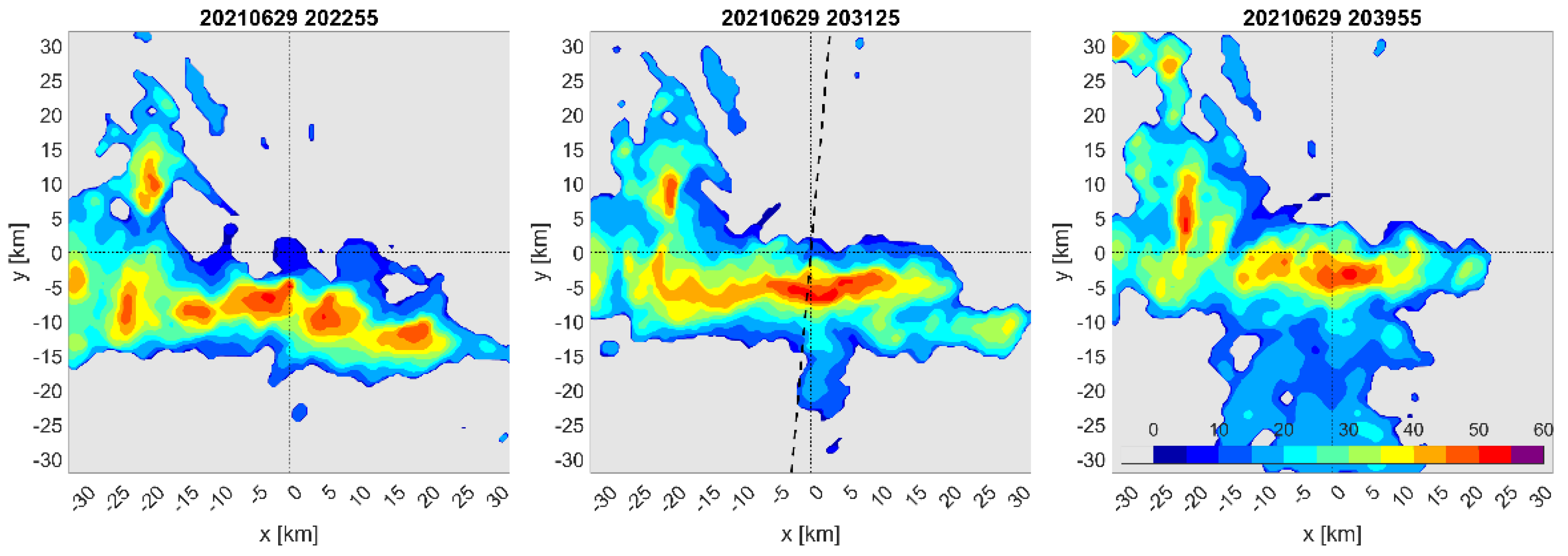
On June 29, in the evening, convective storms, which were accompanied by precipitation and lightning, passed around the Milešovka mountain and partly over its top. The development of storms is documented by the time sequence of CAPPI 2 km radar reflectivity in Figure 3, starting at about 20:22:55 UTC, with a time step of approximately 8.5 min among subfigures. These three subfigures show a well-developed squall line in the southwest of the Milešovka mountain, which moved towards Milešovka, and at the same time, turned in the west-east direction. The squall line consisted of several storms that developed in time. The storms reached their maximum reflectivity at CAPPI 2km at about 20:30 to 20:40 UTC in the immediate vicinity of Milešovka, to the south.
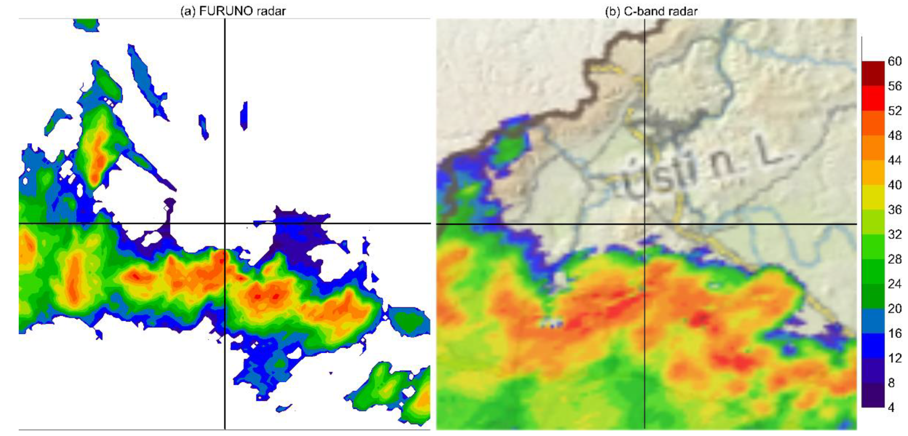
Figure 4 compares measurements of the FURUNO radar and the operational C-band weather radar operated by the Czech Hydrometeorological Institute at 20:20 UTC on 29 June. The operational C-band radar is located at about 100 km south of the FURUNO radar and its horizontal resolution is 1 km. Although the same time is depicted, the projection of shown data and colours of contour levels slightly differ. To enable simple comparisons of radar images, crossed lines indicating the corresponding directions are shown. The position of the FURUNO radar is located at the intersection of the lines.
Figure 4 also depicts the radar reflectivity when significant convective precipitation was recorded in the belt south of the FURUNO radar. It is obvious that this belt caused significant attenuation of the FURUNO radar reflectivity and, compared to the C-band radar, this radar did not show any precipitation beyond the belt. Note that the application of attenuation correction (1) did not significantly improve the FURUNO data.
In Figure 4, the maximum reflectivity measured by both radars is in the range of 52–56 dBZ. The basic structure of the precipitation band is similar for both radars, although it differs in detail. In general, the FURUNO radar gives a more detailed reflectivity structure, which is due to its higher resolution and smaller target spacing compared to the C-band radar, although the sensitivity of the FURUNO radar is lower. It is worth noting that there are different radar outputs in the northwest direction from the Milešovka observatory. The FURUNO radar gives reflectivity below 4 dBZ, while the C-band radar gives reflectivity higher than 8 dBZ. This is a very orographic area situated in the foothills of the Krušné hory (Erzgebirge) mountains with very steep slopes going up to the mountain ridge, which is about 1000 m high.
Comparisons between the data of the two radars yielded similar results, in the case of the second studied event also, i.e., on 13 July 2021 (not shown). They showed that the FURUNO radar gives valuable data in the horizontal plane for convective storms located near the radar, but that the areas behind the storms in the direction away from the radar are strongly affected by attenuation, which is a typical feature of X-band weather radars. The application of attenuation correction is not very helpful in such cases. The FURUNO radar gives similar values of the maximum reflectivity to those of the operational C-band radar in places where measurements are not attenuated. As compared to the operational C-band radar fields, the FURUNO radar fields contain more detailed structures due to the higher horizontal resolution of the radar. Based on FURUNO and C-band radar comparison, we can conclude that FURUNO radar data for convective storms which occur close to the radar site are suitable for the analysis of storms since they are not significantly affected by higher values of the beam width and lower values of sensitivity parameters of the radar.
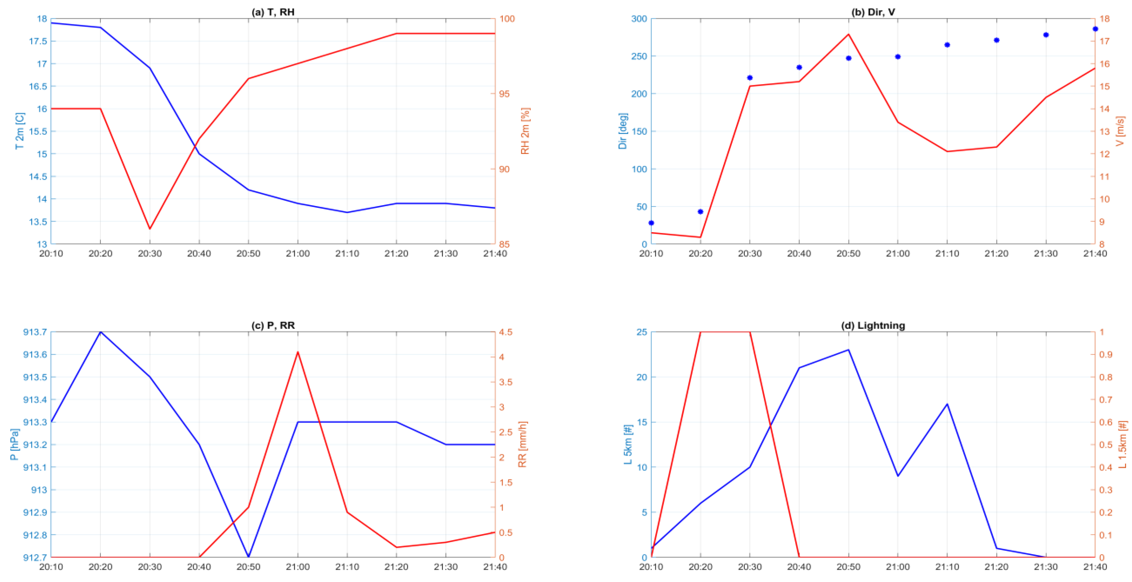
The time evolution of standard measured meteorological quantities is shown in Figure 5. At 20:20 UTC, the temperature began to drop significantly. By that time, there was also a significant change in wind direction. Significant increases in current and maximum wind speeds were recorded after 20:20 UTC. From this time onwards, the wind had significant western and south-western components, which agrees with Figure 3. Although the wind characteristics measured at the Milešovka observatory were similar to wind characteristics in the free atmosphere due to the conical shape of the mountain and the location of the wind measurements on the top of the tower (Figure 1), it was not possible to deduce the wind direction and speed in the upper atmosphere. Apparent changes in the values of temperature, wind characteristics, and other quantities confirm that convective storms began to affect the weather at the Milešovka observatory at about 20:20 UTC (Figure 5).
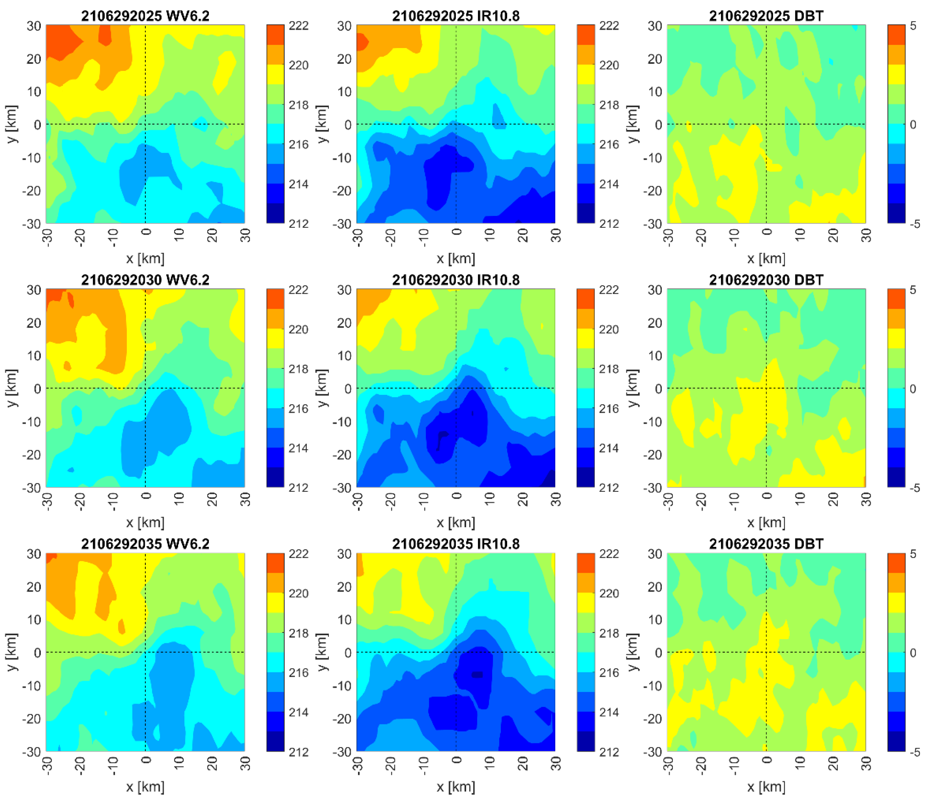
Measurements of MSG provide an overhead view of the development of clouds and convective storms. The measured values of IR10.8, shown in Figure 6, correspond to the BTs of the cloud tops, which characterize vertical cloud extent, and is related to the intensity of convection. On all dates shown, the lowest temperature was around 213 K and near Milešovka. Sounding measurements from midnight at Praha-Libuš station, which is about 70 km away from the Milešovka, indicated that the IR10.8 temperature corresponds to an altitude of about 12 km. BTD values were between 2 and 3 °C in the wider surroundings of Milešovka. Therefore, strong convection and OTs were likely to occur in this area.
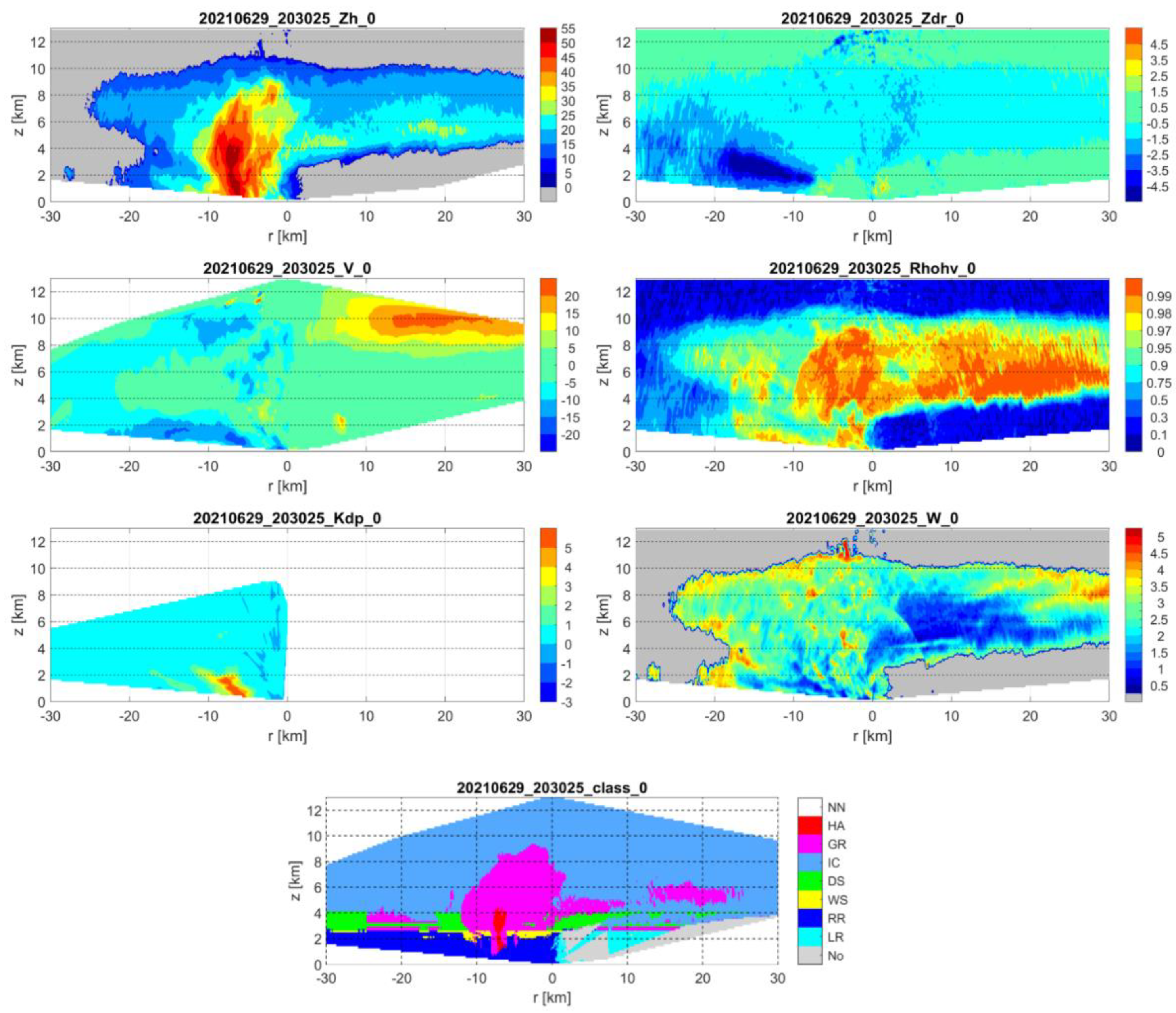
Figure 7 contains vertical cross sections (RHI scans) measured by FURUNO radar. It shows Zh [dBZ], Zdr [dBZ], V [m/s] and Rhohv [–]. The Zh, Zdr and Rhohv are depicted because their values are crucial for hydrometeor classification (Section 2). Figure 7 also shows results of the hydrometeor classification performed by the XCLASS algorithm described in Section 2.2. Note that the cross section is oriented from the south to the north (see Figure 3).
Figure 7 shows the structure of the storm at the time when its activity was at its peak. Fields of Zh show a typical structure of a convective storm moving along the horizontal axis. In our case, it goes southwest from the Milešovka and the radar image is created by projecting the storm into the plane of the cross section, which approximately corresponds to the direction of the storm motion. This is also confirmed by radial velocities, which are influenced by the terminal velocities of hydrometeors, though it can be roughly stated that they have negative values to the left of Milešovka and positive values to the right of Milešovka. The wind speed in the upper part of the storm exceeds the storm speed, creating the well-known anvil before the storm in the direction of its movement.
The core of the storm is located about 7 km south of the radar and the cloud top is about 11 km, with a ridge extending up to 12 km above the central part of the storm. Consistent with satellite measurements, it may be an OT. The distinct change in sign of the V values below the probable OT and the high W values confirm the existence of turbulence and rotational motions of the hydrometeors in this area, which is consistent with the formation of an OT. In the core of the storm, the maximum Zh value exceeded 55 dBZ at the ground and the values above 50 dBZ reached a height of 4 km.
V significantly exceeded 20 m/s at a height of 10 km and at a distance of 15–20 km north of Milešovka. Note that the radial velocity above the radar represents vertical velocities which correspond to the difference in air velocity and terminal velocities of hydrometeors.
Zdr values were almost everywhere negative and lower than expected. Only near the ground in the region of maximum reflectivity were they positive, indicating melting hail. There were also positive values at the front of the storm near the radar. High negative Zdr values south of the radar behind the storm core were probably caused by signal attenuation.
The Rhohv values as a whole appear to be low, which may be caused by attenuation. The values of Zh, Zdr and Rhohv indicate that the anvil of the storm consisted mainly of ice crystals and snow. Low values of Rhohv and high values of Zh indicate that the core of the storm contained hail, which is also visible in the Kdp values. High positive Kdp values in the near-surface core suggest large hydrometeors in high concentrations. However, it should be noted that Kdp values are counted only at points that meet certain Φdp conditions. Therefore, the Kdp values do not cover the whole domain.
The XCLASS hydrometeor classification indicates graupel including hail in the central part of the storm, suggesting suitable conditions for cloud electrification. Hail generally does not reach the ground or the lower edge of the field scanned by the radar, which is likely consistent with reality, as no large areas with graupel or hail were reported on the ground during the event. XCLASS shows certain shortcomings. An example is the narrow horizontal strip of DS, which divides the area covered by GR. Note that XCLASS determines one hydrometeor at a given location only, and there are often small differences among the weights of individual hydrometeors. Therefore, local “illogicalities” may arise. A similar problem can be seen to the north of the radar.
3.2. 13 July 2021
The event on July 13 is similar to that which occurred on 29 June. The air flow over central Europe was determined by a low pressure situated above France. CAPE exceeding 1500 J/kg, together with a strong wind shear between the ground and an altitude of 6 km, helped to develop a squall line with a large amount of lightning discharges close to the Milešovka observatory at approximately 19:00 UTC.
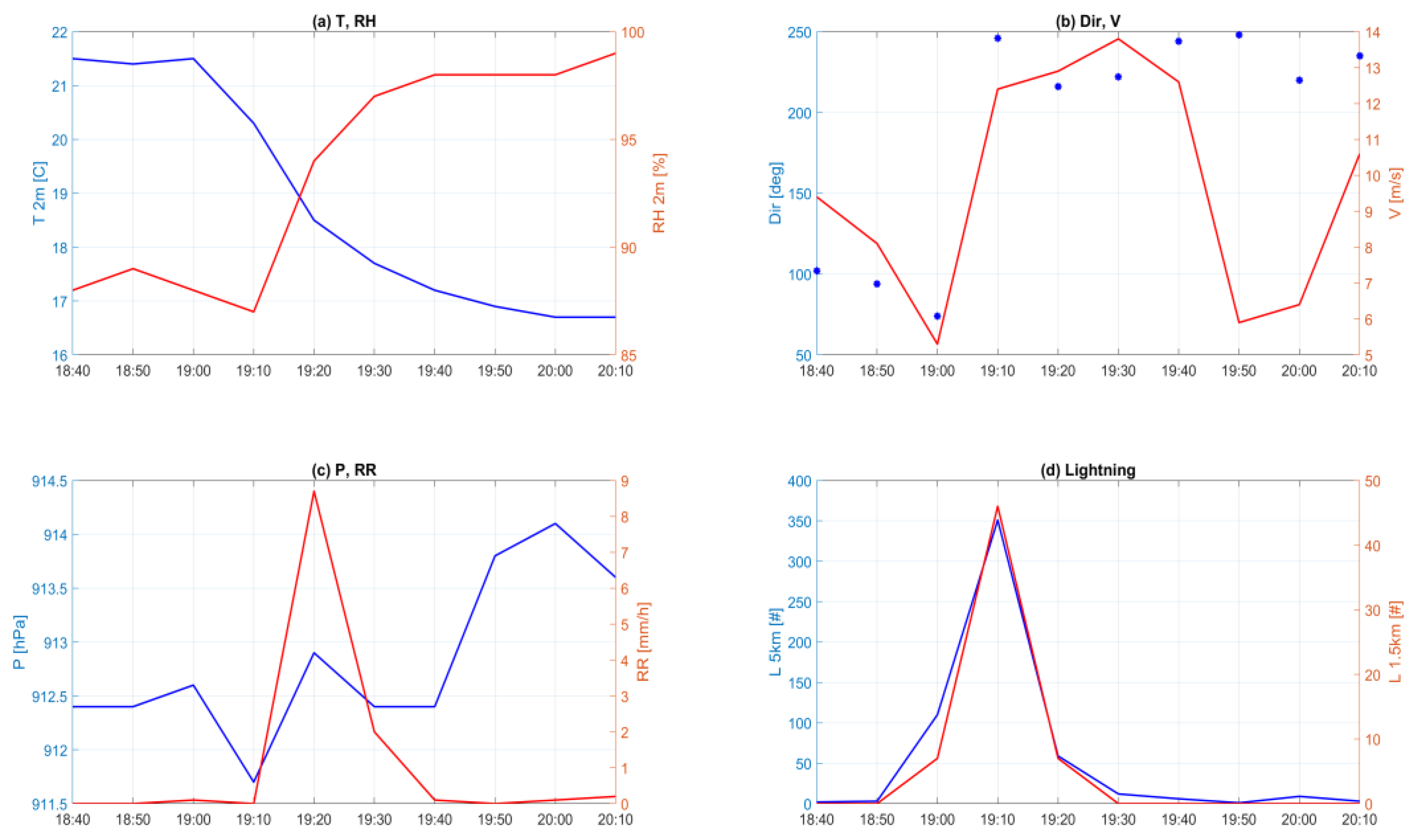
Figure 8 shows ground synoptic data. A big change in wind direction, a sharp drop in temperature, and an obvious increase in humidity indicate the passage of the storm over Milešovka at around 19:10 UTC. This is also confirmed by lightning data. Within 10 min, from 19:00 to 19:10 UTC, 351 lightning flashes were recorded at 5 km and 46 lightning flashes at a distance of 1.5 km from the observatory.
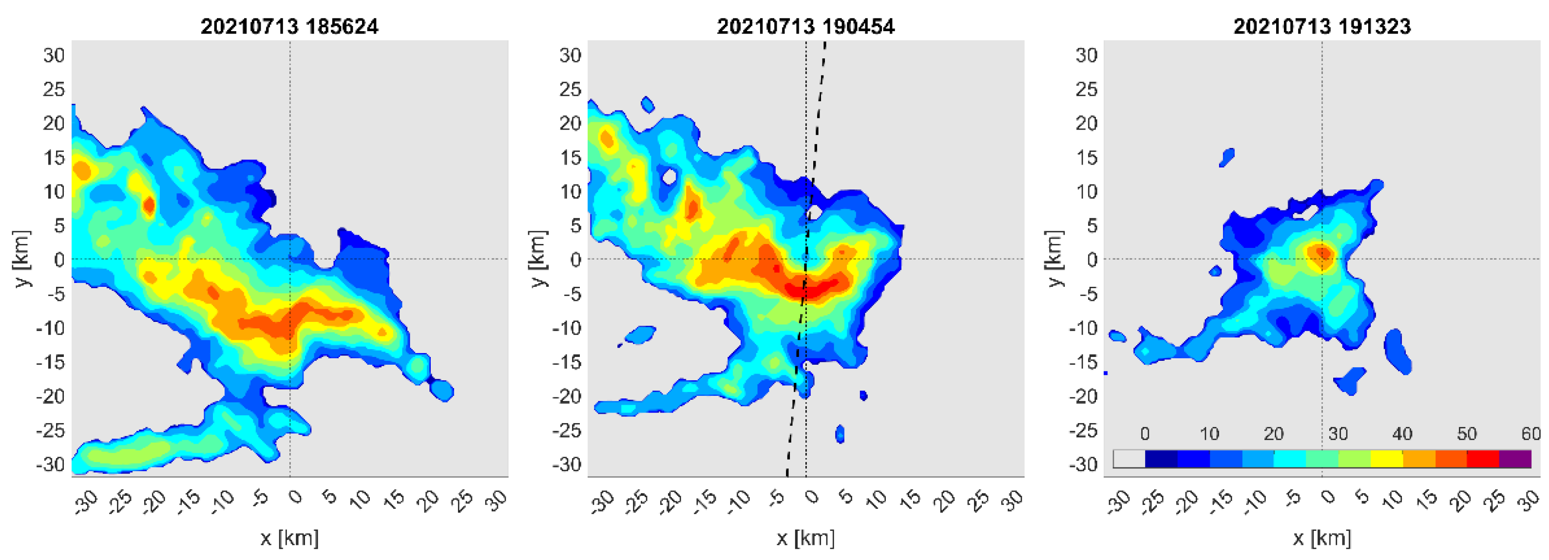
The movement of the squall line and individual storms is shown in Figure 9, which depicts the time evolution of radar reflectivity at CAPPI 2km level with a time step of 8.5 min. As compared to the operational C-band weather radar data (not depicted), there is a noticeable attenuation in the CAPPI 2km data of the FURUNO X-band weather radar in distant areas from the radar site, similar to the event on 29 June. However, the attenuation only very slightly affected the measured storm characteristics near the radar.
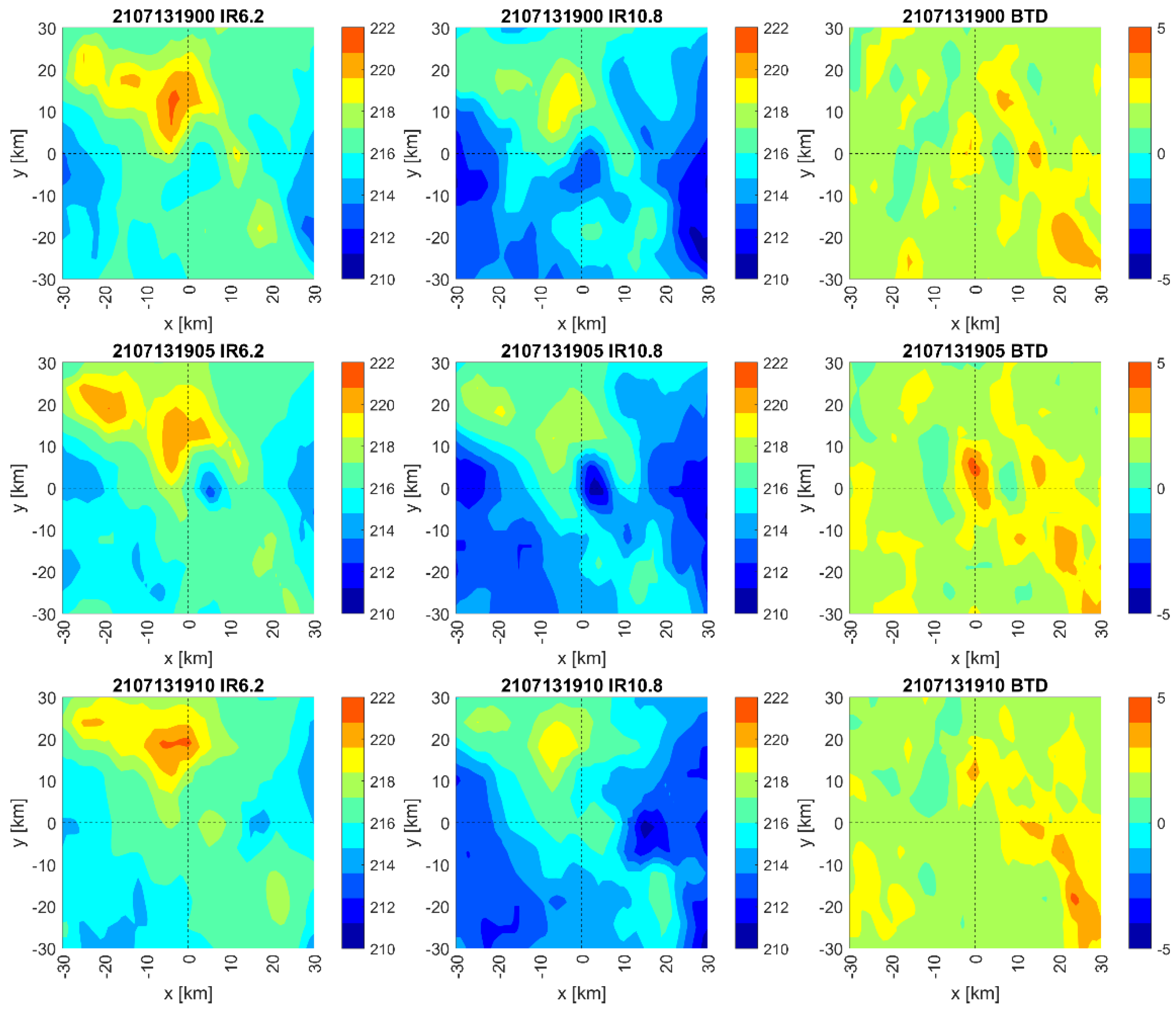
An overhead view of the storm using MSG measurements (Figure 10) corresponds to the movement of the storm identified by the FURUNO radar (Figure 9). The lowest BT values of the channel IR10.8 in the figures shown was between 211 and 212 K. These temperatures corresponded to an altitude of about 17 km, in comparison with the midnight measurement of the Prague-Libuš aerological station. High positive BTD values, whose areal maxima are between 3.8 and 4.5 °C, indicate very strong convection, especially around Milešovka with expected overshooting cloud tops.
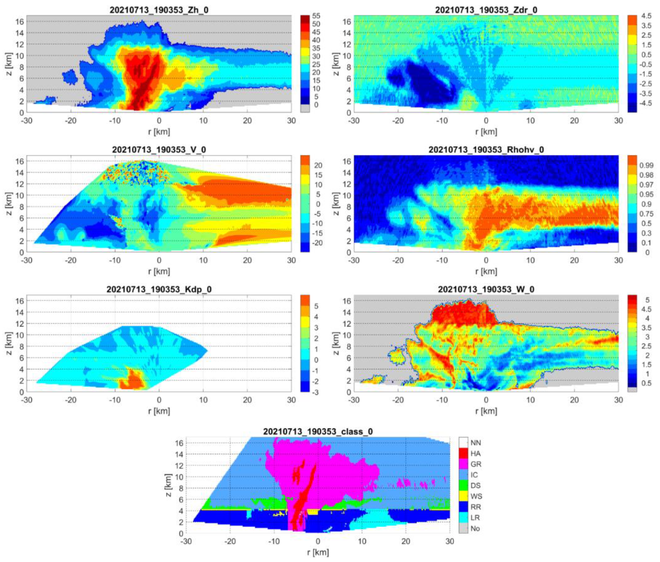
Vertical sections of radar quantities are shown in Figure 11 and the direction of cross-section in Figure 9. They confirm that this is a more intense convective storm than on 29 June. The Zh field shows that the cloud height exceeded 16 km and the storm core, with reflectivity above 50 dBZ, was located from the ground up to 10 km. Zh shows a typical structure of a storm moving along the horizontal axis. The anvil is apparent and confirms the southern component of the storm motion. A rain rate of 8.7 mm precipitation, measured between 19:10 and 19:20, confirms the severity of the storm at Milešovka, although the center of the storm was located further to the south.
The structure of Zdr is similar to that of Figure 7. Very low Zdr values are found at the back of the storm at locations with relatively low reflectivity behind the storm core, with high Zh values in the radar direction. The high Zdr values to the south of the radar at distances greater than 20 km were likely due to attenuation and the attenuation correcting method. Positive Zdr values near the ground in the central part of the storm indicate that either large raindrops or melting water-coated hail were present.
The radial velocity field confirms that the storm is moving approximately from south to north. The largest radial velocity is in the upper half of the anvil, which is moving at speeds above 30 m/s with a maximum of 41 m/s. The Doppler range is approximately ±50 m/s. The displayed radial velocity consists of horizontal and vertical components and the high radial velocities were caused mainly by the horizontal wind component because this area was far from the center of the storm and the vertical velocity could not be great.
It is worth noting local changes in the sign of radial velocities in the upper part of the storm at heights of 12–16 km. These sign changes cannot be attributed to aliasing because the velocities are not so great. The Doppler velocity is calculated from the frequency shift and therefore should not be affected by attenuation. A similar feature of the radial velocity field was also exhibited at other storm times. Therefore, we believe that the measurements indicate significant turbulence in the upper part of the storm, leading to rotational air motions in this region [28]. The large variability in radial velocities in this region is confirmed by W.
The Rhohv reached values of 0.8 to 0.99 in the central part of the storm. The low values at the southern edge of the storm are probably due to attenuation. In areas where there is no attenuation, Rhohv values are greater than 0.99. The Kdp field has a very similar structure to that of the 29 June storm. The high positive values in the near-surface region in the central part of the storm indicate the existence of melting hail.
The XCLASS algorithm determined that the core of the storm contained graupel and hail, which reached vertically up to the heights of 10 km. The classification algorithm also confirmed that this storm was stronger than the storm on 29 June and the distribution of hydrometeors to be reasonable.
4. Discussion
The FURUNO X-band radar is located on the tower of the Milešovka observatory (Figure 1), the sole place with an unobstructed view of the surroundings. Measured data were of good quality except for those measured at higher elevations (above 20°) and close to the radar site (up to 1.5 km), where artefacts sometimes appeared. These artefacts were mainly manifested in vertical scans and cannot be removed by standard procedures used in radar data control because it is not clear what specifically causes them. Interestingly, they did not appear when there was low cloud cover over the radar. We are currently working on eliminating these problems in cooperation with the radar manufacturer. However, it should be noted that the possible artefacts lowering the data quality in the vicinity of the radar did not affect the presented results and should also not burden the use of the radar in the planned investigation of cloud microphysics in the mid and upper troposphere.
Analysis of the measured radar data confirmed that significant attenuation could occur in X-band radar reflectivity measurements and that the radar did not see precipitation beyond the heavy precipitation area when displaying reflectivity using CAPPI 2km fields. The attenuation was also evident in the vertical scans, which are crucial for showing the internal structure of the storms. Even when Zdr correction was applied, the measured Zdr were generally lower than expected, and the Zdr values were difficult to explain in some locations (e.g., Figure 11, for r < −20 km). Other attenuation correction methods than the manufacturer proposed will need to be tested. The attenuation and noise problems probably cause abnormally low Rhohv values in some areas of the scan. Attenuation correction has not been applied to the Rhohv calculation but will be necessary. We plan to apply the method given by Ryzhkov and Zrnić [18]. The attenuation and noise problems cause Kdp values to be calculated only in a part of the region. This calculation is directly built into the radar software and cannot be easily changed. Despite these shortcomings, the measured RHI scans show the structure of the storms, albeit the measured values need to be interpreted carefully. It should be emphasized that the storm of 13 July, in particular, was an extreme storm that occurs very rarely in the area of Milešovka.
Interesting radial velocities were measured on 13 July. These are different radial velocity orientations in the upper part of the cloud above the storm core at altitudes of 12–16 km. We believe that these data indicate strong turbulence and rotating air motions in the top of the cloud above the tropopause.
Comparing the measured radar and satellite data, there is a good agreement in the determined cloud top heights. Satellite data indicate suitable conditions for the formation of OT in the area near Milešovka. The radar data also confirms the existence of OT, namely the structures of the Zh and V fields.
The important result of this study is the developed XCLASS algorithm, classifying hydrometeors based on radar polarimetric data inspired by [21]. We found that the original algorithm gave unrealistic results around and below the melting layer. Thus, in XCLASS, we changed the values of weights of each hydrometeor dependent on values of the measured polarimetric quantities and we expanded the number of values of the measured data, with more hydrometeor types having non-zero weights. This is particularly relevant for the classification of ice and graupel and it also reduces the strictly rectangular shapes of the hydrometeor regions, which certainly better corresponds to reality. In addition, we increased the weight of wet snow in the ML and introduced the condition that if there is dry snow above the ML, then there is wet snow in the ML. Further, we introduced the condition that no graupel/hail can be formed below the ML unless there is graupel/hail above the ML. The original algorithm gave wet snow very rarely and, on the contrary, existence of graupel/hail below the ML was frequent, creating isolated graupel/hail areas in the rain area, which is not possible. Moreover, we added the distinction of light rain from rain and distinguished graupel from hail based on radar reflectivity thresholds of the classification algorithm. Although we could not objectively verify the results of our XCLASS algorithm, we subjectively found that it better matched our knowledge of hydrometeor occurrence in storms.
5. Conclusions
The analysis of two severe convective storms, which occurred in 2021, confirmed that the newly installed FURUNO X-band weather radar on the top of the tower at the Milešovka observatory is suitable for the research of convection in the mid and upper troposphere by means of RHI scans.
The basic conclusions are:
- The attenuation of X-band radar measurements is noticeable in PPI scans and partly in RHI scans. The attenuation is visible even when the attenuation correction is applied to Zh and Zdr. Attenuation is also visible in Rhohv, where the correction has not yet been applied. The results show that the attenuation correction should be considered;
- Although the radar measurements are contaminated by attenuation, they give information about the cloud structure. However, the measurements should be interpreted with caution;
- Radial velocity measurements indicate a strongly turbulent character of the flow in the upper part of the plume. This is particularly evident in the extreme storm of 13 July 2021;
- Radar measurements of the upper part of the cloud cover are consistent with the data measured by the Meteosat Second Generation satellite;
- The hydrometeor classification algorithm that we call XCLASS, developed by modifying a previously published procedure, to a large extent removes the shortcomings of the original algorithm and, subjectively, gives more acceptable results;
- Analysis of two convective storms showed several erroneous measurements occurring near and above the radar. This problem is being addressed; however, it does not affect the results and the use of radar data for convective cloud research.
We plan to continue our research on convective storms using radar data. Specifically, we will focus on more precise estimation of the ML height using radar data. Then we will deal with comparisons of the measured data by the X-band FURUNO radar and Ka-band cloud profiler, which is also located at the Milešovka station.
Author Contributions
G.B. conceived the paper and processed and interpreted satellite data; Z.S. conceived the paper and processed and interpreted radar data; J.P. verified the results, reviewed and edited the manuscript; O.F. provided consultancy assistance in the interpretation of radar data; P.Z. performed meteorological analyses. All authors have read and agreed to the published version of the manuscript.
Funding
This research was funded by project CRREAT (reg. number: CZ.02.1.01/0.0/0.0/15_003/0000481) call number 02_15_003 of the Operational Programme Research, Development, and Education.
Data Availability Statement
The data used in the research are available from the authors upon request.
Acknowledgments
The research was also supported by Charles University (UNCE/HUM 018) and by project Strategy AV21, Water for Life. Figure 4b was kindly provided by the Czech Hydrometeorological Institute. The authors would like to thank three anonymous referees for their comments that contributed significantly to the improvement of the paper.
Conflicts of Interest
The authors declare no conflict of interest.
Appendix A. We Present here all Parameter Values Needed for the Application of XCLASS Algorithm

Table A1.
The parameters T1, T2, T3, and T4 of the trapezoidal function FTiclass (T) dependent on hydrometeor type.
Table A1.
The parameters T1, T2, T3, and T4 of the trapezoidal function FTiclass (T) dependent on hydrometeor type.
| Hydrometeor | T1 | T2 | T3 | T4 |
|---|---|---|---|---|
| Rain | −4 | −0.5 | 50 | 50 |
| Wet snow | −5 | −2.0 | 4 | 7 |
| Dry snow | −15 | −10.0 | 0 | 3 |
| Ice | −75 | −70.0 | −10 | −3 |
| Graupel/Hail | −90 | −20.0 | 20 | 40 |
Table A2.
2D table used for calculation of weight for occurrence of a given hydrometeor based on condition that the radar measured Zh and Kdp. The left column contains Zh values (upper boundary is not used). The columns R1, R2, W1, W2, S1, S2, I1, I2, H1, and H2 contain parameters for the construction of a trapezoidal function FTiclass for rain (R1, R2), for wet snow (W1, W2), dry snow (S1, S2), ice (I1, I2), and hail (H1, H2), which are used to calculate weights of individual hydrometeors.
| Zh [dBZ] | R1 | R2 | W1 | W2 | S1 | S2 | I1 | I2 | H1 | H2 |
|---|---|---|---|---|---|---|---|---|---|---|
| 0–2.5 | −0.66 | 0.22 | - | - | - | - | - | - | - | - |
| 2.5–5 | −0.66 | 0.22 | - | - | - | - | −0.44 | 0.66 | - | - |
| 5–7.5 | −0.66 | 0.22 | - | - | - | - | −0.66 | 0.66 | - | - |
| 7.5–10 | −0.66 | 0.22 | - | - | - | - | −0.66 | 0.66 | - | - |
| 10–12.5 | −0.66 | 0.22 | - | - | - | - | −0.66 | 0.66 | - | - |
| 12.5–15 | −0.66 | 0.22 | - | - | - | - | −0.66 | 0.66 | - | - |
| 15–17.5 | −0.66 | 0.22 | - | - | 0.22 | 0.22 | −0.66 | 0.66 | - | - |
| 17.5–20 | −0.66 | 0.22 | - | - | −0.22 | 0.66 | −0.66 | 0.66 | - | - |
| 20–22.5 | −0.66 | 0.22 | 0.88 | 1.10 | −0.44 | 0.88 | −0.44 | 0.66 | - | - |
| 22.5–25 | −0.66 | 0.22 | 0.22 | 1.32 | −0.44 | 0.44 | −0.44 | 0.44 | - | - |
| 25–27.5 | −0.66 | 0.22 | 0.22 | 1.32 | −0.44 | 0.88 | - | - | - | - |
| 27.5–30 | −0.66 | 0.22 | 0.22 | 1.32 | −0.44 | 0.88 | - | - | - | - |
| 30–32.5 | −0.44 | 0.22 | 0.22 | 1.32 | −0.44 | 0.88 | - | - | - | - |
| 32.5–35 | −0.44 | 0.44 | 0.22 | 1.32 | −0.44 | 0.88 | - | - | - | - |
| 35–37.5 | −0.44 | 0.44 | 0.22 | 1.32 | −0.44 | 0.88 | - | - | - | - |
| 37.5–40 | −0.44 | 0.44 | 0.22 | 1.32 | −0.44 | 0.88 | - | - | - | - |
| 40–42.5 | −0.44 | 0.44 | 0.22 | 1.32 | −0.44 | 0.88 | - | - | - | - |
| 42.5–45 | −0.44 | 0.66 | 0.22 | 1.32 | −0.22 | 0.66 | - | - | - | - |
| 45–47.5 | −0.22 | 0.88 | 0.22 | 1.32 | - | - | - | - | - | - |
| 47.5–50 | 0.00 | 1.32 | 0.44 | 1.32 | - | - | - | - | −0.66 | 2.86 |
| 50–52.5 | 0.44 | 2.20 | - | - | - | - | - | - | −0.66 | 3.08 |
| 52.5–55 | 1.32 | 3.30 | - | - | - | - | - | - | −0.66 | 3.30 |
| 55–57.5 | 3.08 | 5.28 | - | - | - | - | - | - | −0.66 | 3.52 |
| 57.5–60 | 4.62 | 5.28 | - | - | - | - | - | - | −0.66 | 3.74 |
| 60–62.5 | - | - | - | - | - | - | - | - | −0.66 | 3.74 |
| 62.5–65 | - | - | - | - | - | - | - | - | −0.66 | 3.96 |
| 65–67.5 | - | - | - | - | - | - | - | - | −0.66 | 4.18 |
| 67.5–70 | - | - | - | - | - | - | - | - | −0.66 | 4.40 |
| 70–99 | - | - | - | - | - | - | - | - | −0.66 | 4.62 |
Table A3.
The same as Table A2 but for Rhohv.
Table A3.
The same as Table A2 but for Rhohv.
| Zh [dBZ] | R1 | R2 | W1 | W2 | S1 | S2 | I1 | I2 | H1 | H2 |
|---|---|---|---|---|---|---|---|---|---|---|
| 0–2.5 | 0.97 | 1.00 | - | - | - | - | - | - | - | - |
| 2.5–5 | 0.97 | 1.00 | - | - | - | - | - | - | - | - |
| 5–7.5 | 0.97 | 1.00 | - | - | - | - | 0.92 | 0.99 | - | - |
| 7.5–10 | 0.97 | 1.00 | - | - | - | - | 0.92 | 0.99 | - | - |
| 10–12.5 | 0.97 | 1.00 | - | - | - | - | 0.92 | 0.99 | - | - |
| 12.5–15 | 0.97 | 1.00 | - | - | - | - | 0.92 | 0.99 | - | - |
| 15–17.5 | 0.97 | 1.00 | - | - | 0.96 | 0.97 | 0.92 | 0.99 | - | - |
| 17.5–20 | 0.97 | 1.00 | - | - | 0.93 | 0.99 | 0.92 | 0.99 | - | - |
| 20–22.5 | 0.97 | 1.00 | 0.89 | 0.92 | 0.92 | 0.99 | 0.93 | 0.99 | - | - |
| 22.5–25 | 0.97 | 1.00 | 0.86 | 0.96 | 0.92 | 0.99 | 0.94 | 0.98 | - | - |
| 25–27.5 | 0.97 | 1.00 | 0.86 | 0.96 | 0.92 | 0.99 | - | - | - | - |
| 27.5–30 | 0.96 | 1.00 | 0.86 | 0.96 | 0.92 | 0.99 | - | - | - | - |
| 30–32.5 | 0.96 | 1.00 | 0.86 | 0.96 | 0.92 | 0.99 | - | - | - | - |
| 32.5–35 | 0.95 | 1.00 | 0.86 | 0.96 | 0.92 | 0.99 | - | - | - | - |
| 35–37.5 | 0.95 | 1.00 | 0.86 | 0.96 | 0.92 | 0.99 | - | - | - | - |
| 37.5–40 | 0.95 | 1.00 | 0.86 | 0.96 | 0.92 | 0.99 | - | - | - | - |
| 40–42.5 | 0.95 | 1.00 | 0.86 | 0.96 | 0.92 | 0.99 | - | - | - | - |
| 42.5–45 | 0.95 | 1.00 | 0.86 | 0.96 | 0.93 | 0.99 | - | - | - | - |
| 45–47.5 | 0.95 | 1.00 | 0.86 | 0.96 | - | - | - | - | - | - |
| 47.5–50 | 0.94 | 1.00 | 0.88 | 0.95 | - | - | - | - | 0.80 | 1.00 |
| 50–52.5 | 0.94 | 1.00 | - | - | - | - | - | - | 0.80 | 1.00 |
| 52.5–55 | 0.94 | 1.00 | - | - | - | - | - | - | 0.80 | 1.00 |
| 55–57.5 | 0.94 | 1.00 | - | - | - | - | - | - | 0.80 | 1.00 |
| 57.5–60 | 0.94 | 1.00 | - | - | - | - | - | - | 0.80 | 1.00 |
| 60–62.5 | 0.94 | 1.00 | - | - | - | - | - | - | 0.80 | 1.00 |
| 62.5–65 | 0.94 | 1.00 | - | - | - | - | - | - | 0.80 | 1.00 |
| 65–67.5 | 0.95 | 1.00 | - | - | - | - | - | - | 0.80 | 1.00 |
| 67.5–70 | 0.96 | 1.00 | - | - | - | - | - | - | 0.80 | 1.00 |
| 70–99 | 0.96 | 1.00 | - | - | - | - | - | - | 0.80 | 1.00 |
Table A4.
The same as Table A2 but for Zdr.
Table A4.
The same as Table A2 but for Zdr.
| Zh [dBZ] | R1 | R2 | W1 | W2 | S1 | S2 | I1 | I2 | H1 | H2 |
|---|---|---|---|---|---|---|---|---|---|---|
| 0–2.5 | −0.72 | 0.83 | - | - | - | - | - | - | - | - |
| 2.5–5 | −0.72 | 0.83 | - | - | - | - | −0.1 | 0.83 | - | - |
| 5–7.5 | −0.72 | 0.83 | - | - | - | - | −0.1 | 0.83 | - | - |
| 7.5–10 | −0.72 | 0.83 | - | - | - | - | −0.1 | 0.83 | - | - |
| 10–12.5 | −0.72 | 0.83 | - | - | - | - | −0.1 | 0.83 | - | - |
| 12.5–15 | −0.72 | 0.83 | - | - | - | - | −0.1 | 0.83 | - | - |
| 15–17.5 | −0.72 | 0.83 | - | - | 0.21 | 0.21 | −0.1 | 0.83 | - | - |
| 17.5–20 | −0.72 | 1.14 | - | - | −0.41 | 0.52 | −1.34 | 0.52 | - | - |
| 20–22.5 | −0.72 | 1.14 | 1.14 | 2.38 | −0.41 | 0.83 | −1.03 | 0.52 | - | - |
| 22.5–25 | −0.72 | 1.14 | −0.41 | 3 | −0.41 | 0.83 | −1.03 | 0.21 | - | - |
| 25–27.5 | −0.72 | 1.14 | −0.41 | 3 | −0.41 | 0.83 | - | - | - | - |
| 27.5–30 | −0.41 | 1.14 | −0.41 | 3 | −0.41 | 0.83 | - | - | - | - |
| 30–32.5 | −0.41 | 1.45 | −0.41 | 3 | −0.41 | 0.83 | - | - | - | - |
| 32.5–35 | −0.41 | 1.45 | −0.41 | 3 | −0.41 | 0.83 | - | - | - | - |
| 35–37.5 | −0.1 | 1.45 | −0.41 | 3 | −0.41 | 0.83 | - | - | - | - |
| 37.5–40 | −0.1 | 1.76 | −0.41 | 3 | −0.41 | 0.83 | - | - | - | - |
| 40–42.5 | 0.21 | 1.76 | −0.41 | 3 | −0.41 | 0.83 | - | - | - | - |
| 42.5–45 | 0.21 | 2.07 | −0.41 | 3 | −0.41 | 0.52 | - | - | - | - |
| 45–47.5 | 0.52 | 2.07 | −0.1 | 3 | - | - | - | - | - | - |
| 47.5–50 | 0.52 | 2.38 | 0.21 | 2.69 | - | - | - | - | −0.41 | 3 |
| 50–52.5 | 0.83 | 2.69 | - | - | - | - | - | - | −0.41 | 3 |
| 52.5–55 | 1.14 | 2.69 | - | - | - | - | - | - | −0.41 | 3 |
| 55–57.5 | 1.14 | 3 | - | - | - | - | - | - | −0.41 | 3 |
| 57.5–60 | 1.45 | 3 | - | - | - | - | - | - | −0.41 | 3 |
| 60–62.5 | 1.45 | 3 | - | - | - | - | - | - | −0.41 | 2.69 |
| 62.5–65 | 1.76 | 3.31 | - | - | - | - | - | - | −0.41 | 2.38 |
| 65–67.5 | 2.07 | 3.31 | - | - | - | - | - | - | −0.41 | 2.38 |
| 67.5–70 | 2.38 | 3.31 | - | - | - | - | - | - | −0.41 | 2.38 |
| 70–99 | 2.69 | 3.31 | - | - | - | - | - | - | −0.41 | 2.38 |
References
- Brázdil, R.; Chroma, K.; Púčik, T.; Černoch, Z.; Dobrovolný, P.; Dolák, L.; Kotyza, O.; Řezníčková, L.; Taszarek, M. The climatology of significant tornadoes in the Czech Republic. Atmosphere 2020, 11, 689. [Google Scholar] [CrossRef]
- Kašpar, M.; Müller, M.; Kakos, V.; Řezáčová, D.; Sokol, Z. Severe storm in Bavaria, the Czech Republic and Poland on 12–13 July 1984: A statistic- and model-based analysis. Atmos. Res. 2009, 93, 99–110. [Google Scholar] [CrossRef]
- Sokol, Z.; Zacharov, P.; Skripniková, K. Simulation of the storm on 15 August, 2010, using a high resolution COSMO NWP model. Atmos. Res. 2014, 137, 100–111. [Google Scholar] [CrossRef]
- Salek, M.; Brezkova, L.; Novak, P. The use of radar in hydrological modeling in the Czech Republic—Case studies of flash floods. Nat. Hazards Earth Syst. Sci. 2006, 6, 229–236. [Google Scholar] [CrossRef]
- Bliznak, V.; Sokol, Z.; Zacharov, P. Nowcasting of deep convective clouds and heavy precipitation: Comparison study between NWP model simulation and extrapolation. Atmos. Res. 2017, 184, 24–34. [Google Scholar] [CrossRef]
- Orville, R.E.; Maier, M.W.; Mosher, F.R.; Wylie, D.P.; Rust, W.D. The simultaneous display in a severe storm of lightning ground strike locations onto satellite images and radar reflectivity patterns. Bull. Am. Meteorol. Soc. 1981, 62, 1421. [Google Scholar]
- Putsay, M.; Szenyán, I.; Simon, A. Case study of mesoscale convective systems over Hungary on 29 June 2006 with satellite, radar and lightning data. Atmos. Res. 2009, 93, 82–92. [Google Scholar] [CrossRef]
- Matthee, R.; Mecikalski, J.R.; Carey, L.D.; Bitzer, P.M. Quantitative differences between lightning and nonlightning convective Rainfall. Mon. Weather Rev. 2014, 142, 3651–3665. [Google Scholar] [CrossRef]
- Hu, J.; Rosenfeld, D.; Ryzkov, A.; Zhang, P. Synergetic Use of the WSR-88D radars, GOES-R satellites, and lightning networks to study microphysical characteristics of hurricanes. J. Appl. Meteorol. Climatol. 2020, 59, 1051–1068. [Google Scholar] [CrossRef]
- Mulholland, J.P.; Nesbitt, S.W.; Trapp, R.J.; Rasmussen, K.L.; Salio, P.V. Convective storm life cycle and environments near the Sierras de Cordoba, Argentina. Mon. Weather Rev. 2018, 146, 2541–2557. [Google Scholar] [CrossRef]
- Murillo, E.M.; Homeyer, C.R. Severe Hail fall and hailstorm detection using remote sensing observations. J. Appl. Meteorol. Climatol. 2019, 52, 947–970. [Google Scholar] [CrossRef] [PubMed] [Green Version]
- Sandmæl, T.N.; Homeyer, C.R.; Bedka, K.M.; Apke, J.M.; Mecikalski, J.R.; Khlopenkov, K. Evaluating the ability of remote sensing observations to identify significantly severe and potentially tornadic storms. J. Appl. Meteorol. Climatol. 2019, 52, 2569–2590. [Google Scholar] [CrossRef] [PubMed]
- Jones, T.A.; Stensrud, D.; Wicker, L.; Minnis, P.; Palikonda, R. Simultaneous radar and satellite data storm-scale assimilation using an ensemble kalman filter approach for 24 May 2011. Mon. Weather Rev. 2015, 143, 165–194. [Google Scholar] [CrossRef]
- Khan, M.D.; Rabbani, G.; Das, S.; Panda, S.K.; Kabir, A.; Mallik, M.A.K. Physical and dynamical characteristics of thunderstorms over bangladesh based on radar, satellite, upper-air observations, and WRF model simulations. Pure Appl. Geophys. 2021, 178, 3747–3767. [Google Scholar] [CrossRef]
- Manzato, A.; Davolio, S.; Miglietta, M.M.; Puciloa, A.; Setvak, M. 12 September 2012: A supercell outbreak in NE Italy? Atmos. Res. 2015, 153, 98–118. [Google Scholar] [CrossRef]
- Sokol, Z.; Minářová, J.; Novák, P. Classification of hydrometeors using measurements of the Ka-band cloud radar installed at the Milešovka Mountain (Central Europe). Remote Sens. 2018, 10, 1674. [Google Scholar] [CrossRef] [Green Version]
- Sokol, Z.; Popová, J. Differences in cloud radar phase and power in co and cross-channel—indicator of lightning. Remote Sens. 2021, 13, 503. [Google Scholar] [CrossRef]
- Ośródka, K.; Jan Szturc, J. Improvement in algorithms for quality control of weather radar data (RADVOL-QC System). Atmos. Meas. Tech. 2022, 15, 261–277. [Google Scholar] [CrossRef]
- Ryzhkov, A.V.; Zrnić, D.S. Radar Polarimetry for Weather Observations; Springer: Berlin/Heidelberg, Germany, 2019; Volume 486. [Google Scholar]
- Maesaka, T.; Maki, M.; Iwanami, K.; Tsuchiya, S.; Kieda, K.; Hoshi, A. Operational rainfall estimation by X-band MP radar network in Mlit, Japan. In Proceedings of the 35th Conference on Radar Meteorology, Pittsburgh, PA, USA, 26–30 September 2011; p. 11. [Google Scholar]
- Al-Sakka, H.; Boumahmoud, A.A.; Fradon, B.; Frazier, S.J.; Tabary, P. A new fuzzy logic hydrometeor classification scheme applied to the french X-, C-, and S-band polarimetric radars. J. Appl. Meteorol. Climatol. 2013, 52, 2328–2344. [Google Scholar] [CrossRef]
- Geotis, S.G. Some radar measurements of hailstorms. J. Appl. Meteorol. Climatol. 1963, 2, 270–275. [Google Scholar] [CrossRef] [Green Version]
- Schmetz, J.; Tjemkes, S.A.; Gube, M.; Van de Berg, L. Monitoring deep convection and convective overshooting with METEOSAT. Adv. Space Res. 1997, 19, 433–441. [Google Scholar] [CrossRef]
- Setvak, M.; Lindsey, D.T.; Novak, P.; Wang, P.K.; Radova, M.; Kerkmann, J.; Grasso, L.; Su, S.H.; Rabin, R.M.; St’astka, J.; et al. Satellite-observed cold-ring-shaped features atop deep convective clouds. Atmos. Res. 2010, 97, 80–96. [Google Scholar] [CrossRef]
- Bedka, K.M.; Wang, C.; Rogers, R.; Carey, L.D.; Feltz, W.; Kanak, J. Examining deep convective cloud evolution using total lightning, WSR-88D, and GOES-14 super rapid scan datasets. Weather Forecast. 2015, 30, 571–590. [Google Scholar] [CrossRef]
- Bližňák, V.; Sokol, Z. The exploitation of Meteosat Second Generation data for convective storms over the Czech Republic. Atmos. Res. 2012, 103, 60–69. [Google Scholar] [CrossRef]
- Blids, Der Blitz Informationsdienst Von Siemens. Available online: https://new.siemens.com/global/de/produkte/services/blids.html (accessed on 3 August 2021).
- Lane, T.P.; Sharman, R.D.; Clark, T.L.; Hsu, H.-M. An Investigation of turbulence generation mechanisms above deep convection. J. Atmos. Sci. 2003, 60, 1297–1321. [Google Scholar] [CrossRef]
Figure 1.
Geographical location of the observatory Milešovka and FURUNO radar (837 m a.s.l.) in the Czech Republic in Central Europe. Source of the digital terrain map: www.cuzk.cz (accessed on 12 May 2021).
Figure 1.
Geographical location of the observatory Milešovka and FURUNO radar (837 m a.s.l.) in the Czech Republic in Central Europe. Source of the digital terrain map: www.cuzk.cz (accessed on 12 May 2021).

Figure 2.
Comparison of hydrometeor classifications (LR-light rain, RR-rain, WS-wet snow, DS-dry snow, IC-ice, GR-graupel, HA-hail, NN-no data, No-hydrometeor is not recognized) by the original method (v0, [21]) and the upgraded method (v6, XCLASS) for two terms (see figure titles). Titles contain time in the format year, month, day and hour, minute, second. The Milešovka observatory has coordinate r = 0 and z is altitude a.s.l. The three dotted lines indicate ML.

Figure 3.
Radar reflectivity [dBZ] at CAPPI 2km level at different time steps. Titles of the subfigures present time of measurements in the format year, month, day and hour, minute, second. The Milešovka observatory is in the cross section of the two dotted lines. The dashed line shows a cross section line.

Figure 4.
Comparison of measured radar reflectivity CAPPI 2 km by FURUNO X-band radar (a) and C-band radar (b) operated by the Czech Hydrometeorological Institute on 29 June, at 20:20 UTC. The horizontal resolution of the C-band radar is 1 km and the areas of both radars are the same as in Figure 3 (35 km by 35 km).

Figure 5.
Time evolution on 29 June 2021 at time (horizontal axis, HH:MM) at the Milešovka observatory of (a) temperature at 2 m (T, [°C], blue color) and relative humidity at 2 m (RH, [%], red color), (b) actual wind direction (Dir, [°], blue color) and current wind speed (V, [m/s], red color), (c) atmospheric pressure (P, [hPa], blue color) and accumulated precipitation in the last 10 min (RR [mm], red color), and (d) lightning (L 5 km shows the number of lightning strokes 5 km from Milešovka (blue color), while L 1.5 km represents the number of lightning strokes 1.5 km from Milešovka (red color)).

Figure 6.
BTs [K] of WV6.2, IR10.8, and DBT [°C] at different times. Titles contain time in the format year, month, day and hour, minute, second. The Milešovka observatory is in the intersection of the two dashed lines.
Figure 6.
BTs [K] of WV6.2, IR10.8, and DBT [°C] at different times. Titles contain time in the format year, month, day and hour, minute, second. The Milešovka observatory is in the intersection of the two dashed lines.

Figure 7.
Vertical cross sections Zh [dBZ], Zdr [dBZ], V [m/s], Rhohv [–], Kdp [deg/km], and W [m/s]. “c2” for Zh and Zdr indicates that attenuation correction has been applied. The bottom subfigure presents the classification of hydrometeors. Classes in the hydrometeor classification are: No-no targets; LR-light rain; RR-rain; WS-wet snow; DS-dry snow; IC-ice; GR-graupel; HA-hail; and three horizontal lines denotes estimated position of ML. The cross section is oriented proximately from the south to the north (see Figure 3). Titles contain time in the format year, month, day and hour, minute, second. The Milešovka observatory is in r = 0 and vertical axis shows the altitude above the radar.

Figure 8.
Same as Figure 5 but for 13 July 2021.
Figure 8.
Same as Figure 5 but for 13 July 2021.

Figure 9.
Radar reflectivity [dBZ] at CAPPI 2km level at different time steps. Titles of the subfigures contain the time of measurements in the format year, month, day and hour, minute, second. The Milešovka observatory is in the cross section of the two dotted lines. The dashed line shows a cross section line.

Figure 10.
BTs [K] of IR10.8 at different times. Titles contain time in the format year, month, day and hour, minute, second. The Milešovka observatory is in the cross section of the two dashed lines.
Figure 10.
BTs [K] of IR10.8 at different times. Titles contain time in the format year, month, day and hour, minute, second. The Milešovka observatory is in the cross section of the two dashed lines.

Figure 11.
Vertical cross sections Zh [dBZ], Zdr [dBZ], V [m/s], Rhohv [–], Kdp [deg/km], and W [m/s]. “c2” for Zh and Zdr indicates that attenuation correction has been applied. The bottom subfigure presents the classification of hydrometeors. Classes in the hydrometeor classification are: No-no targets; LR-light rain; RR-rain; WS-wet snow; DS-dry snow; IC-ice; GR-graupel; HA-hail; and three horizontal lines denote estimated position of ML. The cross section is oriented proximately from the south to the north (see Figure 3). Titles contain time in the format year, month, day and hour, minute, second. The Milešovka observatory is in r = 0 and vertical axis shows the altitude above the radar.

Table 1.
Parameters of the FURUNO weather radar.
| Parameter | Value |
|---|---|
| Antenna Polarization | Dual polarimetric (Vertical and Horizontal) Simultaneous transmission/receiving |
| Operating Frequency | 9.4 GHz band |
| Pulse Width | 0.5–50 us |
| Pulse Repetition Frequency (PRF) | 2000 Hz max. |
| Beam Width | 2.7° (both horizontal and vertical beams) |
| Peak Output Power | 100 W (both horizontal and vertical beams) |
| Vertical Scan Angle | −2° to 182° (adjustable) |
| Horizontal Scan Angle | 360°(continuous) |
| Antenna Rotation Speed | 0.5–10 rpm (adjustable) |
| Observation Range | 70 km max |
| Scan Modes | PPI, Volume Scan, Sector PPI, Sector RHI |
| Doppler Speed | From ±40 m/s in |
| Operating Temperature | −10 to +50 °C (Start-up), −25 to +50 °C (In operation) |
| Maximum Wind Survival Speed | 90 m/s |
| Sensitivity-reflectivity | Typ. 22 dBZ@50 km @Q0N 50 µs 2 MHz (SNR = 4 dB) |
| Gain | ≥33.0 dBi |
| Transmitter Type | Solid state |
| Antenna Polarization | Dual polarimetric (Vertical and Horizontal) Simultaneous transmission/receiving |
Publisher’s Note: MDPI stays neutral with regard to jurisdictional claims in published maps and institutional affiliations. |
© 2022 by the authors. Licensee MDPI, Basel, Switzerland. This article is an open access article distributed under the terms and conditions of the Creative Commons Attribution (CC BY) license (https://creativecommons.org/licenses/by/4.0/).
Share and Cite
MDPI and ACS Style
Bobotová, G.; Sokol, Z.; Popová, J.; Fišer, O.; Zacharov, P. Analysis of Two Convective Storms Using Polarimetric X-Band Radar and Satellite Data. Remote Sens. 2022, 14, 2294. https://doi.org/10.3390/rs14102294
AMA Style
Bobotová G, Sokol Z, Popová J, Fišer O, Zacharov P. Analysis of Two Convective Storms Using Polarimetric X-Band Radar and Satellite Data. Remote Sensing. 2022; 14(10):2294. https://doi.org/10.3390/rs14102294
Chicago/Turabian StyleBobotová, Gabriela, Zbyněk Sokol, Jana Popová, Ondřej Fišer, and Petr Zacharov. 2022. "Analysis of Two Convective Storms Using Polarimetric X-Band Radar and Satellite Data" Remote Sensing 14, no. 10: 2294. https://doi.org/10.3390/rs14102294
Note that from the first issue of 2016, this journal uses article numbers instead of page numbers. See further details here.