Analyzing Daily Estimation of Forest Gross Primary Production Based on Harmonized Landsat-8 and Sentinel-2 Product Using SCOPE Process-Based Model


Abstract
:
1. Introduction
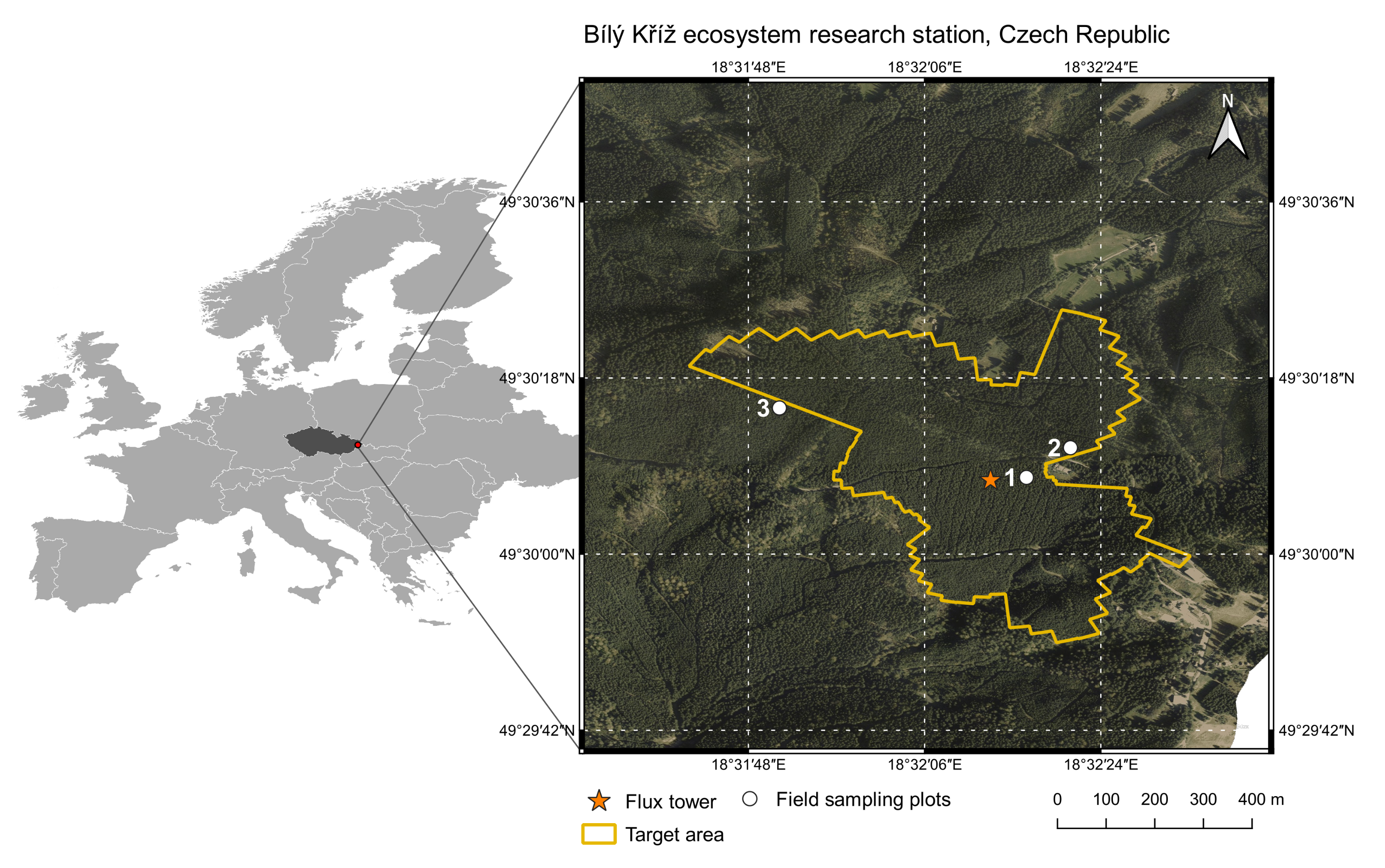
2. Study Area
3. Materials and Methods
3.1. Data
3.1.1. Remote Sensing Data
3.1.2. Ground Measurements
3.2. Retrieval of Vegetation Properties Time Series Using HLS and Airborne Data and the SCOPE Model
3.3. Simulating Gross Primary Production Using SCOPE Model
3.4. Statistical Evaluation of Model Performance
4. Results
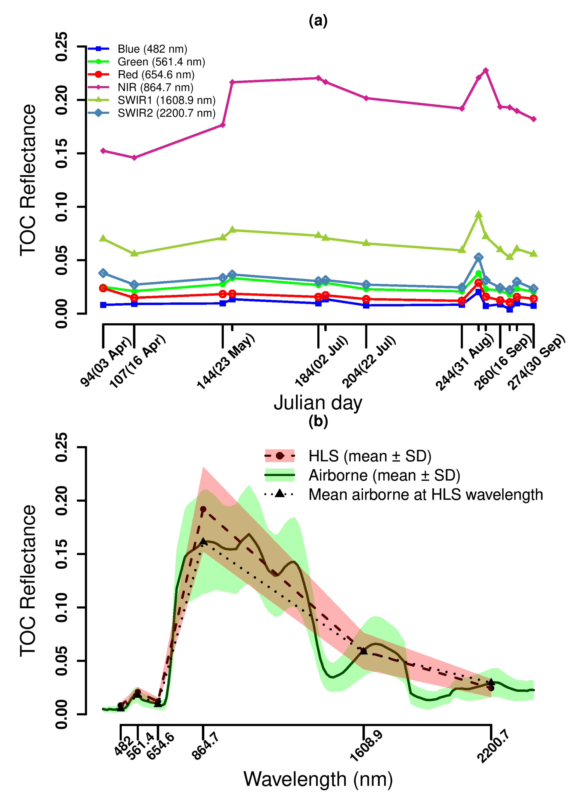
4.1. Variation in Observed Top-Of-Canopy Reflectance
4.2. Simulation of TOC Reflectance
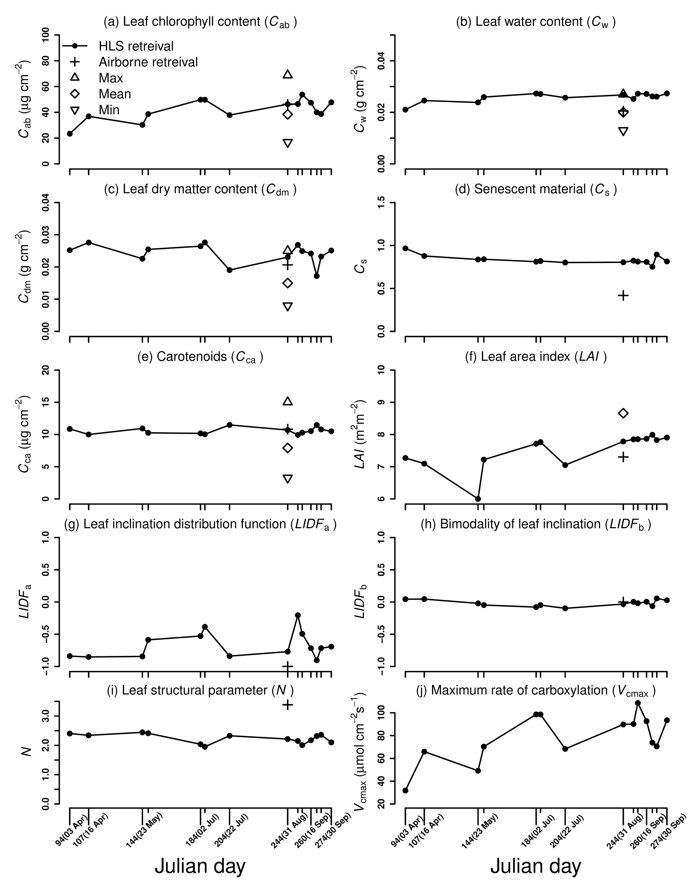
4.3. Retrieval of Vegetation Properties
4.4. Simulations of GPPSIM with SCOPE Model
5. Discussion
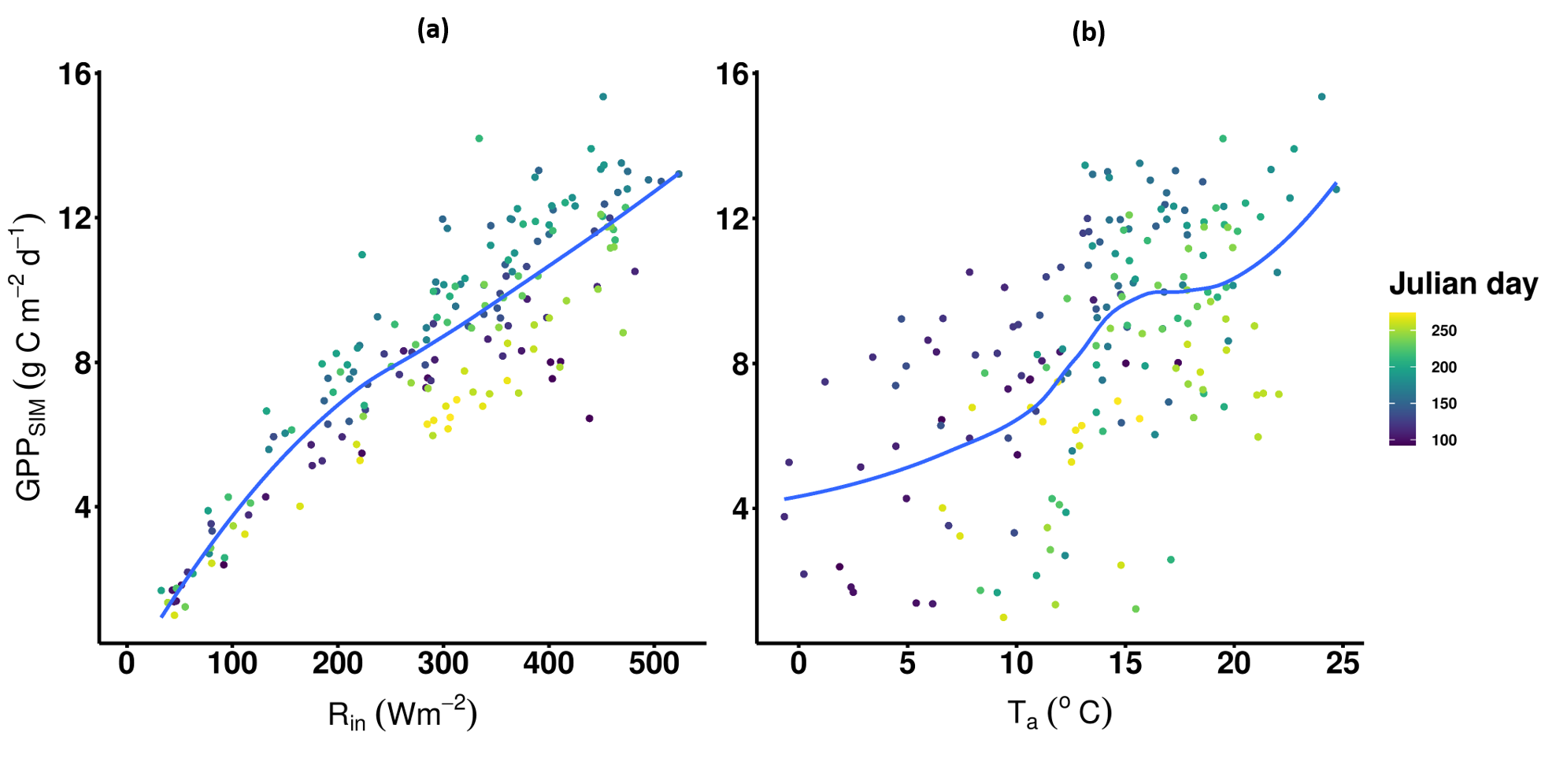
- A temporal increase in is positively correlated with . A previous study, however, did not focus on the temporal aspects of evergreen as well as deciduous tree species, but also found a positive correlation between and [68].
- We observed a good fit between the retrieved vegetation properties and the ground measurements (Section 4.3) on 31 August. At least for one day in the time series, we could therefore validate the retrievals from the HLS TOC reflectance. The retrieved , however, did not exhibit substantial temporal variation. Nevertheless, these variations followed the characteristics of the evergreen tree species, which shows young leaf development phenology during the growing season. These findings agree with those of a previous study on the global spatio-temporal distribution of leaf chlorophyll [69], which highlighted the consistency in the temporal leaf chlorophyll profile of evergreen tree species across the year with an increasing concentration within new needles in spring.
6. Conclusions
- HLS data can provide the dense time series of surface reflectance at the desired locations because it combines data from two existing satellites: Landsat-8 and Sentinel-2. The results demonstrated that the HLS data are capable of preserving the needed information about vegetation properties. We investigated the retrieval only for one evergreen tree species. Nevertheless, our analysis has an important implication for the future use of HLS data for the dense time series retrieval of vegetation properties, which is needed for other tree species, such as deciduous species, showing strong temporal phenology.
- We did not observe any improvement in GPP using the time-varying vegetation properties retrieved from the HLS data. We observed the influence of the time-varying maximum rate of carboxylation () on GPP. However, the empirical relationship used to estimate from leaf chlorophyll content () decreased the accuracy of GPP. Future studies need to redefine this empirical relationship.
Supplementary Materials
Author Contributions
Funding
Conflicts of Interest
References
- Anav, A.; Friedlingstein, P.; Beer, C.; Ciais, P.; Harper, A.; Jones, C.; Murray-Tortarolo, G.; Papale, D.; Parazoo, N.C.; Peylin, P.; et al. Spatiotemporal Patterns of Terrestrial Gross Primary Production: A Review. Rev. Geophys. 2015, 3, 785–818. [Google Scholar] [CrossRef] [Green Version]
- Beer, C.; Reichstein, M.; Tomelleri, E.; Ciais, P.; Jung, M.; Carvalhais, N.; Rödenbeck, C.; Arain, M.A.; Baldocchi, D.; Bonan, G.B.; et al. Terrestrial Gross Carbon Dioxide Uptake: Global Distribution and Covariation with Climate. Science 2010, 329, 834–838. [Google Scholar] [CrossRef] [PubMed] [Green Version]
- Jung, M.; Verstraete, M.; Gobron, N.; Reichstein, M.; Papale, D.; Bondeau, A.; Robustelli, M.; Pinty, B. Diagnostic assessment of European gross primary production. Glob. Chang. Biol. 2008, 14, 2349–2364. [Google Scholar] [CrossRef]
- He, H.; Liu, M.; Xiao, X.; Ren, X.; Zhang, L.; Sun, X.; Yang, Y.; Li, Y.; Zhao, L.; Shi, P.; et al. Large-scale estimation and uncertainty analysis of gross primary production in Tibetan alpine grasslands. J. Geophys. Res. Biogeosci. 2014, 119, 466–486. [Google Scholar] [CrossRef] [Green Version]
- Xiao, J.; Chen, J.; Davis, K.J.; Reichstein, M. Advances in upscaling of eddy covariance measurements of carbon and water fluxes. J. Geophys. Res. Biogeosci. 2012, 117, G00J01. [Google Scholar] [CrossRef] [Green Version]
- Lasslop, G.; Reichstein, M.; Papale, D.; Richardson, A.D.; Arneth, A.; Barr, A.; Stoy, P.; Wohlfahrt, G. Separation of net ecosystem exchange into assimilation and respiration using a light response curve approach: Critical issues and global evaluation. Glob. Chang. Biol. 2010, 16, 187–208. [Google Scholar] [CrossRef] [Green Version]
- Patel, N.R.; Dadhwal, V.K.; Saha, S.K. Measurement and Scaling of Carbon Dioxide (CO2) Exchanges in Wheat Using Flux-Tower and Remote Sensing. J. Indian Soc. Remote. Sens. 2011, 39, 383–391. [Google Scholar] [CrossRef]
- Jung, M.; Reichstein, M.; Margolis, H.A.; Cescatti, A.; Richardson, A.D.; Arain, M.A.; Arneth, A.; Bernhofer, C.; Bonal, D.; Chen, J.; et al. Global patterns of land-atmosphere fluxes of carbon dioxide, latent heat, and sensible heat derived from eddy covariance, satellite, and meteorological observations. J. Geophys. Res. Biogeosci. 2011, 116, G00J07. [Google Scholar] [CrossRef] [Green Version]
- Yu, Q.; Wang, S.; Mickler, R.; Huang, K.; Zhou, L.; Yan, H.; Chen, D.; Han, S. Narrowband Bio-Indicator Monitoring of Temperate Forest Carbon Fluxes in Northeastern China. Remote Sens. 2014, 6, 8986–9013. [Google Scholar] [CrossRef] [Green Version]
- Verma, M.; Friedl, M.A.; Law, B.E.; Bonal, D.; Kiely, G.; Black, T.A.; Wohlfahrt, G.; Moors, E.J.; Montagnani, L.; Marcolla, B.; et al. Improving the performance of remote sensing models for capturing intra- and inter-annual variations in daily GPP: An analysis using global FLUXNET tower data. Agric. For. Meteorol. 2015, 214–215, 416–429. [Google Scholar] [CrossRef] [Green Version]
- Chen, B.; Ge, Q.; Fu, D.; Yu, G.; Sun, X.; Wang, S.; Wang, H. A data-model fusion approach for upscaling gross ecosystem productivity to the landscape scale based on remote sensing and flux footprint modelling. Biogeosciences 2010, 7, 2943–2958. [Google Scholar] [CrossRef] [Green Version]
- Lees, K.J.; Quaife, T.; Artz, R.R.E.; Khomik, M.; Clark, J.M. Potential for using remote sensing to estimate carbon fluxes across northern peatlands—A review. Sci. Total Environ. 2018, 615, 857–874. [Google Scholar] [CrossRef]
- Desai, A.R. Climatic and phenological controls on coherent regional interannual variability of carbon dioxide flux in a heterogeneous landscape. J. Geophys. Res. 2010, 115, G00J02. [Google Scholar] [CrossRef] [Green Version]
- Xiao, J.; Davis, K.J.; Urban, N.M.; Keller, K.; Saliendra, N.Z. Upscaling carbon fluxes from towers to the regional scale: Influence of parameter variability and land cover representation on regional flux estimates. J. Geophys. Res. Biogeosci. 2011, 116, G00J06. [Google Scholar] [CrossRef] [Green Version]
- Ran, Y.; Li, X.; Sun, R.; Kljun, N.; Zhang, L.; Wang, X.; Zhu, G. Spatial representativeness and uncertainty of eddy covariance carbon flux measurements for upscaling net ecosystem productivity to the grid scale. Agric. For. Meteorol. 2016, 230–231, 114–127. [Google Scholar] [CrossRef] [Green Version]
- Raj, R.; van der Tol, C.; Hamm, N.A.S.; Stein, A. Bayesian integration of flux tower data into a process-based simulator for quantifying uncertainty in simulated output. Geosci. Model Dev. 2018, 11, 83–101. [Google Scholar] [CrossRef] [Green Version]
- Constable, J.V.H.; Friend, A.L. Suitability of process based tree growth models for addressing tree response to climate change. Environ. Pollut. 2000, 110, 47–59. [Google Scholar] [CrossRef]
- Running, S.W. Testing Forest-BGC ecosystem process simulations across a climatic gradient in Oregon. Ecol. Appl. 1994, 4, 238–247. [Google Scholar] [CrossRef]
- Van der Tol, C.; Verhoef, W.; Timmermans, J.; Verhoef, A.; Su, Z. An integrated model of soil-canopy spectral radiances, photosynthesis, fluorescence, temperature and energy balance. Biogeosciences 2009, 6, 3109–3129. [Google Scholar] [CrossRef] [Green Version]
- Bayat, B.; van der Tol, C.; Verhoef, W. Integrating satellite optical and thermal infrared observations for improving daily ecosystem functioning estimations during a drought episode. Remote Sens. Environ. 2018, 209, 375–394. [Google Scholar] [CrossRef]
- Verhoef, W.; van der Tol, C.; Middleton, E.M. Hyperspectral radiative transfer modeling to explore the combined retrieval of biophysical parameters and canopy fluorescence from FLEX—Sentinel-3 tandem mission multi-sensor data. Remote Sens. Environ. 2018, 204, 942–963. [Google Scholar] [CrossRef]
- Bayat, B.; van der Tol, C.; Verhoef, W. Retrieval of land surface properties from an annual time series of Landsat TOA radiances during a drought episode using coupled radiative transfer models. Remote Sens. Environ. 2020, 238, 110917. [Google Scholar] [CrossRef]
- Bayat, B.; van der Tol, C.; Verhoef, W. Remote sensing of grass response to drought stress using spectroscopic techniques and canopy reflectance model inversion. Remote Sens. 2016, 8, 557. [Google Scholar] [CrossRef] [Green Version]
- van der Tol, C.; Rossini, M.; Cogliati, S.; Verhoef, W.; Colombo, R.; Rascher, U.; Mohammed, G. A model and measurement comparison of diurnal cycles of sun-induced chlorophyll fluorescence of crops. Remote Sens. Environ. 2016, 186, 663–677. [Google Scholar] [CrossRef]
- Timmermans, J.; Su, Z.; van der Tol, C.; Verhoef, A.; Verhoef, W. Quantifying the uncertainty in estimates of surface–atmosphere fluxes through joint evaluation of the SEBS and SCOPE models. Hydrol. Earth Syst. Sci. 2013, 17, 1561–1573. [Google Scholar] [CrossRef] [Green Version]
- Verrelst, J.; van der Tol, C.; Magnani, F.; Sabater, N.; Rivera, J.P.; Mohammed, G.; Moreno, J. Evaluating the predictive power of sun-induced chlorophyll fluorescence to estimate net photosynthesis of vegetation canopies: A SCOPE modeling study. Remote Sens. Environ. 2016, 176, 139–151. [Google Scholar] [CrossRef]
- Bayat, B.; van der Tol, C.; Yang, P.; Verhoef, W. Extending the SCOPE model to combine optical reflectance and soil moisture observations for remote sensing of ecosystem functioning under water stress conditions. Remote Sens. Environ. 2019, 221, 286–301. [Google Scholar] [CrossRef]
- Vilfan, N.; van der Tol, C.; Yang, P.; Wyber, R.; Malenovský, Z.; Robinson, S.A.; Verhoef, W. Extending Fluspect to simulate xanthophyll driven leaf reflectance dynamics. Remote Sens. Environ. 2018, 211, 345–356. [Google Scholar] [CrossRef]
- Yang, P.; Verhoef, W.; van der Tol, C. The mSCOPE model: A simple adaptation to the SCOPE model to describe reflectance, fluorescence and photosynthesis of vertically heterogeneous canopies. Remote Sens. Environ. 2017, 201, 1–11. [Google Scholar] [CrossRef]
- Claverie, M.; Ju, J.; Masek, J.G.; Dungan, J.L.; Vermote, E.F.; Roger, J.-C.; Skakun, S.V.; Justice, C. The Harmonized Landsat and Sentinel-2 surface reflectance data set. Remote Sens. Environ. 2018, 219, 145–161. [Google Scholar] [CrossRef]
- Lin, S.; Li, J.; Liu, Q.; Li, L.; Zhao, J.; Yu, W. Evaluating the Effectiveness of Using Vegetation Indices Based on Red-Edge Reflectance from Sentinel-2 to Estimate Gross Primary Productivity. Remote Sens. 2019, 11, 1303. [Google Scholar] [CrossRef] [Green Version]
- McGloin, R.; Šigut, L.; Havránková, K.; Dušek, J.; Pavelka, M.; Sedlák, P. Energy balance closure at a variety of ecosystems in Central Europe with contrasting topographies. Agric. For. Meteorol. 2018, 248, 418–431. [Google Scholar] [CrossRef]
- Pastorello, G.; Trotta, C.; Canfora, E.; Chu, H.; Christianson, D.; Cheah, Y.-W.; Poindexter, C.; Chen, J.; Elbashandy, A.; Humphrey, M.; et al. The FLUXNET2015 dataset and the ONEFlux processing pipeline for eddy covariance data. Sci. Data 2020, 7, 225. [Google Scholar] [CrossRef]
- Krupková, L.; Marková, I.; Havránková, K.; Pokorný, R.; Urban, O.; Šigut, L.; Pavelka, M.; Cienciala, E.; Marek, M.V. Comparison of different approaches of radiation use efficiency of biomass formation estimation in Mountain Norway spruce. Trees 2017, 31, 325–337. [Google Scholar] [CrossRef]
- Drápelová, I.; Kulhavý, J. Comparison of soil and seepage water properties in the limed and not-limed spruce forest stands in the Beskydy Mts. Beskydy 2012, 5, 55–64. [Google Scholar] [CrossRef] [Green Version]
- Skakun, S.; Ju, J.; Claverie, M.; Roger, J.-C.; Vermote, E.; Franch, B.; Dungan, J.L.; Masek, J. Harmonized Landsat-8 Sentinel-2 (HLS) Product User’s Guide: Product Version 1.4; National Aeronautics and Space Administration (NASA): Washington, DC, USA, 2018. Available online: Http://hls.gsfc.nasa.gov (accessed on 1 September 2020).
- Hanuš, J.; Fabiánek, T.; Fajmon, L. Potential of airborne imaging spectroscopy at CzechGlobe. Int. Arch. Photogramm. Remote Sens. Spatial Inf. Sci. 2016, XLI-B1, 15–17. [Google Scholar] [CrossRef] [Green Version]
- Homolová, L.; Janoutová, R.; Lukeš, P.; Hanuš, J.; Novotný, J.; Brovkina, O.; Fernandez, R.R.L. In situ data supporting remote sensing estimation of spruce forest parameters at the ecosystem station Bílý Kříž. Beskydy 2017, 10, 75–86. [Google Scholar] [CrossRef] [Green Version]
- Richter, R.; Schläpfer, D. Geo-atmospheric processing of airborne imaging spectrometry data. Part 2: Atmospheric/topographic correction. Int. J. Remote Sens. 2002, 23, 2631–2649. [Google Scholar] [CrossRef]
- Baldocchi, D.D. Assessing the eddy covariance technique for evaluating carbon dioxide exchange rates of ecosystems: Past, present and future. Glob. Chang. Biol. 2003, 9, 479–492. [Google Scholar] [CrossRef] [Green Version]
- Mauder, M.; Cuntz, M.; Drüe, C.; Graf, A.; Rebmann, C.; Schmid, H.P.; Schmidt, M.; Steinbrecher, R. A Strategy for Quality and Uncertainty Assessment of Long-Term Eddy-Covariance Measurements. Agric. For. Meteorol. 2013, 169, 122–135. [Google Scholar] [CrossRef]
- Schotanus, P.; Nieuwstadt, F.T.M.; De Bruin, H.A.R. Temperature measurement with a sonic anemometer and its application to heat and moisture fluxes. Bound. Layer Meteorol. 1983, 26, 81–93. [Google Scholar] [CrossRef]
- Ibrom, A.; Dellwik, E.; Flyvbjerg, H.; Jensen, N.O.; Pilegaard, K. Strong Low-Pass Filtering Effects on Water Vapour Flux Measurements with Closed-Path Eddy Correlation Systems. Agric. For. Meteorol. 2007, 147, 140–156. [Google Scholar] [CrossRef]
- Horst, T.W.; Lenschow, D.H. Attenuation of Scalar Fluxes Measured with Spatially-displaced Sensors. Bound. Layer Meteorol. 2009, 130, 275–300. [Google Scholar] [CrossRef]
- Moncrieff, J.B.; Clement, R.; Finnigan, J.; Meyers, T. Averaging, detrending and filtering of eddy covariance time series. In Handbook of Micrometeorology: A Guide for Surface Flux Measurements; Lee, X., Massman, W.J., Law, B.E., Eds.; Publishing House: Dordrecht, The Netherlands, 2004; pp. 7–31. [Google Scholar]
- Wilczak, J.M.; Oncley, S.P.; Stage, S.A. Sonic Anemometer Tilt Correction Algorithms. Bound. Layer Meteorol. 2001, 99, 127–150. [Google Scholar] [CrossRef]
- Kljun, N.; Calanca, P.; Rotach, M.W.; Schmid, H.P. A Simple Parameterisation for Flux Footprint Predictions. Bound. Layer Meteorol. 2004, 112, 503–523. [Google Scholar] [CrossRef]
- Kormann, R.; Meixner, F.X. An Analytical Footprint Model For Non-Neutral Stratification. Bound. Layer Meteorol. 2001, 99, 207–224. [Google Scholar] [CrossRef]
- Papale, D.; Reichstein, M.; Aubinet, M.; Canfora, E.; Bernhofer, C.; Kutsch, W.; Longdoz, B.; Rambal, S.; Valentini, R.; Vesala, T.; et al. Towards a standardized processing of Net Ecosystem Exchange measured with eddy covariance technique: Algorithms and uncertainty estimation. Biogeosciences 2006, 3, 571–583. [Google Scholar] [CrossRef] [Green Version]
- Reichstein, M.; Falge, E.; Baldocchi, D.; Papale, D.; Aubinet, M.; Berbigier, P.; Bernhofer, C.; Buchmann, N.; Gilmanov, T.; Granier, A.; et al. On the separation of net ecosystem exchange into assimilation and ecosystem respiration: Review and improved algorithm. Glob. Chang. Biol. 2005, 11, 1–16. [Google Scholar] [CrossRef]
- Wutzler, T.; Lucas-Moffat, A.; Migliavacca, M.; Knauer, J.; Sickel, K.; Šigut, L.; Menzer, O.; Reichstein, M. Basic and extensible post-processing of eddy covariance flux data with REddyProc. Biogeosciences 2018, 15, 5015–5030. [Google Scholar] [CrossRef] [Green Version]
- Porra, R.J.; Thompson, W.A.; Kriedemann, P.E. Determination of accurate extinction coefficients and simultaneous equations for assaying chlorophylls a and b extracted with four different solvents: Verification of the concentration of chlorophyll standards by atomic absorption spectroscopy. BBA Bioenerg. 1989, 975, 384–394. [Google Scholar] [CrossRef]
- Jacquemoud, S.; Baret, F. PROSPECT: A model of leaf optical properties spectra. Remote Sens. Environ. 1990, 34, 75–91. [Google Scholar] [CrossRef]
- Verhoef, W.; Bach, H. Coupled soil–leaf-canopy and atmosphere radiative transfer modeling to simulate hyperspectral multi-angular surface reflectance and TOA radiance data. Remote Sens. Environ. 2007, 109, 166–182. [Google Scholar] [CrossRef]
- Rautiainen, M.; Lukeš, P.; Homolová, L.; Hovi, A.; Pisek, J.; Mõttus, M. Spectral Properties of Coniferous Forests: A Review of In Situ and Laboratory Measurements. Remote Sens. 2018, 10, 207. [Google Scholar] [CrossRef] [Green Version]
- Chongya, J.; Hongliang, F. Modeling soil reflectance using a global spectral library. In Proceedings of the AGU Fall Meeting, San Francisco, CA, USA, 3–7 December 2012. [Google Scholar]
- Houborg, R.; Cescatti, A.; Migliavacca, M.; Kustas, W.P. Satellite retrievals of leaf chlorophyll and photosynthetic capacity for improved modeling of GPP. Agric. For. Meteorol. 2013, 177, 10–23. [Google Scholar] [CrossRef]
- Nash, J.E.; Sutcliffe, J.V. River flow forecasting through conceptual models part I: A discussion of principles. J. Hydrol. 1970, 10, 282–290. [Google Scholar] [CrossRef]
- Dumont, B.; Leemans, V.; Mansouri, M.; Bodson, B.; Destain, J.P.; Destain, M.F. Parameter identification of the STICS crop model, using an accelerated formal MCMC approach. Environ. Model. Softw. 2014, 52, 121–135. [Google Scholar] [CrossRef] [Green Version]
- Grabska, E.; Hostert, P.; Pflugmacher, D.; Ostapowicz, K. Forest Stand Species Mapping Using the Sentinel-2 Time Series. Remote Sens. 2019, 11, 1197. [Google Scholar] [CrossRef] [Green Version]
- Chávez, R.O.; Clevers, J.G.P.W.; Herold, M.; Ortiz, M.; Acevedo, E. Modelling the spectral response of the desert tree prosopis tamarugo to water stress. Int. J. Appl. Earth Obs. Geoinf. 2012, 21, 53–65. [Google Scholar] [CrossRef]
- Darvishzadeh, R.; Atzberger, C.; Skidmore, A.; Schlerf, M. Mapping grassland leaf area index with airborne hyperspectral imagery: A comparison study of statistical approaches and inversion of radiative transfer models. ISPRS J. Photogramm. Remote Sens. 2011, 66, 894–906. [Google Scholar] [CrossRef]
- Darvishzadeh, R.; Skidmore, A.; Schlerf, M.; Atzberger, C. Inversion of a radiative transfer model for estimating vegetation LAI and chlorophyll in a heterogeneous grassland. Remote Sens. Environ. 2008, 112, 2592–2604. [Google Scholar] [CrossRef]
- van der Tol, C.; Vilfan, N.; Yang, P.; Bayat, B.; Verhoef, W. Modeling reflectance, fluorescence, and photosynthesis: Developments of the SCOPE model. In Proceedings of the IEEE International Geoscience and Remote Sensing Symposium (IGARSS 2018), Valencia, Spain, 23–27 July 2018. [Google Scholar]
- Verhoef, W.; Bach, H. Simulation of Sentinel-3 images by four-stream surface-atmosphere radiative transfer modeling in the optical and thermal domains. Remote Sens. Environ. 2012, 120, 197–207. [Google Scholar] [CrossRef]
- Verhoef, W.; Bach, H. Simulation of hyperspectral and directional radiance images using coupled biophysical and atmospheric radiative transfer models. Remote Sens. Environ. 2003, 87, 23–41. [Google Scholar] [CrossRef]
- Vilfan, N.; van der Tol, C.; Muller, O.; Rascher, U.; Verhoef, W. Fluspect-B: A model for leaf fluorescence, reflectance and transmittance spectra. Remote Sens. Environ. 2016, 186, 596–615. [Google Scholar] [CrossRef]
- Marenco, R.A.; Antezana-Vera, S.A.; Nascimento, H.C.S. Relationship between specific leaf area, leaf thickness, leaf water content and SPAD-502 readings in six Amazonian tree species. Photosynthetica 2009, 47, 184–190. [Google Scholar] [CrossRef]
- Croft, H.; Chen, J.M.; Wang, R.; Mo, G.; Luo, S.; Luo, X.; He, L.; Gonsamo, A.; Arabian, J.; Zhang, Y.; et al. The global distribution of leaf chlorophyll content. Remote Sens. Environ. 2020, 236, 111479. [Google Scholar] [CrossRef]
- Croft, H.; Chen, J.M.; Zhang, Y.; Simic, A.; Noland, T.L.; Nesbitt, N.; Arabian, J. Evaluating leaf chlorophyll content prediction from multispectral remote sensing data within a physically-based modelling framework. ISPRS J. Photogramm. Remote Sens. 2015, 102, 85–95. [Google Scholar] [CrossRef]
- Darvishzadeh, R.; Skidmore, A.; Abdullah, H.; Cherenet, E.; Ali, A.; Wang, T.; Nieuwenhuis, W.; Heurich, M.; Vrieling, A.; O’Connor, B.; et al. Mapping leaf chlorophyll content from Sentinel-2 and RapidEye data in spruce stands using the invertible forest reflectance model. Int. J. Appl. Earth Obs. Geoinf. 2019, 79, 58–70. [Google Scholar] [CrossRef] [Green Version]
- Luo, X.; Croft, H.; Chen, J.M.; He, L.; Keenan, T.F. Improved estimates of global terrestrial photosynthesis using information on leaf chlorophyll content. Glob. Chang. Biol. 2019, 25, 2499–2514. [Google Scholar] [CrossRef] [Green Version]


| Meteorological Variable | Symbol | Unit | Min | Max | Mean | SD |
|---|---|---|---|---|---|---|
| Air temperature | T | −0.66 | 24.69 | 13.77 | 5.09 | |
| Incoming shortwave radiation | R | 32.57 | 523.19 | 297.87 | 123.21 | |
| Incoming longwave radiation | R | 258.48 | 391.54 | 328.12 | 27.37 | |
| Vapor pressure | e | hPa | 3.44 | 19.49 | 11.50 | 3.41 |
| Air pressure | p | hPa | 895.04 | 925.07 | 914.39 | 5.68 |
| Wind speed | u | 0.77 | 6.90 | 1.85 | 0.97 |
| Parameter | Symbol | Unit | LB | UB | SD | Measured Mean /Range | ||
|---|---|---|---|---|---|---|---|---|
| Biochemical properties | Leaf chlorophyll content | μg cm−2 | 0 | 100 | 50 | 28.8 | 38.42 | |
| Leaf water content | g cm−2 | 0 | 0.05 | 0.025 | 0.01 | 0.02 | ||
| Leaf dry matter content | g cm−2 | 0 | 0.04 | 0.02 | 0.01 | 0.015 | ||
| Senescent material | — | 0 | 1.5 | 0.75 | 0.43 | — | ||
| Carotenoids | μg cm−2 | 0 | 20 | 10 | 5.77 | 7.91 | ||
| Structural properties | Leaf area index | m2 m−2 | 6 | 10 | 8 | 1.15 | 8.66 | |
| Leaf inclination distribution function | — | –1 | +1 | 0 | 0.58 | — | ||
| Bimodality of leaf inclination | — | –1 | +1 | 0 | 0.58 | — | ||
| Leaf structural parameter | N | — | 1 | 3.5 | 2.25 | 0.72 | — | |
| BSM submodel parameters | Soil Brightness parameter | B | — | 0 | 0.9 | 0.45 | 0.26 | — |
| Soil spectral shape latitude | deg | 10 | 50 | 30 | 11.5 | — | ||
| Soil spectral shape longitude | deg | 40 | 70 | 55 | 8.7 | — | ||
| Soil water content | SWC | % | 15.61–31.54 |
| Date of HLS Data | Sensing Satellite | Julian Day | Time of Observation in CET | % of High Quality Pixels | Mean NDVI | Mean SWC (%) at the Time of Observation |
|---|---|---|---|---|---|---|
| 3 April 2016 | S30 | 94 | 11:54:06 | 87.73 | 0.73 | 28.45 |
| 16 April 2016 | L30 | 107 | 11:38:12 | 96.47 | 0.82 | 31.54 |
| 23 May 2016 | S30 | 144 | 11:54:04 | 100 | 0.81 | 23.3 |
| 27 May 2016 | L30 | 148 | 11:32:29 | 100 | 0.84 | 24.94 |
| 2 July 2016 | S30 | 184 | 11:52:19 | 100 | 0.87 | 18.41 |
| 5 July 2016 | L30 | 187 | 11:38:30 | 78.81 | 0.87 | 22.67 |
| 22 July 2016 | S30 | 204 | 11:53:51 | 100 | 0.87 | 25.21 |
| 31 August 2016 | L30 | 244 | 11:33:01 | 100 | 0.88 | 23.37 |
| 7 September 2016 | L30 | 251 | 11:38:50 | 66.91 | 0.81 | 27.23 |
| 10 September 2016 | S30 | 254 | 11:50:27 | 70.45 | 0.87 | 23.52 |
| 16 September 2016 | L30 | 260 | 11:33:04 | 100 | 0.88 | 17.28 |
| 20 September 2016 | S30 | 264 | 11:52:23 | 99.07 | 0.9 | 19.31 |
| 23 September 2016 | L30 | 267 | 11:38:51 | 100 | 0.85 | 18.95 |
| 30 September 2016 | S30 | 274 | 11:50:25 | 51.86 | 0.86 | 15.61 |
Publisher’s Note: MDPI stays neutral with regard to jurisdictional claims in published maps and institutional affiliations. |
© 2020 by the authors. Licensee MDPI, Basel, Switzerland. This article is an open access article distributed under the terms and conditions of the Creative Commons Attribution (CC BY) license (http://creativecommons.org/licenses/by/4.0/).
Share and Cite
Raj, R.; Bayat, B.; Lukeš, P.; Šigut, L.; Homolová, L. Analyzing Daily Estimation of Forest Gross Primary Production Based on Harmonized Landsat-8 and Sentinel-2 Product Using SCOPE Process-Based Model. Remote Sens. 2020, 12, 3773. https://doi.org/10.3390/rs12223773
Raj R, Bayat B, Lukeš P, Šigut L, Homolová L. Analyzing Daily Estimation of Forest Gross Primary Production Based on Harmonized Landsat-8 and Sentinel-2 Product Using SCOPE Process-Based Model. Remote Sensing. 2020; 12(22):3773. https://doi.org/10.3390/rs12223773
Chicago/Turabian StyleRaj, Rahul, Bagher Bayat, Petr Lukeš, Ladislav Šigut, and Lucie Homolová. 2020. "Analyzing Daily Estimation of Forest Gross Primary Production Based on Harmonized Landsat-8 and Sentinel-2 Product Using SCOPE Process-Based Model" Remote Sensing 12, no. 22: 3773. https://doi.org/10.3390/rs12223773