


Abstract
The interaction between interplanetary (IP) shocks and the solar wind has been studied in the past for the understanding of energy dissipation mechanisms within collisionless plasmas. Compared to the study of fast shocks, other types of IP shocks, including slow mode shocks (i.e., fast forward, fast reverse, slow forward, and slow reverse shocks) remained largely unnoticed. We analyze magnetic field fluctuations observed by the Wind spacecraft from 1995 to 2021 upstream and downstream of the IP shocks using a continuous wavelet transform. The evolution of spectral indices in the ion inertial and transition ranges and the changes in distributions of characteristic ion length scales with respect to the spectral break and proton beta are presented. We found that spectral indices in both inertial and transition ranges and the characteristic length scale distributions are statistically conserved across three types of IP shocks, suggesting that mechanisms associated with the energy dissipation are unaffected by the shocks. The results obtained for the transition range of fast reverse shocks show a larger difference between upstream and downstream plasmas and this will be further studied.
Export citation and abstract BibTeX RIS

Original content from this work may be used under the terms of the Creative Commons Attribution 4.0 licence. Any further distribution of this work must maintain attribution to the author(s) and the title of the work, journal citation and DOI.
1. Introduction
Solar wind is a natural laboratory for studying plasma turbulence (Alexandrova et al. 2009; Bruno & Carbone 2013). While a large number of studies of plasma turbulence in the solar wind have been published, relatively less attention has been directed to the interaction between interplanetary (IP) shocks and plasma turbulence. IP shocks are one of the magnetohydrodynamic (MHD) discontinuities formed by nonlinear wave steepening, and can be categorized into different groups; fast forward (FF), fast reverse (FR), slow forward (SF), and slow reverse (SR) shocks (Oliveira 2017). Recently, several studies focus on the nature of plasma turbulence in the upstream and downstream of FF shocks in both theoretical (Zank et al. 2021) and observational (Borovsky 2020) aspects.
When large-scale plasma turbulence (larger than the ion gyroradius in the solar wind) evolves through FF shocks, its power increases and the shape of the downstream power spectral density (PSD) resembles that of upstream (Pitňa et al. 2021a). Similar results are reported by Zhao et al. (2021), indicating that the power of the upstream magnetic field fluctuations is enhanced when they are transmitted to the downstream of FF shocks. However, other shock types have been addressed rarely.
As a method for the study of plasma turbulence, spectral analysis is often adopted. For instance, Pitňa et al. (2016) analyze the spectra of the ion flux fluctuations and Šafránková et al. (2016) calculate the bulk and thermal speed fluctuation spectra in the solar wind. The magnetic field fluctuations are also studied by this method (Alexandrova et al. 2008; Woodham et al. 2018) and the spectra show spectral breaks at or close to typical ion scales (i.e., ion inertial length, λi or ion gyroradius, ρi) that approximately correspond to 0.1–0.3 Hz in the spacecraft frame at 1 au (Alexandrova et al. 2009, 2013, 2021). Many energy dissipating mechanisms such as ion cyclotron resonance, stochastic heating, Landau damping, and magnetic reconnection have been considered for the spectral steepening in the vicinity of the ion scales (Parashar et al. 2015; Bandyopadhyay et al. 2020; He et al. 2020; Alexandrova et al. 2021; Smith & Vasquez 2021). However, the exact physical processes responsible for this spectral break formation are still intensively studied.
On the scale larger than ion inertial length (λi) or ion gyroradius (ρi), the MHD approximation is valid under the assumption that electrons and ions can be treated as a single fluid (Alexandrova et al. 2013; Kiyani et al. 2015). The ion inertial length is defined as λi = VA/Ωp assuming only protons as the solar wind ions, while the ion gyroradius, ρi = Vp,th,⊥/Ωp, where VA = B/ is the Alfvén speed, Vp,th,⊥ is the proton thermal speed perpendicular to the background magnetic field, Ωp = eB/mp is the proton gyrofrequency, μ0 is the permeability of the vacuum, e is the electron charge, B is the magnetic field, Np is the proton number density, and mp is the proton mass. The regime where k
λi ≪ 1 and k
ρi ≪ 1 (k is the wavenumber of the magnetic field fluctuations in the plasma frame) is called the inertial range. The power spectrum of the magnetic field fluctuations in this range evolves with the distance from the Sun from an Iroshnikov–Kraichnan power law with the exponent of −3/2 toward the Kolmogorov-like exponent of −5/3 observed at 1 au (Chen et al. 2020; Zhao et al. 2022b; Šafránková et al. 2023; and references therein).
is the Alfvén speed, Vp,th,⊥ is the proton thermal speed perpendicular to the background magnetic field, Ωp = eB/mp is the proton gyrofrequency, μ0 is the permeability of the vacuum, e is the electron charge, B is the magnetic field, Np is the proton number density, and mp is the proton mass. The regime where k
λi ≪ 1 and k
ρi ≪ 1 (k is the wavenumber of the magnetic field fluctuations in the plasma frame) is called the inertial range. The power spectrum of the magnetic field fluctuations in this range evolves with the distance from the Sun from an Iroshnikov–Kraichnan power law with the exponent of −3/2 toward the Kolmogorov-like exponent of −5/3 observed at 1 au (Chen et al. 2020; Zhao et al. 2022b; Šafránková et al. 2023; and references therein).
Approaching smaller scales that are comparable to or smaller than the ion scales, i.e., k
λi ≥ 1 and k
ρi ≥ 1, the MHD description is no longer valid. This range is often called the ion dissipation range or ion kinetic range and kinetic processes such as the Hall effect become more significant (Alexandrova et al. 2008). Based on Kiyani et al. (2015), this range is called the transition range in our study and the spectral index lies between −2 and −4 (Leamon et al. 1998, 1999; Alexandrova et al. 2009; Sahraoui et al. 2010; Lion et al. 2016). At k
ρi ≥ 1, the transition of Alfvén waves to kinetic Alfvén waves occurs (Schekochihin et al. 2009; Chen et al. 2014) and damping these waves by Landau resonance or other wave–particle interactions leads to the spectrum steepening (Leamon et al. 1999; He et al. 2020). Ion cyclotron resonance is one of the best candidates because it can explain this steepening at the scale of  (defined as
  , where
  and
and  ) by transferring magnetic field energy to resonating protons (Leamon et al. 1998; Chen et al. 2014; Wang et al. 2018; Woodham et al. 2018).
As already noted, the study of the transmission of plasma turbulence across IP shocks is one of the important approaches for understanding its nature (Hu et al. 2012; Pitňa et al. 2021a). With motivation to identify the differences between particular shock types, we extend the scope of the statistical study of the interaction between plasma turbulence and IP shocks in the inertial and transition ranges to four different types of IP shocks, i.e., FF, FR, SF, and SR. We estimate both the up- and downstream spectral properties of the magnetic field fluctuations (the steepness of the spectra and the changes of spectral breaks) and monitor their dependence on proton beta ( /B2).
/B2).
2. Methodology and Data Set
2.1. IP Shock Set
We analyze shocks observed within 1995–2021 by the Wind spacecraft. The identification of IP shocks is based on a detection algorithm suggested by Krupařová et al. (2013). The algorithm uses the jumps of the IP magnetic field (B), the proton number density (Np), and the proton bulk speed (Vp) in the spacecraft frame across the shock front. As briefly introduced in Oliveira (2017), B and Np increase across FF shocks, whereas B decreases and Np increases across SF shock. In reverse shocks, these jumps occur oppositely, but Vp always increases across IP shocks. The profiles of these changes across four types of shocks are shown in Figure 1. Avoiding confusion, we note that the spacecraft observes first upstream of forward (FF and SF) shocks while the order of up- and downstream regions is opposite for reverse (FR and SR) shocks in Figure 1. We compare the identified shocks with two databases: the Database of Heliospheric Shock Waves maintained at University of Helsinki and the CfA IP Shock Database maintained at the Center for Astrophysics. We also add nonduplicating shock events within 1995–2021. In total, 1464 IP shock events were recognized in this stage.
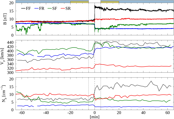
Figure 1. Profiles of solar wind parameters (B, Vp, and Np) as measured across different types of IP shocks: FF (2014 December 21 18:38 UTC, black line), FR (2014 February 17 05:34 UTC, blue line), SF (2013 May 5 17:34 UTC, green line), and SR (2012 December 3 05:31 UTC, red line). Each parameter is shown within [−65 minutes, 65 minutes] from the shock crossing (0 minute, vertical dashed line), and two vertical dotted lines represent ±5 minutes. The blue bars in the top distinguish the intervals of 60 minutes ([−65 minutes, −5 minutes] and [5 minutes, 65 minutes]) where the spectral analysis of the magnetic field fluctuations is applied, while the yellow bars indicate 15 minutes intervals ([−20 minutes, −5 minutes] and [5 minutes, 20 minutes]) for computation of the shock parameters.
Download figure:
Standard image High-resolution imageWe use 1 hr intervals of Wind magnetic field data (blue bars in Figure 1) measured by the Magnetic Field Instrument (MFI) with 92 ms resolution (Lepping et al. 1995) for both upstream and downstream regions skipping 5 minutes prior to and after the shock in order to avoid potential wave effects often occurring in the vicinity of shocks. Data gaps shorter than 92 s (<1000 measurements) are linearly interpolated and shocks with longer gaps are discarded from the data set. We employ Solar Wind Experiment (SWE) data with 98 s resolution for the measurements of Vp, Vp,th,⊥, and Np (Ogilvie et al. 1995). The characteristic proton length scales and β are estimated within the interval of 15 minutes for up- and downstream omitting 5 minutes intervals from the shock vicinity (yellow bars in Figure 1). Events containing less than 5 measurements (≈8 minutes) for either up- or downstream are not considered.
2.2. Magnetic Field Spectra and the Spectral Break Determination
For the estimation of the upstream and downstream PSD of magnetic field fluctuations, we adopt continuous wavelet transform with a Morlet wavelet (ω0 = 6; Torrence & Compo 1998). To determine the break frequency, fb, where the slope of the power spectra abruptly steepens, we fit each spectrum by minimizing χ squared with two-segment piecewise linear function in the log–log space defined as
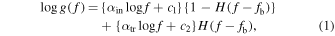
where f is the frequency, c1 and c2 are parameters of the fit, αin corresponds to the inertial range spectral index,  does to the transition range, and H is the Heaviside function. In order to avoid noise effect on the analysis of magnetic field fluctuations, we follow the methodology suggested by Pitňa et al. (2021b), which introduces a noise level estimated by Woodham et al. (2018), and we multiply the noise floor by a factor of 5 (SNR5) as shown in Figures 2(a)–(d) (dashed–dotted green lines). This fitting method is applied in a frequency range from 0.03 to 3 Hz or to the frequency where the PSD level is equal to SNR5 if it is lower than 3 Hz. Using the Taylor hypothesis (Taylor 1938), fb in the spacecraft frame can be converted into the corresponding wavenumber, kb, in the plasma frame moving along the spacecraft with the speed of Vp as kb = 2π
fb/Vp. When the level of the magnetic field fluctuations is comparable to SNR5 at the ion scales or a "bump" is found on the spectrum, the spectral breaks cannot be clearly determined by the fitting method. Thus, only IP shocks containing clear spectral breaks for both up- and downstream spectra are analyzed to an accurate division between the inertial and the transition ranges. The final set of IP shocks contains 306 FF, 113 FR, 109 SF, and 63 SR shocks.
does to the transition range, and H is the Heaviside function. In order to avoid noise effect on the analysis of magnetic field fluctuations, we follow the methodology suggested by Pitňa et al. (2021b), which introduces a noise level estimated by Woodham et al. (2018), and we multiply the noise floor by a factor of 5 (SNR5) as shown in Figures 2(a)–(d) (dashed–dotted green lines). This fitting method is applied in a frequency range from 0.03 to 3 Hz or to the frequency where the PSD level is equal to SNR5 if it is lower than 3 Hz. Using the Taylor hypothesis (Taylor 1938), fb in the spacecraft frame can be converted into the corresponding wavenumber, kb, in the plasma frame moving along the spacecraft with the speed of Vp as kb = 2π
fb/Vp. When the level of the magnetic field fluctuations is comparable to SNR5 at the ion scales or a "bump" is found on the spectrum, the spectral breaks cannot be clearly determined by the fitting method. Thus, only IP shocks containing clear spectral breaks for both up- and downstream spectra are analyzed to an accurate division between the inertial and the transition ranges. The final set of IP shocks contains 306 FF, 113 FR, 109 SF, and 63 SR shocks.
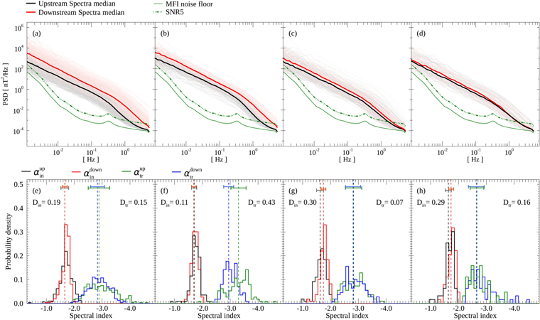
Figure 2. Upper panels: up- (black) and downstream (red) spectra with their median lines for FF (a), FR (b), SF (c), and SR (d) shocks. The MFI noise floor (Woodham et al. 2018) is represented by a green solid line, and SNR5 is a green dashed line. Lower panels: histograms of spectral indices in the upstream and downstream inertial range,  (black), and
  (red), the upstream and downstream transition range
  (green), and
  (blue) for FF (e), FR (f), SF (g), and SR (h). Din and
  in the top denote the maximum difference between the up- and downstream cumulative distributions for the inertial and transition ranges, respectively.
Download figure:
Standard image High-resolution image3. Comparison of Spectral Properties
The PSD of the magnetic field and the histogram of spectral indices in the inertial and transition ranges for four different types of IP shocks are shown in Figure 2. Figures 2(a)–(d) present the individual spectra as well as their medians in up- (black) and downstream (red) of FF, FR, SF, and SR shocks, respectively. A considerable increase of the PSD power from up- to downstream is observed for FF and FR shocks, as reported by many studies (Lu et al. 2009; Pitňa et al. 2021a). The power enhancement by a factor of 5 on average is found across FF shocks (Figure 2(a)), while in FR shocks, the fluctuation power increase approximately by a factor of 3 (Figure 2(b)). The different levels of enhancements for FF and FR shocks can result from the relatively lower Mach number of FR shocks (Pitňa et al. 2021a). On the contrary, a lower power enhancement (≈ by a factor of 1 to 2 on average) is observed for SF (Figure 2(c)) and SR (Figure 2(d)) shocks.
Figures 2(e)–(h) show the histograms of spectral indices for the inertial range upstream (black solid) and downstream (red solid) and for the transition range upstream (green solid) and downstream (blue solid), respectively. Spectral indices in both inertial and transition ranges seem to be statistically conserved across FF, SF, and SR shocks. On the other hand, a steeper upstream spectral index is observed in the transition range for FR shocks (Figure 2(f)), while the inertial range spectral index does not exhibit any significant change. We will return to this point and will quantify the differences in the discussion section.
Figures 3(a), (c), (e), and (g) show the distributions of the ratio between the length scales corresponding to ρi and the spectral break, kρ /kb as a function of β for up- (gray dots) and downstream (red dots) shocks. As it could be expected (Chen et al. 2014), the spectral break tends to be observed at a larger scale than ρi in the low β (β ≪ 1) regime and converges to ρi as β increases (β ≫ 1). There is a small difference between the upstream and downstream distributions that can be seen in the histograms (Figures 3(b), (d), (f), and (h)). The gyroradius scale dependence on β conserves its shape across the shocks, but the points move toward the higher β region in the downstream, especially for SF and SR shocks (Figures 3(e) and (g)).
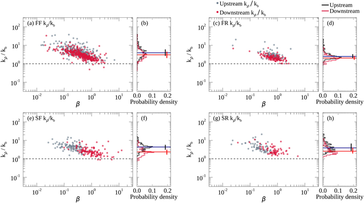
Figure 3. The distributions of the length scale of proton gyroradius (kρ ) normalized to the spectral break scale (kb) as a function of β for the up- (gray dots) and downstream (red dots) of FF (a), FR (c), SF (e), and SR (g) shocks. The up- (black solid line) and downstream (red solid line) histograms of FF (b), FR (d), SF (f), and SR (h) are presented. The black and red horizontal lines in the histograms indicate the median values with the interquartiles.
Download figure:
Standard image High-resolution imageConsidering the change of the plasma parameters, the ratio of βdown/βup > 1 where the superscripts "up" and "down" represent the upstream and downstream parameters, respectively, is always satisfied for SF and SR shocks. However, the convergence of the spectral break toward the proton gyroradius as β increases is still observed. This leads to the shift of distributions to the smaller scale as seen in Figures 3(f) and (h).
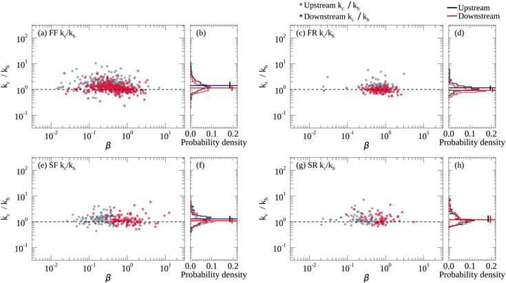
We plotted also the dependence of the kλ /kb ratio as a function of β (not shown) and the trends were complementary. For this reason, Figures 4(a), (c), (e), and (g) show the distributions of the kc/kb ratio between the length scales corresponding to the proton cyclotron resonance and the spectral break as a function of β for the up- (gray dots) and downstream (red dots) shocks. One can see that the upstream and downstream ratios are distributed around unity. Although the increase of β is observed in the downstream SF and SR shocks, the spectral break also tends to occur near the scale of proton cyclotron resonance. Histograms in Figures 4(b), (d), (f), and (h) exhibit little or no correlation of the overall distributions of kc/kb with β. It can be argued that the proton cyclotron resonance is probably responsible for the spectral steepening and that this mechanism is not influenced by IP shocks.
Figure 4. The distributions of the length scale of proton cyclotron resonance (kc) normalized to the spectral break scale (kb) again as a function of β. The format follows Figure 3.
Download figure:
Standard image High-resolution image
4. Discussion and Conclusion
We investigate the change of the spectral slopes of magnetic field fluctuations and the variation of the spectral break scale with respect to proton gyroradius and proton cyclotron resonance scales for four different types of IP shocks. An overview of results is summarized in Table 1. The median and interquartile values of upstream and downstream PSD slopes in both inertial and transition regions (columns (9), (10), (11), (12)), length scale ratios (columns (13), (14)) together with the number of events (column (3)), the percentage of quasi-perpendicular shocks (the angle between the shock normal and the upstream average magnetic field >45°) in a particular shock set (column (4)), the median upstream proton speed averaged within 1 hr interval (column (5)), β (column (6)), and magnetosonic Mach number (column (7)). Fast and slow magnetosonic Mach numbers are considered for fast (FF and FR) and slow (SF and SR) shocks, respectively. The down- to upstream inertial range PSD ratio (column (8)) is estimated for the frequency range of f ≈ [0.003, 0.03 Hz] in the spacecraft frame. In Table 1, we see that FR shocks are observed dominantly in high Vp environments; thus we select a subset of FF shocks with a similar number of events with the upstream proton speed  km s−1 for a direct comparison of FR and FF shocks (see the second row of the table).
Table 1. Number of Events and Median Values with Interquartiles of Parameters
| # Events | # Quasi-⊥ (%) |
 (km s−1) (km s−1) | βup |

|
 / /
|

|

|

|

| (kc/kb)up | (kc/kb)down | ||
|---|---|---|---|---|---|---|---|---|---|---|---|---|---|
| (1) | (2) | (3) | (4) | (5) | (6) | (7) | (8) | (9) | (10) | (11) | (12) | (13) | (14) |
| Fast | Forward | 306 | 76.9 | 373.12 ± 50.55 | 0.37 ± 0.21 | 1.83 ± 0.55 |

| −1.66 ± 0.14 | −1.66 ± 0.08 | −2.89 ± 0.39 | −2.83 ± 0.25 |

|

|
| Forward (sub) | 114 | 69.3 | 466.25 ± 48.59 | 0.40 ± 0.20 | 1.82 ± 0.52 |

| −1.64 ± 0.13 | −1.66 ± 0.07 | −3.15 ± 0.31 | −3.00 ± 0.25 |

|

| |
| Reverse | 113 | 85.0 | 608.05 ± 53.54 | 0.73 ± 0.21 | 1.49 ± 0.27 |

| −1.70 ± 0.09 | −1.70 ± 0.08 | −3.30 ± 0.27 | −2.95 ± 0.18 |

|

| |
| Slow | Forward | 109 | 85.3 | 417.76 ± 51.42 | 0.21 ± 0.11 | 2.30 ± 1.75 |

| −1.63 ± 0.12 | −1.75 ± 0.08 | −2.83 ± 0.29 | −2.81 ± 0.27 |

|

|
| Reverse | 63 | 77.8 | 421.50 ± 64.18 | 0.23 ± 0.10 | 2.74 ± 1.64 |

| −1.63 ± 0.11 | −1.73 ± 0.09 | −2.66 ± 0.25 | −2.64 ± 0.28 |

|

|
Note. A subset from FF shocks ("sub") where  km s−1 is considered in order to compare with FR shocks. The superscripts "up" and "down" are the upstream and the downstream parameters, respectively. The subscript "in" denotes the inertial range from 0.003 to 0.03 Hz in the spacecraft frame. Fast magnetosonic Mach numbers are considered for fast (FF and FR) shocks, while slow magnetosonic Mach numbers are for slow (SF and SR) shocks.
Download table as: ASCIITypeset image
We note that the median parameters of our sets are consistent with the findings of Kilpua et al. (2015), who analyze the properties of FF and FR shocks with respect of their drivers and show that stream interaction region (SIR)- and IP coronal mass ejection (ICME)-driven FF and FR shocks are typically preceded by different types of solar wind. They find that the median upstream solar wind speed is significantly higher for FR shocks than for FF shocks (599 and 383 km s−1, respectively, in their case) and the upstream β values are clearly higher for FR than FF shocks.
It is important to note that the final set of IP shocks consists of 591 shocks with well determined parameters from the initially identified 1464 shocks because we excluded the IP shocks lacking clear up- or downstream spectral break due to a low upstream power comparable to SNR5 or "bumps" on the spectra. The latter condition is characteristic for quasi-parallel shocks where the reflected particles excite low-frequency ion instabilities (Gary 1991; Wilson et al. 2017) and thus, our set contains predominantly quasi-perpendicular or low Mach number quasi-parallel shocks where these effects are not important. Nevertheless, the plots like Figure 2 for subsets of quasi-parallel and quasi-perpendicular shocks (not shown) do not reveal any notable difference.
In comments to Figure 2, we note amplified magnetic field fluctuations in the downstream of fast shocks with an average enhancement factor of approximately 3–5 and this trend is quantified in the column (8) of Table 1. By contrast, slow shocks exhibit smaller or negligible enhancements. As only the transverse component of the magnetic field to the shock normal is amplified (McKenzie & Westphal 1969; Borovsky 2020; Zank et al. 2021), one can speculate that a higher portion of quasi-perpendicular shocks in the set can contribute to the larger PSD enhancement. This trend can be observed in slow shocks because Table 1 shows that 85.3% of quasi-perpendicular SF shocks result in a more significant intensification of fluctuations than 77.8% of SR shocks. However, 85.0% of FR quasi-perpendicular shocks mostly driven by SIRs do not exhibit larger enhancements than 76.9% of FF shocks driven by the ICME or SIR (Kilpua et al. 2015; Pitňa et al. 2021a). Additionally, FF and SF quasi-perpendicular shocks (76.9% and 85.3%, respectively) have remarkably different levels of the power enhancement. The systematic differences in shock drivers likely lead to variations of the compression ratio (and Mach numbers as shown in Table 1), which, in turn, results in the variations in enhancement of magnetic field fluctuations. Thus, a larger power increase across FF than FR shocks is probably driven by its higher magnetosonic Mach number ≈1.83 compared to the FR Mach number ≈1.49. Similarly, as the Mach number of FF shocks is expected to be higher than that of slow shocks, greater power enhancement is observed in FF than SF shocks. However, although SR shock Mach numbers (≈2.74) are higher than those of SF shocks (≈2.30), SF shocks exhibit larger enhancement of the fluctuation power than SR. In order to investigate the increment of fluctuations across IP shocks, a simultaneous consideration of the shock geometry with a Mach number seems necessary.
Bottom panels in Figure 2 present distributions of spectral indices of upstream and downstream spectra. The median values shown in Table 1 agree for all groups of shocks if the statistical errors are taken into account. In order to check whether the upstream and downstream distributions correspond to the same process, we have performed the Kolgomorov–Smirnov (KS) two-sample test. The maximum differences between the up- and downstream cumulative distributions for the inertial (Din) and transition ranges ( ) are given in the top part of lower panels in Figure 2. The comparison of Din and
  with the values D0.001 corresponding to the 0.001 significance level that are given by the number of events in particular set (D0.001 = 0.16, 0.26, 0.26, and 0.35 for FF, FR, SF, and SR shocks, respectively) reveals that Din is slightly larger than D0.001 for FF and SF shock sets but a larger difference between
  and D0.001 (0.43 versus 0.26, respectively) is found for the FR shock set. Since differences between Din and D0.001 for the inertial range are small and determination of the slope suffers with a very large uncertainties connected, for example, with the selection of the frequency range for their determination, we can conclude that we did not find a strong support for the hypothesis that FF, SF, and SR shocks change the turbulence properties in the inertial and transition ranges of frequencies.
A weak flattening of the spectrum across FR shocks that was already mentioned is consistent with the dependence of the transition range slope on the speed. We performed the analysis of slopes as a function of the speed (not shown) and found that steepening of transition range slopes with an increasing velocity is clear visible for all IP shock types. The consistent results are suggested by Zhao et al. (2022a) and by Bruno et al. (2014). Another aspect is that there is a systematic difference between drivers of slow and fast shocks because whereas ICMEs or SIRs are typical drivers of fast shocks, magnetic reconnection is believed to be associated with slow shocks (Zhou et al. 2018; Pitňa et al. 2021a; Wang et al. 2023). On the other hand, it is a question whether slow IP shocks are consistently driven by magnetic reconnection. Gosling (2012), Enžl et al. (2014), and Wang et al. (2023) estimate a typical time interval for observations of reconnection exhausts at 1 au, which would generate downstream of slow IP shocks, to be of the order of 1 minute. However, all slow shocks in our set have significantly longer downstream intervals, suggesting that slow IP shock drivers require further investigations for a reasonable comparison of differences with fast shocks. Nevertheless, Figures 3 and 4 confirm that the most slow shocks are identified in the low proton-beta plasma as suggested by Gosling (2012), i.e., ≈0.21 and 0.23 for SF and SR presented in Table 1, respectively, whereas the observations of fast shocks do not exhibit any β preference.
As presented in Figures 3 and 4, despite the β increase in the downstream of slow IP shocks, the overall trend of the ion length scales depending on β is not influenced by any type of the shock. We are showing it for kρ /kb and kc/kb, and the trend of the inertial length scale relative to spectral break (kλ /kb) that is not shown is also unaffected due to its complementary correlation with kρ /kb following from the kc definition. A similar conclusion follows from the investigation of the PSDs of the solar wind bulk and thermal speeds by Šafránková et al. (2016).
We focus on the statistical analysis of the impact of different IP shocks on the spectral properties of magnetic field fluctuations and energy dissipation mechanisms. Although IP shocks amplify the power of fluctuations in the downstream, our results indicate that the spectral slopes and mechanisms causing the spectral steepening at the ion scales are conserved across three types of IP shocks. Finally, we conclude that our hypothesis that the IP shocks only rescale the characteristics of turbulence without substantial modification of the ion-scale energy dissipation mechanisms cannot be rejected. Our study confirms these statements for FF, SF, and SR shocks; the results for the FR shocks will be a subject of further investigations.
Acknowledgments
The authors acknowledge the use of MFI and SWE data from the Wind spacecraft (https://wind.nasa.gov/data.php). We also acknowledge the use of IP shock database via Center for Astrophysics, Harvard University, USA (https://lweb.cfa.harvard.edu/shocks/wi_data/) and University of Helsinki, Finland (http://www.ipshocks.fi). We thank Gilbert Pi for valuable suggestions. The present work is supported by the Czech Science Foundation under contract 23-06401S and the Charles University Grant Agency under contract 280423. L.Z. and A.S. acknowledge the partial support of NASA awards 80NSSC20K1783 and 80NSSC23K0415.