


Abstract
Statistical studies have found a close association between large solar energetic particle (SEP) events and fast and wide coronal mass ejections (CMEs). However, not all fast and wide CMEs have an associated SEP event. From the Coordinated Data Analysis Web catalog of CMEs observed by the Solar and Heliospheric Observatory (SOHO) between 2009 January 1 and 2014 September 30, we select fast (plane-of-sky speed >1000 km s−1) and wide (plane-of-sky angular width >120°) CMEs and determine whether >20 MeV protons were detected by either SOHO or the Solar TErrestrial RElations Observatory (STEREO-A or STEREO-B). Among the 123 selected CMEs, only 11 did not produce a >20 MeV proton intensity increase at any of the three spacecraft. We use multispacecraft coronagraph observations to reevaluate the speeds and widths of the CMEs. The 11 CMEs without observed >20 MeV protons tend to be in the narrow and slow end of the distribution of the selected CMEs. We consider several factors that might play a role in the nonobservation of high-energy particles in these events, including (1) the ambiguous determination of the CME parameters, (2) the inefficiency of the particle sources to produce >20 MeV protons, (3) the lack of magnetic connection between particle sources and any spacecraft, and (4) the lack of particles accelerated and released during the parent solar eruptions. Whereas the extent of the high Mach number regions formed in front of the CME is limited, the characteristic that seems to distinguish those fast and wide CMEs that lack observed >20 MeV protons is a deficit in the release of particles during the solar eruptions.
Export citation and abstract BibTeX RIS
1. Introduction
Many studies have confirmed that large solar energetic particle (SEP) events tend to be associated with fast and wide coronal mass ejections (CMEs). For example, Chandra et al. (2013) found that most of the major SEP events observed (i.e., SEP events with >10 MeV proton peak intensities above 10 (cm2 s sr)−1) near Earth during solar cycles 23 and 24 were associated with halo or partial halo CMEs originating close to central meridian or on the western hemisphere with average plane-of-sky speeds larger than 1200 km s−1. Cliver & D'Huys (2018) stated that the range of plane-of-sky CME speeds associated with >25 MeV proton events observed near Earth from 1997 to 2016 was 366–3387 km s−1 (with a median speed of 1199 km s−1), whereas the range of widths of CMEs associated with >25 MeV proton events was 59°–360° (with a median of 360°). For a general population of CMEs, they obtained a median speed of 424 km s−1 and median width of 46°. In addition, Kahler & Reames (2003) found that in the period 1998–2000 nearly all fast (plane-of-sky speed >900 km s−1) halo CMEs were associated with >20 MeV proton events near Earth, whereas no CMEs with plane-of-sky speeds >900 km s−1 but widths less than 60° were associated with near-Earth >20 MeV SEP events, suggesting that CME width also is a factor in whether an SEP event is observed.
SEP events observed simultaneously by multiple spacecraft distributed in the inner heliosphere are also associated with large and wide CMEs. For example, Richardson et al. (2014) found that every >25 MeV proton event observed by either the Solar and Heliospheric Observatory (SOHO) or any of the two spacecraft of the Solar TErrestrial RElations Observatory (i.e., STEREO-A and STEREO-B) during 2009–2012 had an associated CME, while the SEP events observed simultaneously by the three spacecraft tended to be associated with fast (>1000 km s−1) CMEs. However, the inverse is not necessarily true, i.e., fast and wide CMEs do not always have an associated SEP event. For example, Marqué et al. (2006) examined a small number of CMEs observed above the western solar limb as seen from Earth with a speed greater than 900 km s−1 that had no radio signature of flare-related particle acceleration and found that none produced conspicuous SEP events at Earth. These authors argued therefore that a CME shock without an associated flare is not sufficient to produce SEPs. Swalwell et al. (2017) found that >1500 km s−1 CMEs without a >40 MeV proton enhancement near Earth tend to be associated with X-ray flares of class <M3. On the other hand, Gopalswamy et al. (2017) suggested that the slow evolution of the CME speed at the origin of the solar eruption is a key factor determining the deficit of high-energy particles in SEP events, in contrast to those CMEs that attain high speeds early during the parent solar eruption and drive fast shocks in the low corona, leading to intense production of high-energy particles. All these studies reveal that the absence of high-energy proton increases after the occurrence of fast and wide CMEs, although rare, is not exceptional.
There are several scenarios that might explain the absence of high-energy particles after the occurrence of a fast and wide CME: (1) the observing spacecraft does not establish magnetic connection with the particle sources, (2) the shock initially driven by the CME does not encounter favorable conditions for the acceleration of particles to high energy either because of a lack of suprathermal seed particles or because the background medium does not allow the CME to drive a strong shock that is an efficient accelerator of energetic particles, (3) there are no flare-accelerated particles to contribute directly to the prompt SEP event and/or provide a seed population for the shock, and (4) accelerated particles are not able to propagate to (or reach) the observing spacecraft. We note that the inefficiency of the shock to accelerate particles might occur across the whole shock front or in localized regions that happen to be magnetically connected to the spacecraft.
In this article we analyze the factors that might have contributed to the nonobservation of >20 MeV protons after the occurrence of fast and wide CMEs. Since an absence of a proton event at a single spacecraft might not be enough to determine whether a fast CME does not produce >20 MeV protons, we use the multiple vantage points that STEREO-A, STEREO-B, and near-Earth spacecraft provided near 1 au during the rising and maximum phase of solar cycle 24. In particular, we analyze whether (1) magnetic connection, (2) the lack of particle release during the parent solar eruptions, or (3) the properties of the shocks presumably driven by the CMEs are factors that may have played a role in the lack of observation of >20 MeV protons. The use of simultaneous observations from three widely separated spacecraft allows us to (1) lower the possibility that no SEP event was detected because no spacecraft was connected to the putative sources of SEPs with respect to those studies performed using single point measurements and (2) use three points of view to determine the 3D large-scale structure of the shocks driven by the CMEs and thus reevaluate the CME parameters. For this reason, we consider fast and wide CMEs during the time interval when the two STEREO spacecraft were still operative and well separated from Earth, i.e., from 2009 January 1, when the spacecraft were ∼45° from Earth, to 2014 September 30, before losing contact with STEREO-B. The distribution of spacecraft during this period allows us to determine whether the lack of high-energy particles was due to poor magnetic connection between spacecraft and the particle sources and analyze the properties of the CMEs as sources of energetic particles. The three spacecraft vantage points allow us to reconstruct the large-scale structure of the CMEs (Kwon et al. 2014) and thus characterize the 3D kinematics of the CMEs and analyze their association with the possible acceleration of high-energy particles (e.g., Lario et al. 2016, 2017a, 2017b; Rouillard et al. 2016; Plotnikov et al. 2017; Kouloumvakos et al. 2019).
In Section 2 we describe the criteria used to select fast and wide CMEs not associated with >20 MeV proton intensity increases as observed by STEREO-A, STEREO-B, and near-Earth spacecraft. In Section 3 we analyze the type III radio bursts observed in association with these CMEs as a signature of particle release (specifically electrons) during the solar eruptions at the origin of the CMEs. Section 4 discusses how well the cataloged CME speeds and widths characterize CMEs that do not display coherent evolutions. In Section 5 we discuss the effects that intervening interplanetary structures have in the nonobservation of >20 MeV protons. In Section 6 we determine the properties of the CMEs that are not associated with observed >20 MeV proton events. In particular, we follow the evolution of the Alfvén Mach number of the front wave formed ahead of the CMEs to determine their capability to accelerate high-energy particles. In Section 7 we discuss the factors that led to the nonobservation of >20 MeV protons during the selected events. Finally, in Section 8 we summarize the results of these analyses and the main conclusions of this work.
2. Selection of Events
From the list of CMEs in the Coordinated Data Analysis Web (CDAW) catalog (cdaw.gsfc.nasa.gov/CME_list/; Yashiro et al. 2004) we selected fast (plane-of-sky speed >1000 km s−1) and wide (plane-of-sky angular width >120°) CMEs observed between 2009 January 1 and 2014 September 30. According to prior statistical studies and prediction schemes (e.g., Gopalswamy et al. 2008; Chandra et al. 2013; Swalwell et al. 2017, and references therein), these selection criteria should guarantee that for most of the selected CMEs there will be an associated SEP event. In the CDAW catalog, CMEs are visually identified from images obtained by the C2 and C3 coronagraphs of the Large Angle and Spectrometric Coronagraph Experiment (LASCO) on board SOHO (Brueckner et al. 1995). The CME speed is based on that of the outermost envelope of the CMEs, which is manually identified as the structure that envelopes the CME. Sequences of images are used to determine the plane-of-sky speed based on the fastest point on the leading edge of this outermost envelope. Here, we use the CME speed obtained by fitting a straight line to the height–time measurements of this leading edge that we designate as Vcdaw.
The plane-of-sky angular width of the CMEs in the CDAW catalog is typically measured in the C2 field of view after the width of the structure becomes stable as the CME propagates outward. The angular width is usually determined in an image subtracted from a previous image in time, and it represents the maximum separation angle of the region where the brightness is above a certain value. In this sense, the angular width could include not only the CME flux rope but also the wave fronts formed in front of fast CMEs (Ontiveros & Vourlidas 2009) that can propagate through coronal streamers (Kwon et al. 2013). We designate the plane-of-sky angular width obtained from the CDAW catalog as ωcdaw. CMEs that appear to surround the occulting disk are assigned a width of 360° and termed "halo CMEs," even though often such CMEs are not symmetric around the occulter. Other CME parameters available from the CDAW catalog are the acceleration (Acdaw) obtained from second-order polynomial fits to the height–time measurements of the CME leading edge (when at least three height–time measurements are obtained), the mass of the CME (Mcdaw) computed following the method described in Vourlidas et al. (2010, 2011), and the kinetic energy of the CME (Kcdaw) obtained from the mass Mcdaw and the linear speed Vcdaw.
A total of 123 CMEs listed in the CDAW catalog from 2009 January 1 to 2014 September 30 fulfilled our selection criteria, i.e.,  km s−1 and ωcdaw > 120°. The mean values of plane-of-sky speeds, angular widths, and accelerations for these 123 CMEs are
  km s−1,
  = 305°, and
  = −23.45 m s−2, whereas the median values are 1205 km s−1, 360°, and −21.90 m s−2, respectively. Mcdaw and Kcdaw were provided just for 117 events of these 123 fast and wide CMEs. The mean values of the logarithms of Mcdaw (in grams) and Kcdaw (in ergs) are
  = 15.91 and
  = 31.84, whereas the median values are 15.94 and 31.83, respectively.
For each one of these CMEs, we checked whether any of the three spacecraft STEREO-A, STEREO-B, or SOHO detected an energetic proton intensity enhancement at energies above 20 MeV. We use proton intensities measured in the energy channel 20–25 MeV of the Energetic and Relativistic Nucleon and Electron experiment (ERNE; Torsti et al. 1995) on board SOHO and the 20.8–23.8 MeV channel of the High-Energy Telescope (HET; von Rosenvinge et al. 2008) of the In situ Measurements of Particles and CME Transients suite of instruments (IMPACT; Luhmann et al. 2008) on board STEREO-A and STEREO-B. We have looked for intensity increases using different time averages (from 1 to 15 minutes) to determine whether a >20 MeV proton intensity increase was observed above a low instrumental background. Shortly after the occurrence of these 123 CMEs, energetic proton intensity increases in these proton energy channels were observed by at least one of these spacecraft in 77% of cases (95/123), and only in 11 cases (∼9%) was there no proton enhancement in any of the three spacecraft. For the remaining 17 CMEs the proton intensities in these energy channels were already elevated owing to prior events, and we cannot discern whether a significant new intensity enhancement was registered by any of the three spacecraft. See Richardson et al. (2014) for a list of the speeds Vcdaw and widths ωcdaw of the CMEs producing >25 MeV proton events as observed by STEREO-A, STEREO-B, and/or SOHO.
Figure 1 shows (a) ωcdaw, (b) Acdaw, (c) Mcdaw, and (d) Kcdaw versus Vcdaw for the selected CMEs. The symbols distinguish whether a >20 MeV proton intensity increase was detected (red crosses), not observed (solid blue circles), or unclear owing to elevated pre-event intensities (open gray circles). Figure 1(a) shows that, with the exception of two halo CMEs, the events for which no >20 MeV proton intensity enhancement was observed (blue symbols) correspond to some of the narrowest and slowest CMEs in our sample and are close to the limits of our selection criteria. Figure 1(b) shows the well-known result that fast CMEs tend to have negative accelerations (e.g., Vršnak et al. 2004), but it also shows that the accelerations of the CMEs without >20 MeV protons are comparatively small. Figures 1(c) and (d) show that the selected CMEs have relatively large masses and kinetic energies compared to overall CME averaged quantities (see Table 1 in Vourlidas et al. 2011). Within the selected CMEs, the CMEs without >20 MeV protons have, on average, smaller masses (Figure 1(c)) and smaller kinetic energies (Figure 1(d)), in agreement with the general trend inferred in statistical studies comparing SEP intensities and dynamic properties of CMEs (see Table 1 in Kahler & Vourlidas 2013).
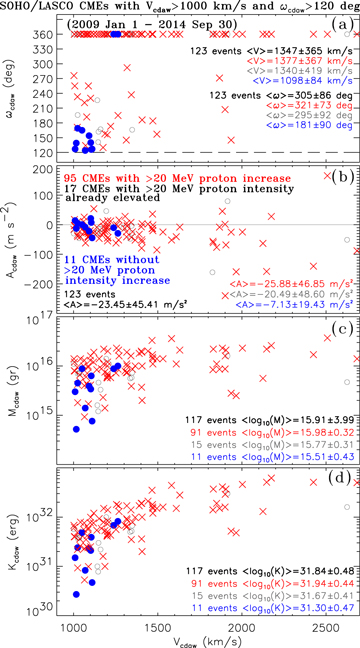
Figure 1. From top to bottom, (a) ωcdaw, (b) Acdaw, (c) Mcdaw and (d) Kcdaw vs. Vcdaw for the selected fast (Vcdaw > 1000 km s−1) and wide ( ) CMEs reported in the CDAW catalog from 2009 January 1 to 2014 September 30. Red crosses indicate CMEs associated with >20 MeV proton intensity increases observed by STEREO-A, STEREO-B, or L1 spacecraft. Blue circles indicate CMEs for which >20 MeV proton intensity increases were not observed by STEREO-A, STEREO-B, or L1 spacecraft. Open gray circles indicate CMEs for which we cannot discern whether a >20 MeV proton intensity increase was observed because the proton intensity was already elevated at the time of the CME. Note that in panels (c) and (d) only 117 events are plotted since masses for six CMEs were not reported in the CDAW catalog.
Download figure:
Standard image High-resolution imageTable 1 provides the main characteristics of these 11 CMEs. We add a "control" CME event (denoted as event ⊕) observed on 2014 February 25 that was accompanied by a >20 MeV proton SEP event. The first three columns of Table 1 list, for each CME, the date and time of the first CME appearance in the LASCO/C2 field of view, the plane-of-sky linear speed (Vcdaw) and angular width (ωcdaw), and the acceleration (Acdaw) and mass (Mcdaw) as reported in the CDAW catalog. The average speed, angular width, acceleration, mass logarithm, and kinetic energy logarithm for these 11 events are  = 1098 km s−1,
  = 181°,
  = −7.13 m s−2,
  = 15.51, and
  = 31.30, whereas the medians are 1092 km s−1, 140°, −8.30 m s−2, 15.59, and 31.36, respectively.
Table 1. Properties of the CME Events without Observed >20 MeV Proton Enhancements
| LASCO CME (CDAW) | Vcdaw/ωcdaw | Acdaw/Mcdaw | Eruption Sitea | Vfit/ωfit (Time) | Vcactus/ωcactus | Type III ∼1 MHz Duration |
|---|---|---|---|---|---|---|
| Date/hh:mm (UT) | (km s−1/deg) | (m s−2/1015 gr) | Long/Lat (time) | (km s−1/deg (UT)) | (km s−1/deg) | (Time, Intensity, Spacecraft) |
| (1) | (2) | (3) | (4) | (5) | (6) | (7) |
| 1 2010 Mar 6/07:51 | 1009/127° | 14.1/3.0 | 250/N24 (07:03) | 1059/074° (07:24–09:39) | 1348e/107° | 4 minutes (07:19–07:23, 1.41 × 10⁵, Wind) |
| 2 2011 Mar 19/12:12 | 1102/140° | 21.3/3.4 | 52-67/S28-S17b (11:33) | 691d/107° (12:39–14:39) | 1201/060° | 0 minutes (0, STA) |
| 3 2011 May 6/08:48 | 1024/169° | 04.8/4.5 | 263/N19 (08:30) | 1065/174° (08:54–10:54) | 1275/142° | <1 minute (08:54–08:54, 1.26 × 10⁴, STB) |
| 4 2011 May 18/18:24 | 1105/>126° | 07.5/6.3 | 320/N10 (18:02) | 1201/161° (18:36–19:54) | 1602/158° | 7 minutes (18:16–18:23, 1.42 × 10⁶, STA) |
| 5 2011 Oct 1/20:48 | 1238/Halo | −10.1/8.8 | 120/N23 (20:26) | 1132/190° (20:40–22:39) | 1294/196° | 15 minutes (20:31–20:46, 5.07 × 10⁶, STB) |
| 6 2011 Dec 19/12:36 | 1092/154° | −22.0/3.9 | 73/S17 (12:00) | 1402/094° (13:30–14:42) | 1329/064° | 5 minutes (12:07–12:12, 2.41 × 10⁴, STA) |
| 7 2012 Jun 23/07:24 | 1263/Halo | −29.1/10.0 | 67-80/N20-N10b (06:50) | 1296/208° (07:54–09:30) | 1953/360° | <1 minute (07:05–07:05, 1.95 × 10⁴, STA) |
| 8 2013 Feb 12/23:12 | 1050/165° | 00.5/8.8 | 167-173/S31-S24b (21:30) | 1049/178° (23:24–00:42) | 1117/118° | 0 minute (0, Wind)f |
| 9 2014 Apr 12/07:24 | 1016/139° | −12.6/5.2 | ∼205/S15 (07:06) | 1015/097° (07:54–09:24) | 1736/060° | 30 minutes (07:10–07:40, 2.33 × 10⁴, STB) |
| 10 2014 May 5/15:24 | 1069/124° | −08.3/1.4 | ∼252/N14 (15:12)c | 1225/091° (15:54–16:54) | 1953/012° | 14 minutes (15:13–15:26, 1.43 × 10⁵, STB) |
| 11 2014 Jul 28/14:30 | 1110/127° | −44.5/7.6 | 259/S10 (13:57)c | 0989/122° (14:39–15:39) | 1491/034° | 18 minutes (13:57–14:15, 1.34 × 10⁵, Wind) |
| ⊕ 2014 Feb 25/01:25 | 2147/Halo | −158.1/22.0 | 103/S12 (00:39) | 2170/250° (00:45–01:54) | ⋯ | 23 minutes (00:48–01:11, 8.13 × 10⁶, STB) |
Notes.
aCarrington coordinates of the parent solar eruption. Units are degrees, and times are given in UT of the day indicated in Column (1). bEruption of a large extended filament at the onset of the events on 2011 March 19, 2012 June 23, and 2013 February 12. cEruption onset time identified by the occurrence of metric type III since EUV images did not allow a precise onset measurement. dSpeed and width determined using the structure identified by the red line in Figure 9. eCACTus incorrectly identified the CME on 2010 March 6 as two separate structures. The listed speed corresponds to the fastest portion of the CME as identified by CACTus, and the width envelopes the two structures. fType III observed mainly at frequencies below 1 MHz and delayed with respect to the parent solar eruption.Download table as: ASCIITypeset image
Figure 2 and 3 show, for each one of these 11 CMEs (together with the control event ⊕ in the bottom right panel of Figure 3), particle intensities measured at STEREO-B (STB), near Earth (L1), and at STEREO-A (STA). In particular, we show 15-minute averages of the proton intensities measured in the 20.8–23.8 MeV proton channel of IMPACT/HET on board STEREO and in the 20–25 MeV proton channel of ERNE on board SOHO (red traces), together with the proton intensities in the 4–6 MeV energy channel of the Low-Energy Telescope on board STEREO (Mewaldt et al. 2008) and the 4–5 MeV channel of SOHO/ERNE (black traces). When a near-relativistic electron intensity enhancement that was clearly associated with the CME of interest (rather than with some other unrelated event) was observed by either the Solar Electron and Proton Telescope (SEPT; Müller-Mellin et al. 2008) on board STEREO or the Deflected Electron (DE) system of the Electron Proton Alpha Monitor (EPAM; Gold et al. 1998) on board the Advanced Composition Explorer (ACE), we plot the ∼40 keV electron intensities observed by these instruments (green traces) unless there is an indication that the SEPT electron channels might be contaminated by protons (e.g., Wraase et al. 2018). Note that the ACE/EPAM/DE channels have a higher instrumental background than those of STEREO/SEPT (see Figure 1 in Lario et al. 2013); therefore, some electron increases at L1 might have been obscured by the high background. Therefore, the green lines in Figures 2 and 3 are only shown when we are confident that a near-relativistic electron increase free of contamination was observed by the spacecraft indicated in the respective panel.

Figure 2. Each panel shows the energetic particle intensities observed at, from top to bottom, STB, L1, and STA for the first six selected CMEs (1 through 6). Red and black traces are for protons, and green traces are for near-relativistic electrons. The purple arrows indicate the CME times. Note that for event 6, L1 observations come from the Electron Proton and Helium Instrument on SOHO (Müller-Mellin et al. 1995) instead of SOHO/ERNE. Various features at individual spacecraft, including stream interaction regions (SIRs), interplanetary coronal mass ejections (ICMEs), and shocks, are also noted.
Download figure:
Standard image High-resolution image
Figure 3. Same as Figure 2, but for the second group of selected CMEs (7 through 11) plus the event ⊕ on 2014 February 25.
Download figure:
Standard image High-resolution imageThe criterion used to select the 11 events is that there is no significant increase in the red traces shown in Figures 2 and 3 at any of the three spacecraft shortly after the occurrence of these 11 CMEs (indicated by the purple arrows; ignore the control event ⊕ in the bottom right panel of Figure 3 when >20 MeV protons were observed and therefore it is not one of the 11 selected events). Note that the stack of detectors of IMPACT/HET allows for measurements clean of instrumental background and hence the discrete red circles in the STA and STB panels that correspond to single counts and contrast with the solid red line in the L1 panel dominated by the SOHO/ERNE instrumental background. We also note that for these 11 CMEs the energetic particle sensor on board the Geostationary Operational Environmental Satellites (GOES) located near Earth did not detect any proton intensity increase at energies >10 MeV. It is also evident that in a few cases in Figures 2 and 3 there is a modest enhancement of 4–5 MeV protons that might be associated with the CME, with another particle source, or with interplanetary processes such as the presence of stream interaction regions (SIRs). For a comparison with these 11 events, the last panel of Figure 3 shows the ∼20 MeV proton intensities observed, from top to bottom, by STEREO-B, SOHO, and STEREO-A during an intense SEP event on 2014 February 25 that was studied in detail by Lario et al. (2016). As already noted, we identify this "control" event with the symbol ⊕ to distinguish it from the other events numbered chronologically from 1 to 11. The last row of Table 1 provides the properties of the CME associated with the origin of this event.
By using extreme-ultraviolet (EUV) observations from the Sun Earth Connection Coronal and Heliospheric Investigation (SECCHI; Wuelser et al. 2004) on board STEREO and/or the Atmospheric Imaging Assembly on board the Solar Dynamics Observatory (SDO/AIA; Lemen et al. 2012), we have identified the site of the parent solar eruption generating each CME. The location of this parent eruption in Carrington coordinates (longitude/latitude) is listed in Column (4) of Table 1. Note that the CMEs 2, 7, and 8 were generated by large filament eruptions that extended over at least ∼15° in longitude or latitude as indicated in Table 1. In Column (4) of Table 1 we also indicate in parentheses the initiation time of the eruptive signatures such as the rise of a filament in events 2, 7, and 8 or the start of the occurrence of an EUV brightening (the resolution of these times is limited by the cadence of the EUV images usually to ±5 minutes in the case of STEREO observations). Note that for events 10 and 11 we use as onset of the eruption the time of metric type III radio emission (see Section 3).
Figure 4 shows, for each one of the 11 selected CMEs plus the control event ⊕, the longitudinal distribution of the spacecraft, as seen from the north ecliptic pole, where the red, blue, and black circles indicate the locations of STEREO-A (STA), STEREO-B (STB), and Earth, respectively, all of them at heliocentric radial distances close to 1 au. The Carrington longitude of each spacecraft (ϕ) is indicated in the figure, together with the longitude of the parent eruption site (purple straight line). The longitude of the parent region as seen from Earth is indicated in purple, whereas the longitude as seen from STEREO-A and STEREO-B is indicated near the STA and STB symbols, in red and blue font, respectively. When the event occurs on (or near) the visible part of the Sun as seen from Earth and a soft X-ray (SXR) flare has been detected, we indicate in parentheses the GOES X-ray class of the flare (using the purple font). All these SXR flares were below class C5. Nominal Parker spiral magnetic field lines connecting each spacecraft with the Sun are also plotted in Figure 4 using the solar wind speed measured by each spacecraft at the time of the CME. We also indicate next to the STA, STB, and Earth symbols the estimate of the longitudinal distance Δψ between the site of the parent solar eruption and the footpoint of the nominal Parker spiral magnetic field line connecting to STEREO-A, STEREO-B, and Earth, respectively. We note that these nominal field lines might differ from the actual topology of the interplanetary magnetic field (IMF) lines at the time of the CME owing to the presence of intervening structures such as interplanetary CMEs (ICMEs), corotating interaction regions (CIRs), and solar wind SIRs. For example, STB in event 7 and Earth in event 4 were immersed in rarefaction regions observed after the crossing of high-speed solar wind streams, where magnetic field tends to be more radial than in a nominal Parker spiral configuration (e.g., Lario & Roelof 2010, and references therein). Figure 4 clearly shows that, in general, the use of three spacecraft assures good coverage in terms of field-line connections to the putative sources of SEPs (assumed to be in the vicinity of or centered approximately on the flare location). In terms of Δψ, the poorest magnetic connection between the site of the parent solar eruption and any of the spacecraft occurred in event 3 (when Δψ for STEREO-A was ∼73°) and event 5 (when Δψ for STEREO-B was ∼83°), whereas for the rest of the events the minimum Δψ among the three spacecraft was always below 40°. The development of a fast and, in principle, wide CME assures us that the connection with a potential CME-driven shock might be established by at least one spacecraft. Therefore, the absence of >20 MeV protons associated with these CMEs at all three spacecraft was not always consistent with the lack of magnetic connection between spacecraft and the SEP sources.

Figure 4. View from the north ecliptic pole showing the location of STEREO-A (STA; red symbol), near-Earth observers (Earth; black symbol), and STEREO-B (STB; blue symbol), at the time of the CME occurrence for each one of the selected events. ϕ indicates the Carrington longitude of each spacecraft. Also shown are nominal IMF lines connecting each spacecraft with the Sun (yellow circle at the center, not to scale) considering the solar wind measured at the time of the CME. The purple line indicates the longitude of the site of the parent solar eruption. The east (E) or west (W) longitude near the STA and STB symbols and near the purple line indicates the longitude of the parent active region as seen from STEREO-A, STEREO-B, and Earth, respectively. Δψ near the STA, STB, and Earth symbols indicates the longitudinal distance between the site of the parent solar eruption and the footpoint of the nominal Parker spiral field line connecting to STEREO-A, STEREO-B, and Earth, respectively.
Download figure:
Standard image High-resolution imageFigure 1 shows that although the 11 CMEs without SEP events are among the narrowest, slowest, and least massive of our selected events, the fact that other CMEs with similar speeds, widths, and masses were able to generate SEPs suggests that the absence of >20 MeV protons in these events should be due to additional reasons rather than the CME parameters per se. Since both ωcdaw and Vcdaw are plane-of-sky measurements retrieved from the CDAW LASCO CME catalog and therefore based on single-point observations, we decided to use the three vantage points provided by STEREO-A, STEREO-B, and SOHO to estimate in 3D the widths and speeds of the CMEs, in particular to see whether the fast and wide classification based on the CDAW catalog is confirmed. We have applied a compound geometrical model developed by Kwon et al. (2014) to represent the 3D geometry of the outermost front of the CME as seen in white-light (WL) images from the SOHO/LASCO and STEREO/SECCHI (Howard et al. 2008) coronagraphs. An ellipsoid shape centered at a certain altitude is used to describe the outermost front of the CME. By using two images when the leading-edge heights were around ∼5 and ∼14 R⊙, we estimated the speed of the ellipsoid leading edge. Column (5) of Table 1 gives the speed of the leading edge of the ellipsoid (Vfit) and angular width of the ellipsoid (ωfit) obtained by using the two times listed in parentheses. Clearly the angular widths obtained when fitting an ellipsoid ωfit are narrower than those listed in the CDAW catalog ωcdaw. The speeds obtained from the ellipsoid fit are comparable to Vcdaw, although in a few cases the speed obtained using the ellipsoid fit Vfit is slower than that listed in the CDAW catalog Vcdaw, and these CMEs would not have fulfilled our speed selection criterion. Other CME catalogs provide different speed and width estimations. For example, Column (6) of Table 1 lists the plane-of-sky width and speed of the leading edge of the selected CMEs as provided by the Computer Aided CME Tracking (CACTus) catalog based on SOHO/LASCO observations (available at sidc.oma.be/cactus/; Robbrecht et al. 2009). Whereas the CME speeds automatically computed by the CACTus algorithms are slightly faster than, but comparable to, Vcdaw, the widths from CACTus are considerably narrower than ωcdaw. Therefore, the selected CMEs would have fulfilled the speed selection criterion when using the CACTus catalog but not the angular width criterion. Prior studies comparing CME parameters from different catalogs pointed out the trend for broader widths in the CDAW catalog with respect to other catalogs (e.g., Richardson et al. 2015; Lamy et al. 2019), which may result from the fact that CME parameters in the CDAW catalog are determined manually by eye, including fainter fronts that other automatic detection algorithms do not consider and using a generous halo CME definition that includes many asymmetric CMEs directed far from the Sun–Earth line. However, because of the widespread use of CME parameters from the CDAW catalog in SEP studies through the last two solar cycles, we have based our selection of fast and wide CMEs on this catalog. In the following sections we analyze possible factors that may have led to the nonobservation of >20 MeV protons associated with these fast and wide CMEs.
3. Type III Radio Emissions
We first consider whether there is any other evidence that particle acceleration occurred in association with these CMEs. In particular, we use type III radio observations to assess whether electrons were accelerated and released during these solar eruptions. SEP events are usually associated with type III (fast drift) radio emissions generally attributed to the escape of flare-accelerated electrons. In particular, large SEP events are nearly always associated with bright, long-lasting type III emissions (e.g., Cane et al. 2002; MacDowall et al. 2003, 2009; Winter & Ledbetter 2015; Richardson et al. 2018). Figures 5 and 6 show the dynamic spectra of the decametric–hectometric (DH) radio emission as observed by the spacecraft that is closest in longitude to the site of the parent solar eruption. The selection of this spacecraft eliminates as much as possible occultation at high frequencies when eruptions occur on the back side of the Sun relative to the observing spacecraft. Data shown come from the WAVES detector (Bougeret et al. 2008) on STEREO and the WAVES experiment (Bougeret et al. 1995) on the Wind spacecraft near Earth. Color bars indicate the flux density of the radio emissions in solar flux units (1 sfu = 10−22 Wm−2 Hz−1), where the data from the different spacecraft have been calibrated using the procedure described in Krupar et al. (2014). We overplot the ∼1.0 MHz time-intensity profile (black or gray traces where the intensity is above or below 5 × 10³ sfu; see discussion below) since the duration of the event near ∼1 MHz is often used to characterize the relationship between type III bursts and SEP production (e.g., MacDowall et al. 2003, 2009). In particular, we show 1.040 MHz flux density in the case of Wind/WAVES measurements and 1.025 MHz in the case of STEREO/WAVES (in sfu units as indicated in the right vertical axis) for the 11 selected events plus the control event on 2014 February 25.
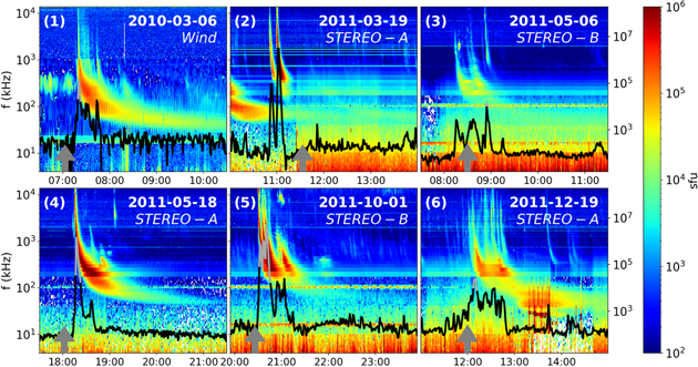
Figure 5. Six dynamic spectra of DH radio emission as observed by the spacecraft closest in longitude to the solar site of the parent solar eruption for the first group of selected events. The 1.040 MHz intensity-time profile (in the case of Wind/WAVES) and 1.025 MHz (in the case of STEREO/WAVES) is overplotted in each panel in sfu units as indicated in the right vertical axis (using black or gray traces when the intensity is above or below 5 × 10³ sfu, respectively as per the criterion described in the text). The gray arrows indicate the onset of the parent solar eruption.
Download figure:
Standard image High-resolution imageThe control event on 2014 February 25 (panel (⊕) in Figure 6) shows the bright, long-lasting type III emissions typical of those accompanying large SEP events (e.g., Cane et al. 2002) that indicate the acceleration and release of electrons during this eruption. There are also also fainter, slower-drifting type II emissions trailing the type III emissions, usually attributed to particle acceleration at a shock, accompanying this CME (cdaw.gsfc.nasa.gov/CME_list/radio/waves_type2.html), as is also typical for large SEP events. In contrast, the other 11 events show weaker emissions, in particular at high (>2 MHz) frequencies, where the type III bursts are of very short duration or are not sufficiently intense to be detectable, although the presence of related emissions at lower frequencies in some of these 11 events suggests that electrons were released. Similarly, the only DH type II (slow drift) radio burst observed in these 11 events occurred in event 5 (see solar-radio.gsfc.nasa.gov/wind/bursts_2011.html), which curiously, among the 11 events, showed the most intense type III emission at high frequencies associated with a group of type III bursts. Thus, the DH radio observations in these 11 events are consistent with weaker particle releases compared to those associated with major SEP events, and apparently they were often limited to a brief period during the eruption.
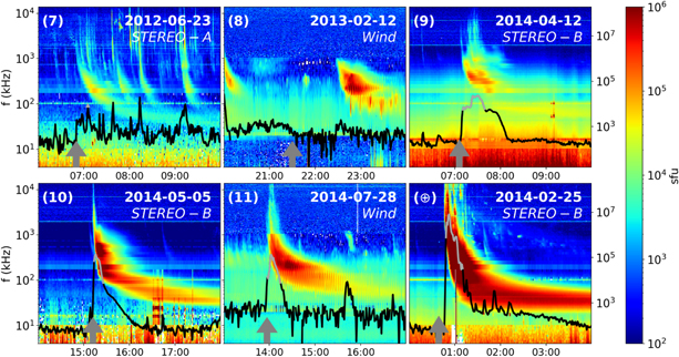
Figure 6. Same as Figure 5, but for the second group of selected events.
Download figure:
Standard image High-resolution imageWe have also checked for ground-based observations of metric type III radio bursts, which are thought to be generated by nonthermal electrons at heights between roughly 0.1 and 1 R⊙ above the photosphere as an indicator of particle acceleration and release in the low corona. The only evidence of metric radio bursts occurring after the time indicated as the origin of the parent eruption in Column (4) of Table 1 obtained from Nançay Decametric Array (NDA) observations at frequencies <100 MHz occurred in events 10 and 11 as counterparts of the DH type III bursts shown in panels (10) and (11) of Figure 6 (in event 10 at ∼15:12 UT on 2014 May 5 and event 11 at ∼13:57 UT on 2014 July 28). For event 6 a noisy storm emission after ∼12:10 UT was observed by NDA (K.-L. Klein 2018, private communication). This event also shows a series of brief type III bursts at DH wavelengths (Figure 5). In addition, Solar Geophysical Data (ftp://ftp.swpc.noaa.gov/pub/indices/events/) report the observation of weak metric type III bursts in event 5 at 20:29 UT by the Palahua Observatory and in event 7 at 07:37 UT by the San Vito Observatory. No other metric radio emissions were observed in association with the rest of events. Therefore, the metric type III radio emissions for the 11 CMEs were weak or not present.
Considering the events with evidence of metric type III ground-based observations (i.e., events 5, 6, 7, 10, and 11), Figures 2 and 3 show that near-relativistic (>40 keV) electron increases were observed at the best nominally connected spacecraft in each case with the exception of event 6. Note that in event 5 the near-relativistic electron intensities at STEREO-B were not observed to increase above an elevated pre-event intensity until ∼4.5 hr after the solar eruption. Near-relativistic electrons were also observed by STEREO-B during event 1 (panel (1) in Figure 2), but no metric type III burst was observed in this case.
MacDowall et al. (2009) found that the average type III burst duration at ∼1 MHz tends to increase with the 25 MeV proton intensity of the associated SEP event (see their Figure 3). For a group of control events where no near-Earth 25 MeV proton intensity increases were detectable, the type III burst duration was always ≲20 minutes, with a mean duration of 12 minutes. We have determined the duration of the type III burst shown in Figures 5 and 6 at the frequencies of 1.040 MHz for Wind and 1.025 MHz for STEREO observations. Such durations are indicated by the gray portion of the overplotted ∼1 MHz intensity profiles in Figures 5 and 6 and have been selected as those time intervals occurring within 25 minutes after the parent solar eruption with ∼1 MHz flux densities above 5 × 10³ sfu (corresponding to the >6 dB criteria previously used by MacDowall et al. 2009). These durations, the time interval defining such durations, and the peak intensity of the observed radio emission are listed in Column (7) of Table 1. Since the type III emission in event 8 occurred mostly at low frequencies and more than 1 hr after the parent solar eruption (Figure 6), we have assigned a null duration to this event. Similarly, we have also assigned a duration of zero minutes for event 2 because the last type III burst shown in panel (2) of Figure 5 occurred before the filament that generated the CME in this event started to rise and hence was unlikely to be associated with the CME. The only emissions possibly associated with this eruption are faint and observed around 100 kHz from ∼12 to 13 UT. In the case of bursty type III emissions such as in events 6 and 7, the duration of the most prominent peak above 5 × 10³ sfu and within the 25 minutes after the onset of the parent eruption has been listed in Column (7) of Table 1.
It is worth pointing out that events 2, 7, and 8 were generated by the disappearance of large solar filaments (DSFs). Event 2 was initiated by a limb prominence observed by SDO/AIA 304 Å that started to rise at ∼11:33 UT on 2011 March 19, with a fast eruption starting at ∼12:06 UT. Event 7 was initiated by a limb prominence observed by SDO/AIA 304 Å that started to rise on 2011 June 23 at ∼06:50 UT and erupted at ∼07:00 UT. In event 8, the filament started to rise very slowly at ∼21:30 UT on 2013 February 12 with a fast eruption starting at ∼22:25 UT. Long-lasting post-eruption two-ribbon arcades were observed in EUV 195 Å images after these DSFs. In particular, the post-eruption arcades appeared to start brightening, with a ±5-minute resolution, at ∼12:30 UT on 2011 March 19 in event 2, at ∼07:05 UT on 2011 June 23 in event 7 (intensifying at 08:00 UT), and at ∼22:30 UT on 2013 February 12 in event 8, and lasted for several hours. Type III radio emissions intensified at these times but at low frequencies (≪1 MHz). Additionally, a GOES C2.7 SXR flare associated with event 7 started at 07:02 UT (maximizing at 07:50 UT), which might be related to the post-eruption arcade brightening.
Column (7) of Table 1 shows that, with the exception of event 9, the burst durations of the events without observed >20 MeV protons are shorter than 20 minutes. For 7 out of the 11 events the ∼1 MHz burst durations are shorter than the 12-minute average found by MacDowall et al. (2009) in their type III bursts without 25 MeV proton increases. The longer durations occurred in events 5, 10, and 11 (all of them with metric type III counterparts but of very short duration) and for event 9, in which a broad low-frequency (≤1 MHz) emission was observed. Therefore, collectively, the burst durations of our selected events are consistent with those without associated SEP events. The weak type III emissions accompanying these CMEs are an indication that they were probably not associated with SEP events, or, at the most, with small particle events.
Additionally, for those events occurring on the visible side of the Sun as seen from Earth and when RHESSI allowed for observations (i.e., events 4, 7, 9, and 10), we have confirmed that no hard X-ray emissions were observed above 25 keV (G. Share 2018, private communication), indicating that no bremsstrahlung emission was generated by electrons accelerated during these solar eruptions. This is further evidence that these eruptions were not efficient accelerators of energetic particles.
4. Ambiguity in the Values of the CME Widths
Recently, Kahler et al. (2019) suggested that fast (>900 km s−1) and narrow (<60°) CMEs move as projectiles through the corona and thus are able to generate just confined bow shocks. By contrast, fast and wide CMEs are able to generate broad shocks formed ahead of a piston driver expanding outward through the corona, accumulating material to produce wide-ranging shocks. According to these authors, the production of high-energy SEPs is favored in the case of broad expansion shocks, whereas projectile-driven shocks produce only low-energy (<10 MeV) particles with narrow injection regions. Therefore, it is important to consider the angular width of the CMEs as a factor discriminating between the production and absence of high-energy SEPs.
The angular width listed in the CDAW catalog ωcdaw is measured in the C2 field of view (∼2.3–6 R⊙) when the width of the structure becomes stable as it propagates outward. However, the CME shape and hence its width may evolve differently below this height (≲2.3 R⊙; e.g., St. Cyr et al. 1999). When estimating the plane-of-sky angular extent of the CMEs, the value of ωcdaw usually encompasses the whole structure, including irregular features that may lead to misrepresentation of the actual CME width. This appears to be the case in events 2, 10, and 11.
Figure 7 shows a sequence of images for event 10 as seen from the SECCHI coronagraphs (COR-1 and COR-2) on board STEREO-B. The CME initially had a narrow jet-like structure as per the definition used in Vourlidas et al. (2017; see Figure 1(c) in that paper). This structure is indicated with a white arrow in the left panel of Figure 7. More than 1 hr later, the initial jet-like structure developed into a more usual, wider CME (right panel of Figure 7). From the point of view of STEREO-B, the angular width never exceeded 100°, whereas the CDAW catalog gives ωcdaw = 124°. In the right panel, there is a brighter, faster feature on the CME front that is aligned with the initial jet-like structure. In fact, the automatic CME identification algorithms of the Solar Eruptive Event Detection System (SEEDS) based on LASCO/C2 data (spaceweather.gmu.edu/seeds/lasco.php) identify only a narrow CME associated with this brighter feature with a width of only 18° moving at a speed averaged over all its angular width of 845 km s−1. Similarly, the CACTus catalog (sidc.oma.be/cactus/catalog/LASCO/2_5_0/2014/05/CME0033/CME.html) also identifies just this narrow feature and gives for this CME a width of only 12° with leading edge moving at 1953 km s−1 and speed decreasing to below <500 km s−1 in less than 10° in position angle. Therefore, this CME would have not met our selection criterion if we used CME parameters from these catalogs. It is also possible that if this CME did drive a shock, it might have been narrow and just along the initial jet direction. This CME was also included in the Space Weather Database of Notifications, Knowledge, Information (DONKI) of the NASA Community Coordinated Modeling Center (CCMC) at ccmc.gsfc.nasa.gov/donki/, where, based on combined LASCO and STEREO-B/COR-2 observations, it is again assessed to be a narrow (half-width = 9°), fairly fast (916 km s−1) CME, notwithstanding that the right panel of Figure 7 does clearly show the presence of a wider structure. In summary, while the CDAW catalog appears to overestimate the CME width, other catalogs focus on one narrow region of the CME and underestimate the width. On the other hand, all these catalogs agree that the CME was fairly fast, with the estimated speeds falling around our threshold of 1000 km s−1 for a "fast" CME. Thus, the lack of an SEP event does not appear to be because of the speed in the CDAW catalog but because of its limited initial width.

Figure 7. STEREO-B running-difference images taken by COR-1 (left panel) and COR-2 (middle and right panels) during event 10. The initial configuration of this CME showed a narrow jet-like structure (arrow in the left panel) that only developed into a broad CME at high altitudes (when the leading edge of the initial jet was already at ≳2.5 R⊙) as indicated by the arrow in the right panel.
Download figure:
Standard image High-resolution imageSimilarly, Figure 8 shows STEREO-B coronagraph images during event 11. A confined jet in the COR-1 field of view (left panel) developed into a narrow CME in the COR-2 field of view (right panels) that only reached angular widths hardly reaching 120° at high altitudes. In fact, SEEDS based on LASCO/C2 data (spaceweather.gmu.edu/seeds/lasco.php) reports a narrow CME with a width of 43° moving at a speed averaged over all angles of 511 km s−1. CACTus reports for this CME (sidc.oma.be/cactus/catalog/LASCO/2_5_0/2014/07/CME0110/CME.html) a width of 34° with leading edge moving at 1491 km s−1 and speed decreasing to below <500 km s−1 within only 20° in position angle. The CCMC/DONKI catalog gives a speed of 662 km s−1 and a half-width of 12°. Thus, this CME also would not have met our requirements for a wide CME based on the parameters from these other catalogs. In addition, again it is possible that, had this CME driven a shock, it would have been narrow and along the direction of the initial jet.
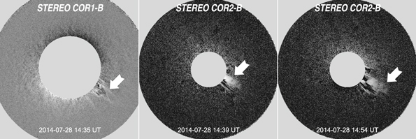
Figure 8. STEREO-B running-difference images taken by COR-1 (left panel) and COR-2 (middle and right panels) during event 11. The initial configuration of this CME showed a narrow jet-like structure (arrow in the left panel) that only developed into a broad CME at high altitudes (when the leading edge of the initial jet was already at ≳4 R⊙) as indicated by the arrow in the right panel.
Download figure:
Standard image High-resolution imageTherefore, we believe that the CMEs in events 10 and 11 evolved from a narrow jet-like structure at low altitudes into a CME at higher altitudes and were only able to drive a strong shock just in the direction aligned with the initial jet. Panels (10) and (11) in Figure 3 show that STEREO-A and STEREO-B in event 10 and STEREO-B in event 11 observed near-relativistic electron and ∼5 MeV proton enhancements associated with these events (for event 11 there is also a later contribution from an SIR on day 211). As shown in panels (10) and (11) of Figure 4, these spacecraft were reasonably well connected to the eruption sites. Given that any shocks present were likely narrow, it is possible that the near-relativistic electrons resulted from the initial jet-like eruption rather than from a well-developed CME shock. For example, in event 10, the SEPT-A ∼45 keV electron onset occurred at ∼15:36 UT, and therefore these electrons were emitted at the Sun when the CME was still a jet (Figure 7) . The fact that only low-energy (<6 MeV) protons were detected by STEREO-A and STEREO-B in event 10 and by STEREO-B in event 11 (panels (10) and (11) in Figure 3) suggests that neither the shock, as it expanded to high altitudes, nor the jet were able to produce higher-energy protons in agreement with Kahler et al. (2019).
The CME in event 2 was generated by a DSF that broke into two well-differentiated structures. Whereas the southern portion erupted rapidly, the portion closer to the equator evolved much more slowly. This evolution resulted in a CME formed by two structures as shown in Figure 9. The southern portion (identified with the arrow in Figure 9) moved at larger speeds. In fact, the speed Vcdaw = 1102 km s−1 listed in the LASCO CDAW catalog is estimated using the southern portion, whereas the portion identified by the solid red line in Figure 9 (originating from the slower and later equatorial portion of the DSF) moved only at ∼690 km s−1 as determined using the three spacecraft points of view (Column (5), Table 1). However, the angular width listed in the LASCO CDAW catalog ωcdaw = 140° includes both structures. Therefore, either structure alone would not have met our criteria for a fast and wide CME. In addition, the portion that intercepted the field lines connecting to SOHO and STEREO-A (both lying close to the equator as modeled by Predictive Science Inc. for Carrington rotation 2108 in www.predsci.com/hmi/spacecraft_mapping.php) was much slower and would have not met our requirements to be included in this study.
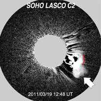
Figure 9. SOHO/LASCO/C2 difference image during event 2 showing a CME with two different structures. The CDAW speed was estimated using the southern structure indicated by the white arrow, whereas the angular width was estimated combining the two well-differentiated structures.
Download figure:
Standard image High-resolution image5. Lack of Magnetic Field Connection
The arrival of energetic particles at a given spacecraft depends on their transport conditions through the corona and interplanetary medium. In the absence of cross-field transport processes, energetic particles propagate through the inner heliosphere guided by the IMF. Hence, the arrival of SEPs at a given spacecraft requires magnetic connection to be established between the particle sources and the spacecraft. The distribution of STEREO-A, STEREO-B, and SOHO during these events (Figure 4) assures us that, in most cases, at least one spacecraft was fairly well connected to the particle sources (assumed to be indicated by the solar event locations) at least along nominal Parker spiral IMF lines. The poorest connection between the parent solar eruption and the nominal footpoint of any of the three spacecraft occurred in events 3 and 5 (see Figure 4). Whereas the absence of >20 MeV protons in these events might be due to this poor connection, the fact that STEREO-B detected low-energy (∼4 MeV) proton enhancements in event 3 and even near-relativistic electrons in event 5 above an already pre-event elevated background (Figure 2) suggests that the source rather than the magnetic connection played a factor in the absence of >20 MeV protons.
The presence of ICMEs, SIRs and/or rarefaction regions in the inner heliosphere at the time when these CMEs occurred might have distorted the estimated nominal connections shown in Figure 4 and therefore affected the conditions for SEP transport from their source to the spacecraft. This is most clearly seen in the case of event 9, which occurred when STEREO-A, STEREO-B, and near-Earth spacecraft were immersed in ICME structures identified using in situ solar wind observations. Figure 10 shows, from top to bottom, ∼2 MeV proton intensities, magnetic field magnitude, magnetic field angular directions in the RTN coordinate system, and solar wind speed, as measured, from left to right, by STEREO-B, ACE, and STEREO-A. The solid vertical lines indicate the passage of interplanetary shocks, and the shaded gray bars denote the passage of ICMEs easily identifiable by the magnetic field smooth rotations (other in situ ICME signatures, as described by Zurbuchen & Richardson 2006, used to identify these structures as ICMEs can be found in www.srl.caltech.edu/ACE/ASC/DATA/level3/icmetable2.html and https://stereo-ssc.nascom.nasa.gov/data/ins_data/impact/level3/). The ICMEs at STEREO-B and Earth are typical "magnetic clouds" with enhanced magnetic fields that rotate through a large angle. The ICME at STEREO-A is much briefer. The purple arrows in Figure 10 indicate the time of the CME 9. Prior to this CME, low-energy particle intensities at the three spacecraft were already elevated owing to prior SEP events. When CME 9 occurred, ACE was immersed in an ICME, and STEREO-A and STEREO-B were in the sheath region formed between the ICME and the shock driven by the ICME. The detection of an SEP event onset is usually impeded when the observing spacecraft is within or close to such structures (Lario & Karelitz 2014). The exception is when the particles are injected directly into the ICME (Richardson & Cane 1996). The ICME detected by STEREO-B on days 102–105 and by STEREO-A on day 102 most likely left the Sun at ∼22:50 UT on day 98 (2014 April 8) from an active region unrelated to the region that generated CME 9. Similarly, the ICME observed near Earth on days 101–102 could not have originated from the region at the east limb that generated CME 9. Therefore, even if CME 9 did accelerate SEPs, as possibly indicated by the long-duration ∼1 MHz type III emission, their access into these ICMEs may have been restricted, and hence they might not have been able to reach any of the three spacecraft.

Figure 10. From left to right, STEREO-B, ACE, and STEREO-A observations during event 9. From top to bottom, (a) ∼2 MeV proton observations as measured by SEPT on STEREO and EPAM on ACE, (b) magnetic field magnitude, (c) magnetic field polar angle, (d) magnetic field azimuthal angle in the RTN coordinate system as measured by the magnetometer experiments on board STEREO (Acuña et al. 2008) and on ACE (Smith et al. 1998), (e) solar wind speed as measured by PLASTIC on STEREO (Galvin et al. 2008) and SWEPAM on ACE (McComas et al. 1998). The solid vertical lines indicate the passage of interplanetary shocks and the gray bands the passage of ICMEs.
Download figure:
Standard image High-resolution image6. Shock Mach Number and Interplanetary Events
Kouloumvakos et al. (2019) found a statistical correlation between the >20 MeV proton peak intensity in large SEP events and the Alfvén Mach number of the shocks in the corona (see their Figure 6). If this correlation holds also for our events, we should expect low Alfvén Mach numbers at the points of the shock front that magnetically connect with each spacecraft (also known as the cobpoint [Connecting-with-the-OBserver-POINT] after Heras et al. 1995). In general, EUV and WL coronagraph images allow identification of the outermost front of the CME, which is usually interpreted as an indication of a shock wave propagating ahead of the CME. Whereas the envelope encircling the outermost front of the CME seems to arise from a driven wave (or shock) close to the CME nose, it may gradually become a freely propagating fast magnetosonic wave at the flanks of the CME (Kwon & Vourlidas 2017). In order to estimate the Alfvén Mach number of these wave fronts around the structure initially driven by the CME, we use the technique developed in Lario et al. (2016, 2017b), which is similar to that used by Kouloumvakos et al. (2019, and references therein). It first uses sequences of EUV and WL coronagraph observations from three points of view (provided by STEREO-A, STEREO-B, and near-Earth spacecraft) to fit the large-scale structure of the outermost front of the CME (Kwon et al. 2014). The fitted geometric shape (either a sphere or an ellipsoid) allows us to estimate the normal to the surface ( ) encompassing the CME front. A sequence of images taken at consecutive times allows us to analyze the evolution of the fitted geometrical shape at any point and hence estimate its speed Vsh along its normal direction. Because of the field of view of the STEREO coronagraphs, the tracking of this structure is done up to distances below 15 R⊙. It is important to emphasize that the geometric shape used to fit the outermost front of the CME is an approximation to the actual front seen in the series of EUV and WL images taken from three vantage points. A compromise between the observed large-scale structure including distortions and corrugations and the geometrical shape is made.
In order to characterize the coronal medium where these structures propagate, we use the results of MHD simulations of the corona. In particular, we use 3D MHD simulations developed by Predictive Science, Inc., in the context of the the Magnetohydrodynamic Around a Sphere (MAS) model in its thermodynamic version (Lionello et al. 2009). This model reproduces the global plasma density and temperature of the corona with sufficient accuracy to recreate many of the multispectral properties of the corona observed in EUV and X-ray emissions (e.g., Riley et al. 2011). These simulations are based on specific Carrington rotations and use photospheric magnetic field synoptic maps built up from a sequence of magnetogram observations centered at central meridian over a 27-day period. In particular, we use the results built from magnetograms collected by the Helioseismic and Magnetic Imager (HMI) on board SDO (Scherrer et al. 2012). Whereas these MHD simulations of the corona are run out to steady-state solutions representative of the whole Carrington rotation, the converging solution may differ from the actual state of the corona at the time when the parent solar eruption takes place, especially for those portions of the corona using old magnetogram observations as input.
The results of the MAS model are considered as representative of the medium that the traveling wave finds upstream as it expands. In particular, we use the solar wind speed  , the magnetic field
  , and the density ρ provided by the MHD model to compute the Alfvén speed VA =
  (where μ0 is the magnetic permeability). We determine the normal
  and the speed Vsh of the large-scale structure used to fit the outermost envelope of the CME all along its front, and hence we compute the Alfvenic Mach number as MA =
  . Note that when the structure propagates into regions of low Alfvén speed (as expected close to the neutral line where
  ), the Mach number acquires large values. It is well known that MHD models tend to provide magnetic fields that are weak when compared to in situ interplanetary observations (e.g., Linker et al. 2017). Kouloumvakos et al. (2019) adopted correction factors to scale up the coronal magnetic field provided by the MHD models, as well as a correction factor to scale down the density values provided by the MHD models. In order to find these correction factors, the averaged values of the unsigned radial component of the MHD magnetic field and solar wind density at an outer boundary within the MHD model are extrapolated using an inverse square dependence and compared with in situ measurements at 1 au. Kouloumvakos et al. (2019) found that the factors to scale up the magnetic field vary from ∼1.6 to ∼2.4, whereas the correction factors for the density vary from ∼0.30 to ∼0.63. Since VA is proportional to B and inversely proportional to the square root of ρ, the correction of magnetic field dominates over the density correction, having a global effect of decreasing the computed Mach numbers of the shock. We have followed the same technique to evaluate the correction factor and scale down the computed values of MA.
Figure 11 shows the distribution of Alfvén Mach numbers over the fitted structures for events 3, 4, 5, 7, 8, and ⊕ at the times indicated in the respective panels. We have excluded from this analysis events 10 and 11 because of their dissimilar evolution from low to high altitudes (Figures 7 and 8), event 2 because of its irregular shape (Figure 9), event 6 where EUV and WL images did not allow the identification of a front wave separated from the body of the CME, and event 9 where even if SEPs were produced their access to the spacecraft was restricted (Section 5). For consistency, we have excluded from Figure 11 event 1 where the MHD background was computed using both magnetograms from the Global Oscillation Network Group and the polytropic version of the MAS model rather than the SDO/HMI data and the thermodynamic version of the MAS model used for the other events (although we have also computed MA for this specific event). The reference point of view in each panel of Figure 11 is the radial direction from the indicated spacecraft. Figure 11 shows that, in contrast to the control event ⊕, where high Mach numbers occupy a large fraction of the surface (for a comparison see also Figure 3 in Kouloumvakos et al. 2019), the high-MA regions in the other selected events are much more limited in extent and correspond to regions of lower Alfvén speed that map back to the neutral line where  (Rouillard et al. 2016). Note that the dark-red regions may indicate MA values well above 4, where color bar saturates.
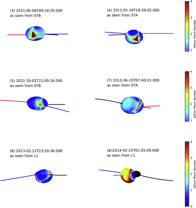
Figure 11. Distribution of Alfvén Mach numbers (MA) over the fitted surface for events 3, 4, 5, 7, 8, and ⊕, at the indicated time and as seen radially from the indicated spacecraft. Blue, black, and red lines indicate the IMF lines connecting to STEREO-B, L1, and STEREO-A, respectively.
Download figure:
Standard image High-resolution imageIMF lines connecting to STEREO-A, L1, and STEREO-B are plotted in Figure 11 using red, black, and blue lines, respectively. These field lines are computed by using the solar wind speed measured by each spacecraft at the time of the CME eruption to ballistically track a nominal Parker spiral IMF line to a heliocentric distance of 30 R⊙, which then connects with the MAS model coronal field that is used to map back the field line to the solar surface or to the fitted surface if magnetic connection with the evolving structure is established. Figure 12 shows the evolution of the speed Vsh (top panel) and Alfvén Mach number MA (bottom panel) for events 1, 3, 4, 5, 7, 8, and ⊕. In panels (a) we show, for each event, the speed at the leading edge of the fitted structure (defined as the point with the highest altitude) and the speed at the cobpoints of those spacecraft that establish magnetic connection with the evolving structure (orange trace for the leading edge, blue for STEREO-B, red for STEREO-A, and black for L1). We omit those spacecraft that, throughout the time we track the outward-propagating structure, do not establish direct magnetic connection with it. The abscissa in Figure 12 is the radial distance above the solar photosphere of the structure leading edge or the cobpoints of each spacecraft. Note that the leading-edge speeds obtained from this fitting for the events shown are consistent with the selection criterion based on Vcdaw of at least 1000 km s−1. As expected, the speed at the cobpoints is slower than at the leading edge. By definition, the leading-edge speed profile may start at a larger distance than the profiles for the cobpoint speeds (which start at the distance where the spacecraft establishes magnetic connection with the evolving structure).
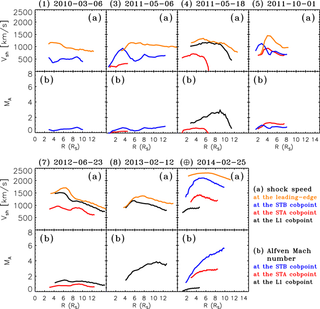
Figure 12. Evolution of (a) the speed Vsh and (b) the Alfvén Mach number MA at the cobpoint of those spacecraft that establish magnetic connection to the fitted structure for events 1, 3, 4, 5, 7, 8, and ⊕ as a function of the cobpoint radial distance above the solar surface. Blue, black, and red lines indicate the parameter at the cobpoint of STEREO-B, L1, and STEREO-A, respectively. Orange traces in panels (a) indicate the speed at the leading edge of the fitted structure.
Download figure:
Standard image High-resolution imageIn panels (b) of Figure 12 we plot MA as a function of the cobpoint radial distance above the solar photosphere for those spacecraft that establish magnetic connection. With the exception of the L1 cobpoint for events 4 and 8, MA is low (≲2) in all the cases. By comparison, in event ⊕, MA at the cobpoints of STEREO-B and STEREO-A acquire large values. As shown in Figure 11, apart from the control event with SEPs, the high-MA regions were limited to narrow areas. Occasionally a spacecraft may establish magnetic connection to one of these narrow high-MA regions such as the L1 observers in events 4 and 8 (as shown by the region intercepted by the black IMF lines in panels (4) and (8) in Figure 11). Therefore, according to the relation between MA and the >20 MeV proton peak intensity inferred by Kouloumvakos et al. (2019), we might expect >20 MeV proton intensity increases at L1 in events 4 and 8, but neither of these two events showed intensity increases.
Lario et al. (2017b) describe in detail the approximations made in this type of analysis. In particular, assumptions include the following: (1) the large-scale structure of the outermost front of the CME can be sequentially fitted with an ellipsoid that approximately expands in a self-similar fashion with time, (2) the background coronal field through which the structure propagates is well represented by a steady-state medium representative of a whole Carrington rotation period, and (3) the magnetic connection to each spacecraft is well described by a nominal Parker spiral IMF line at least up to 30 R⊙ and then traced back to the Sun assuming that the MAS model provides a faithful representation of the field lines in the corona, especially for those regions near neutral lines where MA may acquire large values. As already noted, this last assumption is questionable for L1 during event 4, where the field was radial in a rarefaction region, and for event 9, where ICMEs were present at all locations. In event 8, the presence of an ICME observed at L1 between 17:00 UT on 2013 February 13 and 14:00 UT on 2013 February 16 (www.srl.caltech.edu/ACE/ASC/DATA/level3/icmetable2.html) might very well have distorted the magnetic connection to L1 at the time of the selected CMEs and therefore modified the computed magnetic connection. Similarly, the presence of intervening SIRs might alter the assumed IMF configuration (see Section 6.1 below).
Returning to Figure 12, panels (a) show the evolution of Vsh at the leading edge (orange traces). For those events associated with large DSFs (events 7 and 8), Vsh at the leading edge maximizes at distances ≳6 R⊙ above the solar surface. The slow evolution of the shock at lower altitudes has been pointed out as a factor that distinguishes SEP with soft spectra (E , with γ > 4 at proton energies above 13 MeV) from those with hard spectra where the shock attains high speeds early on during the eruption (E
 , with γ ≲ 3 at proton energies above 13 MeV; e.g., Gopalswamy et al. 2016). For events associated with DSFs, CMEs rise slowly with a constant acceleration and shocks form at several solar radii from the Sun, where the magnetic field and density have fallen off significantly, reducing the efficiency of particle acceleration to high energies by the shock (e.g., Gopalswamy et al. 2017). However, Figure 12 shows events such as 1 and 4, where Vsh at the leading edge is already elevated at the time/distance where the speed can first be estimated, and others (e.g., event 5) where high speeds are attained shortly after this time. While a slow evolution of the shock at low altitudes might help to explain the absence of >20 MeV particles for our CMEs, Figure 12 shows that the CME shocks do not evolve in this way, but instead reach high speeds at low altitudes. Thus, within the assumptions made to compute Vsh, its evolution cannot consistently explain the absence of >20 MeV protons for these CMEs, although the explanation of shock formation height may still be valid for faster CMEs and higher-energy particles.
6.1. Interplanetary Particle Events
As suggested by Rouillard et al. (2016), it is possible that just the high-MA regions favor the acceleration of high-energy particles when the shock is still close to the Sun. Figure 11 shows that for events 3, 4, and 5 a high-MA region was well aligned to intercept, after the fitted structure propagates to 1 au, STEREO-B, STEREO-A, and STEREO-B, respectively. For event 7 the high-MA region might tangentially reach STEREO-A. None of these spacecraft established magnetic connection to these high-MA regions when the CME was still close to the Sun (Figure 12), and therefore no prompt component, at least at high energies, was expected to be observed during these events. Under the assumption that these high-MA regions near the nose of the fitted structure are able to accelerate energetic particles as they propagate outward from the Sun, the arrival of these regions at the respective spacecraft might be accompanied by an energetic particle intensity increase. Cane et al. (1990) described these events as pure-interplanetary particle events, that is, events lacking a prompt component produced shortly after the parent solar eruption when the CME is still close to the Sun but having a particle intensity increase associated with the arrival of an interplanetary shock. Lario et al. (1998) successfully modeled these types of events by deducing that the connection to the region of the shock front able to accelerate particles was established shortly before the shock arrival at the spacecraft.
We have checked whether interplanetary shocks were observed in situ by the spacecraft that was closer to the radial alignment with these high-MA regions in events 3, 4, 5, and 7. Figure 13 shows low-energy particle intensities and magnetic field and solar wind measurements taken by STEREO-B, STEREO-A, STEREO-B, and STEREO-A in events 3, 4, 5, and 7 (from left to right). The purple arrow identifies the time of CME on the Sun, and the purple label identifies the longitude of the parent eruption with respect to the observing spacecraft. We have indicated the passage of interplanetary shocks and ICMEs by the solid vertical lines and gray shaded bars, respectively (following identifications in stereo-ssc.nascom.nasa.gov/data/ins_data/impact/level3/). We also indicate with the label SIR the passage of solar wind SIRs as identified in stereo-ssc.nascom.nasa.gov/data/ins_data/impact/level3/.
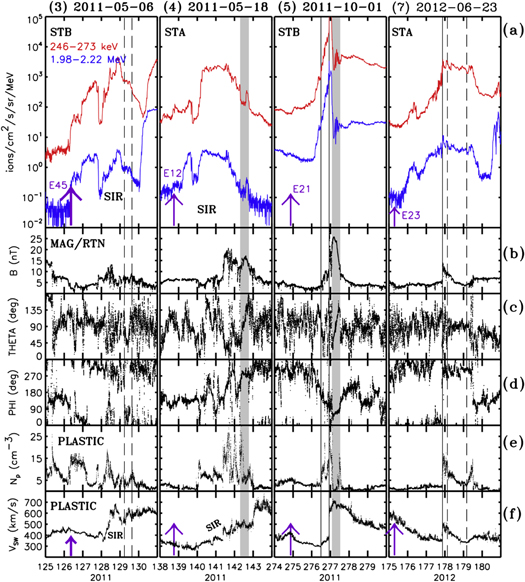
Figure 13. (a) Low-energy proton intensities, (b) magnetic field magnitude, (c) magnetic field elevation angle, and (d) azimuth angle in the spacecraft-centered RTN coordinate system, and (e) proton solar wind density and (f) speed measured by the indicated spacecraft during events 3, 4, 5, and 7 (from left to right). The solid vertical lines indicate the passage of interplanetary shocks, and the gray shaded bars indicate the passage of ICMEs. The vertical dashed lines indicate the passage of sheath structures formed around ICMEs. The purple arrows and numbers indicate the occurrence of the CME and the longitude of the event with respect to the spacecraft, respectively.
Download figure:
Standard image High-resolution imageDuring events 3 and 4, SIRs were present in the interplanetary medium that might have had an effect on the propagation of the CMEs toward STEREO-B and STEREO-A, respectively. In event 3, a short period (∼10 hr) early on day 129 of 2011 (indicated by the two dashed vertical lines in the first column of Figure 13) with a change in magnetic field direction might result from a nearby passage of a flank of the CME embedded within a fast solar wind stream preceded by an SIR observed by STEREO-B early on day 128. No other signatures typical of ICMEs were observed in association with the structure indicated by the two dashed vertical lines. Within the compressed region formed by the preceding SIR, no interplanetary shock was observed. Therefore, we believe that whereas some of the low-energy particles at the onset of the event on day 126 might be due to CME 3, most of the low-energy particles preceding this structure (i.e., on days 128 and 129) were predominantly due to the effects of this SIR, and that the interaction between the CME 3 and the preexisting SIR might have weakened the possible effects of the initial high-MA region before its arrival at 1 au (Pizzo et al. 2015).
In event 4, signatures typical of an ICME (i.e., smooth magnetic field rotation, bidirectional suprathermal electrons, high-charge state solar wind Fe) were observed by STEREO-A for a period of ∼12 hr on day 142 (indicated by the shaded gray vertical bar in the second column of Figure 13). This ICME appeared to have interacted with a high-speed solar wind stream with Vsw already increasing on day 140 before the ICME passage and reaching 700 km s−1 on day 143 after the passage of the ICME. Although a strong compression region was observed prior to the ICME, a shock cannot be identified since increases of different plasma parameters and magnetic field were not coincident. Therefore, we suspect that the low-energy particle increase in event 4 was due to the combined effect of the SIRs and the potential shock driven by the CME that contributed to strengthening and altering the structure of the compressed plasma in front of the SIRs. Nevertheless, this structure was not accompanied by proton intensity enhancements above ∼13 MeV.
Event 5 occurred during the decay of a prior SEP event when low-energy proton intensities at STEREO-B were still elevated but high energies (>20 MeV) were already close to instrumental background levels (panel (5) in Figure 2). A strong shock was observed by STEREO-B at 22:23 UT on day 276 presumably driven by the CME that originated on the Sun at ∼20:48 UT on day 274 and arrived at STEREO-B on day 277 (gray shaded bar in panel (5) of Figure 13). Preceding this shock, a weaker shock was observed at 11:48 UT on day 276 close to a gradual current sheet crossing followed by a gradual increase of B and Vsw. Proton intensities at energies up to ∼25 MeV peaked with the arrival of the strong shock (panel (5) in Figure 2). We suspect that STEREO-B intercepted a strong portion of the shock driven by the CME 5 still efficient in accelerating protons to high energies at its arrival at ∼1 au, although the presence of the preceding weak shock may have favored the confinement of particles upstream of the strong shock and hence the local intensity increase observed at its arrival at 1 au.
In event 7, STEREO-A observed a shock at 20:55 UT on day 177 of 2012. Following this shock, during the first half of day 178 a structure resembling the sheath region of an ICME was observed (indicated by the two dashed vertical lines in the fourth column of Figure 13). This structure was followed by a current sheet crossing on day 179 where the density briefly enhanced. The arrival of the shock on day 177, which may be related to CME 7, coincided with the peak of low-energy proton intensities, but no significant increase was observed at ∼20 MeV energies.
Figure 13 shows that the periods between the occurrence of the CMEs on the Sun and the arrival of the structures related to the passage of the CMEs by ∼1 au in events 3, 4, 5, and 7 were characterized by elevated low-energy (≲5 MeV) proton intensities. By contrast, >20 MeV proton intensities did not show any enhancement during these events (Figures 2 and 3), the exception being the shock on day 277 at STEREO-B in event 5 (panel (5) in Figure 2). The elevated low-energy (≲5 MeV) proton intensities during these events may result from the combined effect of the intervening SIRs and the propagating shocks initially driven by the CMEs that were efficient in proton acceleration at low (≲5 MeV) energies but not at higher (>20 MeV) energies. For example, the low-energy intensity-time profiles in event 7 are typical of an event generated from eastern or central meridian longitudes with a gradual increase peaking with the arrival of the shock (e.g., Cane et al. 1988; Lario et al. 1998). Nevertheless, this event was observed only at low (≲6 MeV) proton energies. For the other events, local interplanetary structures modulated the observed intensity-time profiles.
7. Discussion
Out of the 123 fast (Vcdaw > 1000 km s−1) and wide ( 120°) CMEs reported in the CDAW LASCO catalog from 2009 January 1 to 2014 September 30, in only 11 cases are we certain that the CME did not produce any observable increase of >20 MeV proton intensities at any of the three spacecraft STEREO-A, STEREO-B, or SOHO. Within the Vcdaw–ωcdaw distribution of these 123 events, the 11 selected events were located in the narrower and slower end of the distribution (Figure 1). For a few events the characterization of the CME as wide and fast is misleading because the CME evolves from a jet-like structure at low altitudes that only develops into a wider CME at high altitudes (Figures 7 and 8), or because the CME is formed by multiple structures moving at different speeds and the fastest components of the CME are unlikely to have connected with the spacecraft (Figure 9). The 3D reconstruction of the foremost structure formed in front of the CMEs (using remote-sensing data from the three vantage points that STEREO-A, STEREO-B, and L1 observers provide) results in shock widths ωfit narrower than ωcdaw, whereas the speeds Vfit are similar to Vcdaw (Columns (2) and (5) in Table 1). Therefore, if we had used Vfit and ωfit instead of Vcdaw and ωcdaw, the number of CMEs fulfilling our selection criteria of fast and wide CMEs without production of observable >20 MeV protons would have fallen to just five events. However, because of the wide use of the CDAW LASCO catalog in retrospective SEP studies, we have chosen to use CME parameters from this catalog to select the events.
Several factors may be invoked to explain the nonobservation of >20 MeV protons by any of thee spacecraft. These include the following:
- 1.There was no magnetic connection between the source of the particles and any of the spacecraft.
- 2.There were no particles released at the time of the solar eruption (based on type III radio observations) that could contribute directly to the prompt component of the SEP event and/or provide a seed population for the shock to accelerate.
- 3.A pre-event seed particle population was absent or weak.
- 4.Particle acceleration at either the CME-driven shock (as a whole) or the portion of the CME-driven shock magnetically connected to each spacecraft was not efficient enough to produce >20 MeV protons.
- 5.Accelerated particles were not able to propagate to (or to reach) the spacecraft.
The use of three spacecraft distributed around the Sun during the selected events (see Figure 4) limits the cases where there was no spacecraft magnetically connected close to the presumed region where particle sources are located (i.e., the site of the parent solar eruptions). Among the 11 selected events, the least favorable configuration in terms of magnetic connection between the site of the parent solar eruption and any of the three spacecraft (at least through nominal Parker spiral IMF lines) occurs in events 3 and 5 (panels (3) and (5) in Figure 4) when none of the spacecraft appear to be nominally connected to the site of the parent eruption. However, the development of a fast and, in principle, wide CME assures us that the connection with a potential CME-driven shock might be established by at least one spacecraft. Therefore, the absence of connection to the parent solar eruption does not preclude the observation of SEPs.
Type III radio bursts are thought to be generated by electron beams produced in magnetic reconnection processes (e.g., Cairns et al. 2018). Favorable conditions for high-frequency type III emission are found in high-density regions accelerating intense electron beams. One characteristic of the events selected in the present study is the peculiar radio emissions observed at the time of the CMEs. Figures 5 and 6 show short and weak type III radio emissions at high frequencies that contrast with the intense and long-lasting type III observed in intense SEP events such as in our control event (panel (⊕) in Figure 6). Note also that the DH dynamic spectra in Figures 5 and 6 are from the spacecraft that is front side relative to the solar event, and this therefore excludes the possibility that the weak high-frequency emissions are from a back-side source that is occulted by the limb. The general weak signatures of the type III bursts at high frequencies in our events, together with the short duration of the radio emissions at ∼1 MHz (Column 6 Table 1), indicate that there is only a brief release of electrons at the time of the parent solar eruption. Even for those cases associated with large DSFs, radio emission at high frequencies (≳1 MHz) was absent in events 2 and 8 and very diminished in event 7. Therefore, if particles released during a solar eruption contribute directly to the prompt component of an SEP event, or provide a seed population for subsequent acceleration by the CME-driven shock, the weak type III emissions at >1 MHz during our selected 11 events suggest that such particles were lacking during these solar eruptions.
Figures 5 and 6 show that in events 1, 10, and 11, type III radio bursts persisted at low frequencies for as long as in event ⊕, whereas in the other events radio emissions weakened at much higher frequencies. Weak type III bursts tend to have high stopping frequencies, which could be due to electron beam dilution and/or the effects of background density fluctuations (Leblanc et al. 1995). Although the origin of the near-relativistic electrons and the electron beams generating the type III radio bursts could be different, it is significant that events 1, 10, and 11 clearly showed near-relativistic electron increases at the best magnetically connected spacecraft, as well as low-energy proton increases (see Figures 2 and 3), suggesting a connection between the duration of the type III emission at low frequencies and the arrival of in situ particles (see also Cane & Erickson 2003).
Seed particle populations for the process of particle acceleration by shocks close to the Sun are not directly observable. If pre-event energetic particle intensities are indicative of this seed particle population, we note that events 2, 5, and 9 occurred after sequences of intense SEP events observed by the three spacecraft that globally filled the heliosphere (Richardson et al. 2014). Similarly, events 3, 4, 6, 10, and 11 occurred amid events associated with CIRs (see Figures 2 and 3), which, in principle, sequentially fill regions of the heliosphere with energetic particles, even close to the Sun as recent Parker Solar Probe observations indicate (Allen et al. 2019; Cohen et al. 2019). Therefore, a shortage of seed particle populations close to the Sun cannot be invoked as a factor characterizing those events without a >20 MeV proton prompt component, since the available evidence suggests that, in some events, there was no deficit of seed particles.
It has been suggested that there is a statistical correlation between the >20 MeV proton peak intensity in large SEP events and the Alfvén Mach number of the shocks in the corona at the cobpoint of those spacecraft detecting particles (Kouloumvakos et al. 2019, and references therein). The use of techniques to link the evolution of MA at the coronal shock to the release of SEPs observed by multiple spacecraft distributed in interplanetary space does not always provide successful results (e.g., Lario et al. 2017b), in terms of particles that are estimated to be released before the computed MA exceeds a given threshold. Uncertainties in (i) the extent and speed of the coronal shocks inferred from coronagraph images when using idealized geometric shapes to describe them and (ii) the assumptions made in the MHD models used to both characterize the background where shocks propagate and estimate the magnetic connection between spacecraft and the shocks may be at the origin of these discrepancies. Whereas for our events we deduced low Mach numbers for those spacecraft that establish magnetic connection with our fitted shocks, for two of the events we predicted elevated Mach numbers that do not fit with the general picture (i.e., L1 cobpoints in events 4 and 8; see Figure 12). Similarly, it is worth noting that even in the case of event ⊕, MA at the L1 cobpoint is predicted to be low, when clearly high-energy SEPs were observed at that location (Lario et al. 2017b). Therefore, although statistically it can be found that high-MA shocks are associated with intense SEP events, the exact mechanism that leads to the acceleration of particles to high energies as observed by multiple spacecraft is still dependent on numerous factors that cannot be revealed by current observations. These factors include the properties of the seed particle populations, the presence of upstream plasma turbulence, particle escape conditions from the shock vicinity, and particle release and transport in the interplanetary medium. All these factors play a role in the observation of SEPs after a solar eruption. It has also been suggested that only those portions of the shock that have large MA are responsible for particle acceleration at high energies (Rouillard et al. 2016). In our events, high-MA regions are limited in extent (as compared to those in event ⊕). If these limited regions were able to accelerate >20 MeV protons, then the lack of observations of these particles at any of the three spacecraft locations would appear to place significant constraints on the spreading of particles in the corona and interplanetary medium (e.g., Zhang et al. 2009; Zhang & Zhao 2017).
Finally, the ability of the particles to reach any one of the spacecraft is the ultimate factor that determines whether an SEP event will be observed. The conditions under which particles propagate to a spacecraft are determined by the background medium. The presence of intervening interplanetary structures has clear implications in the observed SEP peak intensities (e.g., Lario & Karelitz 2014, and references therein), and we have discussed how, in the case of event 9 (Figure 10), when the CME might have been expected to be an efficient accelerator of particles, the presence of ICMEs at all three spacecraft could have impeded particle arrival.
8. Conclusions
- 1.We have confirmed that fast (
 1000 km s−1) and wide ( 120°) CMEs tend to be associated with high-energy SEP events, but there is a small percentage of fast and wide CMEs (11 out of 123 events, i.e., ∼9%) without observable >20 MeV protons at the STEREO or near-Earth spacecraft.
 - 2.Within the distribution of fast and wide CMEs, those without >20 MeV proton enhancements tend to be in the narrower end (for our 11 events we found average values of = 1098 km s−1 and = 181°). In terms of mass and kinetic energy, the 11 CMEs without >20 MeV proton events follow the trend of prior statistical studies (e.g., Kahler & Vourlidas 2013) as being less massive and energetic CMEs than those generally associated with SEPs. Therefore, CME dimension and dynamics seem to play a role in the production of SEPs consistent with Kahler et al. (2019). However, the cataloged values of CME widths should be carefully assessed. In particular, the initial evolution of the CMEs should be considered when estimating the relationship between the production of SEPs and the speed and angular width of the CMEs.
- 3.In general, the DH type III radio bursts for those CMEs without >20 MeV protons tend to be weak, in particular at higher frequencies, which suggests that there was little or no particle acceleration/release at the time of the parent solar eruption. The short burst durations at ∼1 MHz are consistent with those found in other studies where no SEP events were observed, and they contrast with the longer-duration and more intense type III bursts that accompany eruptions associated with major SEP events.
- 4.For the CMEs without >20 MeV proton events, the regions of the CME-driven shocks with high Mach numbers tend to be narrow compared to those for CMEs associated with intense widespread SEP events. With a few exceptions and within the approximations used to evaluate spacecraft magnetic field connections and shock Mach numbers, the spacecraft tend to establish magnetic connection with low-MA regions.
- 5.The ultimate factor that determines whether particles arrive is their transport through the corona and interplanetary space. Occasionally, intervening interplanetary structures may have hindered the arrival of SEPs at the nominally well-connected spacecraft, but a full assessment of particle transport conditions for these events is beyond the scope of the present study.


While the extent of the shock front region with high MA is evidently limited, we conclude that the main characteristic that seems to distinguish the fast/wide CMEs that do not generate observable >20 MeV proton enhancements is a deficit in the release of particles at the time of the solar eruption, as evidenced by the weak or absent high-frequency type III radio emissions. The fact that these CMEs also tend to lie toward the lower limits of the speed and width ranges considered in this study (and also mass and kinetic energy) is apparently consistent with statistical studies showing positive correlations between CME speed/width and SEP intensity and suggests that the properties of the CMEs and, presumably, the characteristics of the parent eruption may also play a role in the reduced particle emission. On the other hand, their distributions in Figure 1 overlap with those of CMEs with SEP events; in addition, slower and narrower CMEs than those considered here may be associated with >20 MeV proton events detectable by the STEREO and near-Earth spacecraft (e.g., Richardson et al. 2014, 2015), so the CME parameters alone cannot account for our fast/wide CMEs without proton events. A puzzle that then remains is how these fast/wide CMEs were produced, presumably requiring a substantial energy release, yet the signatures of energetic particle acceleration and release in these events were relatively modest.
Data used in this paper can be downloaded from www.srl.caltech.edu/ACE/ASC/, www2.physik.uni-kiel.de/stereo/, www.srl.caltech.edu/STEREO/, cdaweb.gsfc.nasa.gov. We thank the STEREO: IMPACT, SECCHI, WAVES; SOHO: LASCO, ERNE; Wind/WAVES; and SDO/AIA teams and Predictive Science Inc. for providing the data used in this study. The STEREO SECCHI data are produced by a consortium of RAL (UK), NRL (USA), LMSAL (USA), GSFC (USA), MPS (Germany), CSL (Belgium), IOTA (France), and IAS (France). SOHO is a mission of international cooperation between ESA and NASA. The SDO/AIA data are provided by the Joint Science Operations Center (JSOC) Science Data Processing (SDP). We acknowledge all the science instrument teams for making their data used in this paper available. We acknowledge the use of the LASCO CDAW catalog generated and maintained at the CDAW Data Center by NASA and the Catholic University of America in cooperation with the Naval Research Laboratory. The present work has also benefited from discussions held at the International Space Science Institute (ISSI, Bern, Switzerland) within the frame of the international team High EneRgy sOlar partICle events analysis (HEROIC) led by Dr. A. Papaioannou. The development of the 3D geometric models was supported by the National Research Foundation of Korea (NRF) grant funded by the Korea government (MSIT; project No. 2019-2-850-09). V.K. acknowledges support by an appointment to the NASA postdoctoral program at the NASA Goddard Space Flight Center administered by Universities Space Research Association under contract with NASA and the Czech Science Foundation grant 17-06818Y. D.L. was supported by NASA-HGI grant NNX16AF73G and NASA/LWS grant NNX15AD03G. I.R. acknowledges support from NASA program NH14ZDA001N-LWS. D.L., L.B., M.Z., and I.R. acknowledge the support from the NASA program NNH17ZDA001N-LWS.