
Abstract
Crystalline defects, such as line-like dislocations, play an important role for the performance and reliability of many metallic devices. Their interaction and evolution still poses a multitude of open questions to materials science and materials physics. In-situ transmission electron microscopy (TEM) experiments can provide important insights into how dislocations behave and move. The analysis of individual video frames from such experiments can provide useful insights but is limited by the capabilities of automated identification, digitization, and quantitative extraction of the dislocations as curved objects. The vast amount of data also makes manual annotation very time consuming, thereby limiting the use of deep learning (DL)-based, automated image analysis and segmentation of the dislocation microstructure. In this work, a parametric model for generating synthetic training data for segmentation of dislocations is developed. Even though domain scientists might dismiss synthetic images as artificial, our findings show that they can result in superior performance. Additionally, we propose an enhanced DL method optimized for segmenting overlapping or intersecting dislocation lines. Upon testing this framework on four distinct real datasets, we find that a model trained only on synthetic training data can also yield high-quality results on real images–even more so if the model is further fine-tuned on a few real images. Our approach demonstrates the potential of synthetic data in overcoming the limitations of manual annotation of TEM image data of dislocation microstructure, paving the way for more efficient and accurate analysis of dislocation microstructures. Last but not least, segmenting such thin, curvilinear structures is a task that is ubiquitous in many fields, which makes our method a potential candidate for other applications as well.
Export citation and abstract BibTeX RIS

Original content from this work may be used under the terms of the Creative Commons Attribution 4.0 license. Any further distribution of this work must maintain attribution to the author(s) and the title of the work, journal citation and DOI.
1. Introduction
Crystalline defects play an important role for the performance and reliability of many devices and components and are of big interest in materials science and materials physics. For example, the motion and interaction of dislocations, i.e. linear defects in the crystal lattice of metals or semiconductors, is directly responsible for plastic deformation and thereby has a strong influence on the resulting mechanical properties. Understanding the dynamic behavior of dislocations is therefore of great importance. One way of achieving this is to observe them while they move and interact. In-situ transmission electron microscopy (TEM) allows to do so and is the method of choice for this work.
TEM is the most often used method to directly visualize dislocations. It is based on the interaction of an electron beam with the crystalline specimen in form of a thin foil. Furthermore, in-situ TEM studies allow to simultaneously perform mechanical testing and to capture the motion of such defects as well as their interaction with obstacles, e.g. other dislocations, second phase particles or grain boundaries [1]. 'Quantitative in-situ TEM' frequently refers to the ability of capturing both the evolution of a microstructure through electronic imaging and at the same time to estimate (externally) the associated stress response as demonstrated in a number of studies [2–5]. This could—in principle—also help to understand the structure-property relationship by extracting data from TEM images (see, e.g. the work and discussion in [1]). Lee et al [6] observed the evolution of dislocation plasticity and additionally calculated the shear stress acting on dislocations from the estimation of their line curvature in a high entropy alloy. In all these studies, the stress is only roughly estimated because the local line geometry, i.e. in particular the local curvature, could not be obtained. Steinberger et al [7] manually extracted the position of dislocations and used these as input for finite element simulations to study the local stress state. Utt et al [8] tracked the positions of dislocations over time and observed that they move in a jerky manner, moving by continuous pinning and depinning. While all authors could extract new information from their investigations, only very few TEM images from the whole data could be analyzed as this had to be done manually. Therefore, the statistical scatter from these 'singular data points' is rather large and can make it difficult to capture the entire dynamic process of dislocation motion appropriately.
A prerequisite for analyzing the dynamic behavior of the dislocations is the ability to extract all dislocations as mathematical curves. These can be represented by, e.g. polynomial approximations such that even local geometrical properties can be represented as demonstrated in [9, 10]. Up to date, digitization of dislocations is almost always done manually. This 'hand labeling' was done in the past without a specific software, and only recently dedicated tools such as labelme [11] were used. Dislocations can be annotated as a line by selecting points on the dislocations using these tools. In [10], such a manual method was used to extract the information of dislocations from 300 individual frames where each frame has up to 20 dislocations. This is a challenging and tedious task, difficult to reproduce, and the result may depend on the experience of the person who performs the labeling of the images. The last aspect is a particular challenge as stress calculations can be very sensitive to the local radius of curvature of a point on the line. With detectors and cameras becoming increasingly faster, there is an urgent need to automatize the analysis of the huge amount of image data generated by TEM in general and during in-situ TEM experiments in particular.
Deep learning (DL) based methods can be very powerful tools for performing pixel wise classification to segment objects of interest. This can significantly help to automate the analysis of microscopic images [12–14]. In general, state of the art DL architectures such as the U-Net [15] have been found to be very successful for image segmentation with applications ranging from the classical field of computer vision [16–18] to medical imaging [19–21]. Such models also have been applied to several problems in the field of material science, e.g. to segment nano-particles [22] and even for identifying precipitates, voids and simple dislocation networks [23]. Furthermore, Shen et al [24] used DL-based segmentation to identify small defect loops. While these methods are clearly very useful for analysis of images, they suffer from the problem that they require large amount of training data and/or are not accurate enough to represent dislocations as splines. Usually in this scientific domain, training data is not available and needs to be manually created to obtain the ground truths for a supervised machine learning (ML) task.
An additional challenge specific to segmentation of dislocations from TEM images is the variance of the observed 'dislocation phenomena' along with varying imaging conditions: creating a representative amount of training data that covers all possible configurations requires many experiments. This is very expensive and time consuming; performing experiments that cover rarely observed situations might even be impossible in all generality. A lack of a diverse dataset often leads to over-fitting of the ML model where the already learned images are very well predicted but prediction for micrographs from new experiments are surprisingly bad: thus, the generalization of the trained model to new data/situations is strongly limited. These difficulties are even amplified by the fact that there are no publicly accessible data sets of dislocation microstructures available that could be used to augment the training data set or that could be used in a transfer learning approach.
However, training on small datasets can be possible to some extent: Sasaki et al [13] tried to circumvent the problem of 'never-enough-data' and used the first 100 frames of a TEM video for training and the next 70 images for testing. Unfortunately, no quantitative evaluation of the performance was given; it was difficult to estimate the performance of the trained model on new experimental data since the model is trained on very similar data from the same video. Their emphasize was rather on development of a method for tracking dislocations over several frames. In another study Roberts et al [23] obtained two images of  pixels in size, divided the whole image into five parts and used three of them for training, one for validation and one for testing. Together with basic augmentation operations this resulted in a total training data set of 48 images. The intersection over union (IoU) performance for dislocations was stated as 44%. Nonetheless, care need to be taken when the test data used is very similar to the training data as in such cases the model can again be prone to overfitting.
The lack of high-quality and high-quantity training data can be overcome by generating synthetic images [25, 26]. This is an approach which so far has only been rarely used in the field of materials science [27, 28]. In the context of dislocation microstructures this was not used at all. There are several techniques available to generate synthetic data ranging from domain randomization [29] where non realistic objects are added to force the ML model to learn important features, to ML guided methods such as, e.g. generative adversial networks (GANs) [30] where a ML model learns to generate synthetic data with features similar to real data. Chun et al [31] used a GAN to generate synthetic heterogeneous energetic material microstructures. For image segmentation tasks, it is important to generate the ground truth masks along with the synthetic image. More advanced DL models ranging from text-to-image generative models called 'stable diffusion' [32–34] not only provide high quality synthetic images but also ground truth for segmentation tasks. However, such methods are specific to general images and method cannot be directly used for other cases, such as dislocation microstructure. A different class of approaches for image generation is the use of rendering software such as, e.g. Blender [35]. There, the focus is rather on lightning and rendering of three-dimensional objects, but in principle this can also be used to generate two-dimensional synthetic data. Example applications of very realistically looking images in the context of nanoparticles can be found in [22, 36].
Another possibility in the field of material science is to use simulation methods to create synthetic images [37]. There are—in principle—many methods and models readily available, covering all phenomena from atomistic to macroscopic scales. Such simulations can be used to generate synthetic data as shown by Hajilounezhad et al [38] where a scanning electron microscopy (SEM) simulation tool is used to get artificial images of a carbon nanotube forest along with the calculated properties of the structures used as ground truth. In another study, microstructure representations are generated using simulation models, which are then rendered to obtain simulated images [39]. Trampert et al [27] used Voronoi tessellations to generate synthetic polycrystalline microstructures: even though the statistical properties of the grain size distributions are only roughly comparable to those reported for real grain distributions, the degree of visual similarity and the type of contained features (e.g. triple points) turned out to be sufficient for an effective training process. This demonstrates that synthetic data can be a very useful way of obtaining training data for those cases where no suitable, 'real' microscopy training data is available. However, up to date, there exists no systematic analysis of how to create synthetic training data for TEM images of dislocation microstructures and how to infer which features need to be included and which are superfluous.
In this work, we propose a parametric model for generation of synthetic image data of dislocation microstructures. The parameters control (i) various aspects of the microstructure, (ii) details of the background as well as (iii) different types of noise. We show how to choose the parameters that mimic a particular dislocation microstructure and furthermore how to create a simple statistics from sets of real microscopy images that help to model the synthetic microstructure images. Subsequently, a loss function is introduced that considers physics-aspects of the line-like dislocations and that contains a particular emphasize on being able to separate nearby dislocations with sub-pixel accuracy. Thus, the focus of this work is on prediction accuracy, while the aspect of generalization is somewhat less important. Even though, the used DL model is trained only on synthetic data, it turns out that reliable predictions can also be made for real images, which can be further improved by finetuning the model with a very small number of real images.
This work is organized as follows: the parametric model for generating synthetic training data is presented in section 2. The ML model and the physics-informed loss function are described in section 3 while section 3.4 introduces further aspects of the real datasets used for further benchmarking. The results are presented as well as discussed in section 4. Finally, conclusions of the work are presented in section 5.
2. Synthetic data generation model
In the context of microscopy, synthetic data refers to images that mimic the relevant details, i.e. geometrical and imaging features usually found in real microscopy images. Typically, other less relevant details are then neglected, as is the case in any model of reality. Finding out which aspects of TEM images need to be considered and, based on that, how to generate effective synthetic training data is one of the goals of this work.
A parametric model for creating artificial TEM images must satisfy two requirements: (i) create images and masks that are sufficiently similar to real images so that once a ML model is trained on the synthetic training data, it can also provide high quality results on real images, and (ii) use as few parameters as possible to describe the details of the image. The first requirement is obvious while the second is important for easily adapting the parametric model to other TEM experiments or materials and thereby to enhance generalization in situations beyond the single experiment. Creating a synthetic image of a dislocation microstructure consists of three concrete steps:
- 1.Generating a background for the synthetic image: two fundamentally different approaches are used in this work. The first approach is entirely artificial and superimposes different types of noise and smoothing operations. The second approach uses background image patches from real microscopy images.
- 2.Generating the geometry of the artificial dislocation microstructure: in this step, the position and geometrical shape of the dislocations and possibly other elements are determined.
- 3.'Drawing': the process involves rendering the dislocations on the background, writing the image and mask as a PNG file, and recording all parameters in a JavaScript Object Notation (JSON) file to ensure full reproducibility.
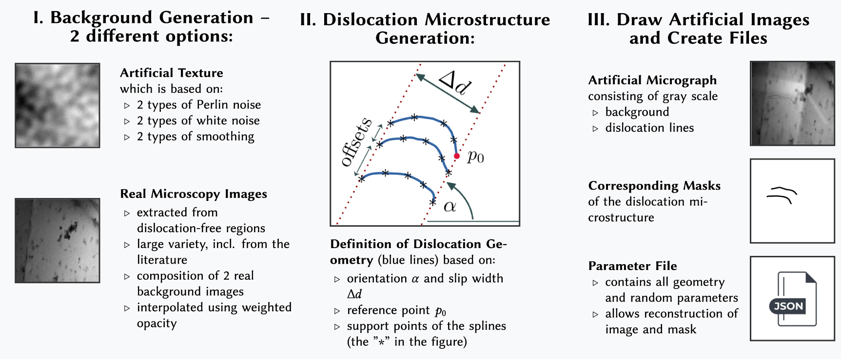
An overview of these steps together with a list of the most important parameters are shown in figure 1. In the sections that follow, all steps and the involved parameters will be explained.

Figure 1. Synthetic images and masks are generated in three steps. First, a background image is created from artificial 'noise generators', or by using background images from real microscopy data Then, the dislocation geometry is determined and subsequently 'drawn' on top of the background providing the synthetic image, mask as well as the parameter file.
Download figure:
Standard image High-resolution image2.1. A purely synthetic approach to background generation
Noise, randomness and a well-chosen variance of different features in the training dataset are key ingredients for a good training process; they reduce the risk of overfitting and are also helpful for generalization of the model to new images. Therefore, the generation of suitable background textures was an important task. For this purpose, we analyzed a number of real microscopy images and found that very often a number of different gray value gradients (e.g. owing to the microscopy imaging conditions) as well as random fluctuations in the brightness occurs. E.g., these may be due to random 'dirt' particles on the surface of the specimen or also due to the presence of other defects that are either not visible or only barely visible due to the diffraction condition.
We use two-dimensional Perlin noise which has been widely used to create texture for computer games [40–42] because the structure is natural looking and can be designed such that it does not repeat itself within the image. The algorithm of Perlin noise uses random gradients on regular grid points of two-dimensional domain along with interpolations to generate random noise of a particular main wavelength. The Python implementation from [43] was used for this work. Perlin noise does not exactly look like the backgrounds of real TEM images as can be seen in the examples in figure 2, and hence may not exhibit the same statistical properties as the background of real images, e.g. in terms of brightness distribution or the spectrum of wavelengths. However, it offers an effective way of introducing a non-trivial type of randomness (as opposed to, e.g. white noise). As a default, we use a superposition of Perlin noise with two different wavelengths where the larger wavelength is motivated by the mild gradient of gray value changes that encompasses the whole TEM image, e.g. due to the imaging conditions. The smaller wavelength represents all other fluctuations. Additionally, we applied a sequence of white noise followed by a Gaussian filter twice with different parameters.

Figure 2. The rows show four examples for synthetically created background images. The most important steps of the background creation pipeline together with the used parameters are shown from left to right.
Download figure:
Standard image High-resolution imageTo mathematically formulate the subsequent steps, we introduce an image with M × N pixels as a function I that maps each discrete pair of pixel coordinates,  to a gray scale intensity that can take values within the unit interval
 ![$[0,1]\subset \mathbb{R}$](https://content.cld.iop.org/journals/2632-2153/5/1/015006/revision2/mlstad1a4eieqn3.gif) ,
,


where (m, n) denotes an individual pixel with the intensity  . Similarly, any image operation T is a function that maps the value of each pixel
  of an image to a new value
  . By chaining such functions, one can also perform several subsequent operations on and with images. For the problem at hand, we start with two image generating functions each of which results in an image with Perlin noise, P1 and P2. Structural details of the Perlin noise image depend on the wavelength parameter λ1 and λ2. A new image P3 is obtained by adding the corresponding pixel values of two images and additional weighting P2 with a factor
  , resulting in

Subsequently, the value range is scaled to the unit range by the following operation:

where  and
and  denote the minimum and maximum pixel value of an image P, respectively. In the next step, an image X1 which contains white noise is added. It is obtained by sampling each pixel value from a uniform random distribution with values in between 1 and −1. The values of X1 are then weighted with
  and superimposed with the previous data to obtain

The resultant is then (usually: only slightly) smoothed using a convolution with a discrete Gaussian filter kernel that has standard deviation s1. This smoothing function G1 then results in the image P5:

The operations resulting in P4 and P5 lead to slightly 'smeared out' random fluctuations which might, e.g. stem from the noise of the microscope electron optics or the camera noise. We then add additional white noise X2 weighted by the standard deviation of the values of P4, i.e.  , and apply one more Gaussian filter G2 with standard deviation s2 to adjust the width of these spikes,


Due to the scaling of this final white noise, P7 might also contain negative values. Along with a 'clipping' of the data to the range of ![$[0,1]$](https://content.cld.iop.org/journals/2632-2153/5/1/015006/revision2/mlstad1a4eieqn12.gif) this gives the final background image P:
this gives the final background image P:

Adding the noise X2 together with the smoothing of G2 only slightly changes the image but in conjunction with the clipping, gives sharper, high frequency fluctuations. The combination of the two noise types X1 and X2 and the smoothing operations G1 and G2 is also a way to mimic artifacts from the usually lossy image compression often used in proprietary microscopy software.
Our studies show that the two types of Perlin noise together with some high frequency oscillations are the most effective contributions for a high quality training dataset; even a single white noise contribution often suffices. To increase the variance of the dataset, we nonetheless kept both the white noise contributions together with the subsequent smoothing operations. In figure 2 we show some examples for intermediate steps and the final background together with the respective parameters. The images have a resolution of  pixels. In the first two examples, only the wavelengths of the Perlin noise contributions are varied. There, it can be observed that textures with very different characteristics can be reproduced. Some of them resemble backgrounds of real microscopy images, but not all of them do. Below, we will also investigate the importance of having a high degree of realism. All parameters as well as the seeds for the random number generators were recorded and stored in a JSON file so that the synthetic background could be fully reconstructed.
2.2. Background generation using real images
The second approach for generating background images utilizes real images and is aimed at producing highly realistic background textures. To achieve this, we collected 170 TEM images featuring dislocation microstructures, specifically focusing on larger regions devoid of dislocations. These 'background-only' patches were then carefully cropped and manually extracted. The images were obtained from a diverse range of sources, including an extensive body of existing literature. It is important to note that we did not use any backgrounds from the four real datasets employed in this study. To enhance the diversity of the data, two background images were chosen at random and superimposed with a random opacity value. Although the resulting image may appear somewhat unusual or even 'incorrect' to an expert observer, the presence of additional background features has proven to be beneficial for the generalization of the ML model when applied to real data. In order to ensure the reproducibility of this background generation process, we documented all parameters of the individual images, as well as the opacity parameter used during the superimposition process. This documentation enables other researchers to replicate our methodology and further explore our findings in their own scientific investigations.
2.3. Generation of artificial dislocation microstructure
Dislocation structures in TEM images exhibit significant variations in terms of shapes, relative sizes with respect to the image dimensions, the number of active slip systems or the orientations of dislocations (some of such examples are shown in figure 5). Throughout this work, we mainly consider dislocations in so-called pileup configurations (this denotes nearby dislocations that strongly interact with each other and often move approximately simultaneous). The special case of a single dislocation is contained as a pileup having only one dislocation. When dislocations move, they create so-called slip traces, corresponding to the interception of the glide plane of these dislocations with the free surfaces of the thin foil [44]. In in-situ TEM experiments, they appear as weakly contrasted, either dark or light, straight lines that should be ignored by the DL model. The slip traces are characterized by the angle of inclination, α, and by the slip width  as shown in figure 1 and are used for determining the dislocations' positions.
A dislocation starts at one of the slip traces and ends at the other slip trace line, as shown in figure 1(II). The start point of the first dislocation in a group (pileup) of dislocations is given by the parameter p0. Here, the dislocation line is mathematically represented as cubic spline, and the geometrical shape of the line is governed by a number of support points. These support points can be obtained either from the labeling of dislocations in real TEM images using e.g. the software tool labelme [11], or by prescribing some reasonably looking coordinates (e.g. by randomly choosing an average curvature and then adding random variations to each of the support points). Subsequent dislocation in a group can then be obtained by shifting the first dislocations' support points along the slip traces by an offset value, followed by adding some randomness to the final line shape or by prescribing a new set of support points as before. A single real microscopy image may contain several groups of dislocations that might move in different directions. This can be realized by repeating all the above steps, starting with determining the slip traces. Again, we record all the parameters used as well as the seed values for the random number generator and store them in a JSON file.
As a final step, we use the Python package Matplotlib [45] to draw the dislocations on top of the respective background. Each dislocation line has a gray value and a line thickness assigned, both of which are randomly chosen from a range of reasonable values. Also, we ensure that the dislocation appears slightly darker than the background, as is also the case in real images figure 5). While drawing the gray dislocation lines on the background we also draw the dislocation lines as solid black lines on an empty canvas as ground truth for the segmentation task. For ease of future reference and exact reproducibility, we record all pertinent parameters in a JSON file.
For the here investigated situations and image sizes, we find that the total time required to generate a synthetic image varies linearly with the total number of dislocations present in the image. On a regular workstation it takes on average about 6.3 s to generate a synthetic image that contains 10 dislocations. This results from approx. 0.6 s for a single dislocation and 0.1 s for creating the background consisting of two images or 0.2 s for creating the background consisting of Perlin noise. The dependency on the number of supporting points of the spline is negligible.
2.4. Properties of synthetic images
The objective of using synthetic images is not to have images that exactly replicate the physical properties of actual dislocation microstructures. In some instances, they might even slightly contradict physical laws (e.g. a certain local dislocation curvature might be impossible to be encountered in reality). We performed a preliminary study, in which it turned out, that such 'nonphysical perturbations' do not have a negative influence on the training performance; sometimes, the inclusion of nonphysical details was even helpful since it increased the overall variance in the image dataset. Thus, the paramount concern is to ensure that the synthetic images are sufficiently rich in terms of parameters and features, enabling to generalize across all relevant dislocation structures. Some examples of these synthetic images are shown in figure 3.

Figure 3. Some of the wide range of synthetic images that can be generated by different values of the parameters.
Download figure:
Standard image High-resolution imageThis synthetic data generation approach can also be easily modified for object detection, instance segmentation, or classification tasks related to dislocation microstructures by generating the respective ground truths. As a parametric method, it also has the advantage that it can synthesize rarely encountered microstructures. While this work focuses on specific dislocation microstructures, the parametric model can also be adapted to other line-like shapes. One of such examples is x-ray-based imaging of bubble formation during additive manufacturing [46], where bubbles can be represented as ellipses, polygons, or splines. Another potential application is the detection of biological worms [47, 48], offering a versatile approach to obtain training data especially in cases where no ground truth for real data is available.
3. Learning strategy
The goal of the next steps is to segment dislocations such that each of them can be represented as a mathematical spline. This enables us to perform quantitative calculations, such as computing the velocity, position, and curvature, as demonstrated in [10]. Training a ML model for segmentation tasks can be challenging, in particular when dislocations are nearly touching each other (see, e.g. figures 5(a) and (c)) or even overlap.
3.1. ML model
To address this challenge, we present a methodology designed to predict individual dislocations as distinct masks. Each mask represents a single dislocation, ensuring that all pixels within that mask correspond to the same dislocation. For this, a U-Net++ with a ResNet50 backbone was used [49], implemented using the PyTorch library. Indicated by a preliminary study, this architecture strikes a good compromise between accuracy and computational efficiency, even though more advanced architectures exist. Note, that benchmarking network architectures is not the focus of this work, rather, the goal is to investigate the performance of synthetic training data as a substitute for real training data.
The input to our model are images with  pixel in size, and the output is a set of masks with dimensions
  pixels, where N represents the maximum estimated number of dislocations within an image. In the examined real images used in this study, we have chosen N to be 20 which will allow the model to predict a maximum of 20 masks, each corresponding to one of the 20 dislocations.
We now explore a first segmentation example. A synthetic image, along with the corresponding masks, is depicted in figure 4. This image considers a dislocation pile-up of five dislocations, shown as ground truth mask numbered from 1 to 5 (top row). Ideally, one would expect that the ML model should predict the five dislocations in five individual masks, and the remaining 15 predictions should be empty masks. However, for simplicity, this is not enforced, and we also allow that these masks may contain dislocations. In that case, any duplicate dislocation can be easily filtered out in a subsequent post-processing step.

Figure 4. A synthetic image of a dislocation microstructure with five dislocations. Top row: each dislocation is contained in its own ground truth mask; adding them up results in the mask of the full dislocation structure. Bottom: predictions using 20 masks.
Download figure:
Standard image High-resolution image3.2. A loss function tailored to dislocations
Training the model to predict only one dislocation per mask, we propose a novel loss function which, at the core, is based on the widely-used Dice loss [50]. The Dice loss is calculated as

where  (True Positives) is the number of pixel correctly predicted as part of a dislocation,
  (False Positives) is the number of pixel incorrectly predicted as part of a dislocation,
  (False Negatives) is the number of dislocation pixels that were missed. Our loss function is based on the fact that each ground truth mask contains exactly one dislocation. The number of possible masks for the prediction is a parameter that is specific to the microscopy situation and that needs to be equal or larger than the number of dislocations in the image (usually, it is easy to determine, if the material scientific experiment considers 2 or 20 dislocations). Figure 4 also shows an additional aspect of the prediction of multiple masks: e.g. the predicted dislocation number 1 does not necessarily corresponds to ground truth mask number 1. Hence an important step is to find for each dislocation the most suitable mask. This is done by calculating the Dice loss for all combination of true masks and predicted masks. For a specific dislocation (i.e. true mask), the corresponding predicted mask with the lowest Dice score is chosen as the most suitable prediction. This approach is presented in algorithm 1.
| Algorithm 1. Compute average image loss for all dislocations. |
|---|
 true_masks
 list of ground truth masks, e.g. the ith mask is true_masks[i] list of ground truth masks, e.g. the ith mask is true_masks[i]
|
 pred_masks
 list of predicted masks, e.g. the jth mask is pred_masks[j] list of predicted masks, e.g. the jth mask is pred_masks[j]
|
| 1: function ComputeAverageLoss(true_masks, pred_masks) |
2: M
 number of elements in the list true_masks number of elements in the list true_masks
|
3: avg_loss

|
4:  Iterate through all ground truth masks and find the best, predicted mask for each Iterate through all ground truth masks and find the best, predicted mask for each |
5: for
i
 1, M
do
1, M
do
|
6:  obtain the loss for all predicted masks and the ground truth mask i obtain the loss for all predicted masks and the ground truth mask i
|
7: N
 number of elements in the list pred_masks number of elements in the list pred_masks
|
8: loss_values

 DiceLoss DiceLoss
![$(\texttt{true}\_\texttt{masks[i]},\, \texttt{pred}\_\texttt{masks[1]}),$](https://content.cld.iop.org/journals/2632-2153/5/1/015006/revision2/mlstad1a4eieqn32.gif)
|

|
DiceLoss
![$(\texttt{true}\_\texttt{masks[i]},\, \texttt{pred}\_\texttt{masks[N]})\big]$](https://content.cld.iop.org/journals/2632-2153/5/1/015006/revision2/mlstad1a4eieqn34.gif)
|
9:  find the index of the predicted mask with the lowest loss value find the index of the predicted mask with the lowest loss value |
10: idx

|
11:  update the resulting loss of the image, given that there are M masks update the resulting loss of the image, given that there are M masks |
12: avg_loss
 avg_loss + loss_values[idx]/M
|
13: 
 and exclude the predicted mask to avoid double counting: and exclude the predicted mask to avoid double counting: |
| 14: remove the mask at index idx from list pred_masks |
| 15: |
| 16: return avg_loss |
Once the mask for each dislocation in an image was found, post-processing steps are performed for representing dislocations as mathematical splines. A metric for evaluating the performance of the overall prediction can then be calculated, based on the line lengths of the fitted splines:
- 1.Binarization of the predicted mask: convert the predicted mask into a binary format (0 for background and 1 for dislocation) using a threshold of 0.5.
- 2.
- 3.Application of Lee skeletonization [53]: employ Lee skeletonization to refine each connected region to a one-pixel thickness, thereby facilitating a cleaner representation of the dislocation.
- 4.Spline fitting: treat the points derived from skeletonization as support points, utilizing them to represent each dislocation as a spline.
- 5.Calculation of metric score: the metric score is determined based on the relative error, i.e. by comparing the length of the predicted dislocation, LP (represented by the spline), with the length of the ground truth dislocation, LT :


A metric value of 1.0 would imply a perfect predicted dislocation length, which generally also implies that the predicted mask aligns precisely with the ground truth. It is important to note that this metric might yield lower scores in case of minor prediction discrepancies. However, in general, it gives a more accurate representation of the model's performance. The reason is, that a pixel-wise metric does not capture the non-local, line-like nature of dislocations. How about adding more geometrical features to the loss, such as the orientation or even the (local) curvature? This might seem like a useful approach since the stress locally acting on a dislocation can depends on such details. However, we found that errors from orientation differences are already indirectly considered in the Dice score since it uses the intersection of the ground truth with the prediction. Therefore, including additional geometric features was not considered any further.
3.3. Training details and the synthetic datasets
We perform training on synthetic datasets with 4000 training images and 1000 images for testing. During training, we try to achieve optimal performance on the synthetic datasets by saving the model that achieves the highest score. Optimal performance is determined using the above introduced physics-based metric, evaluated on the test data. This is a commonly used strategy for preventing overfitting and improving generalization on unseen data [54] which also helps in enhancing the model's robustness. We use a number of image transformation methods during the training process such as applying Gaussian noise, changing brightness, contrast and image equalization to diversify the texture properties of the synthetic images. This improves the model's ability for generalization when applied to real images.
3.4. Real datasets (RD1–4)
For validation purposes (but also for fine tuning) we use data from four in-situ TEM experiments, referred to as RD1–4, to test the ML model trained on synthetic datasets. Individual frames were extracted from the experimental videos, and each experiment produced several thousands of frames, with the position and shape of the dislocations as well as the imaging details being the primary distinction between consecutive frames. These variations in dislocation microstructure can be observed in figure 5, where frames from the same video are shown. On a first glimpse snapshots from the same dataset look relatively similar; however, geometrical details and numbers of dislocations change, and also the camera position and the lightning conditions undergo more or less big changes. Moreover, there are substantial differences between the four datasets.

Figure 5. Three different frames from four real datasets RD1,RD2,RD3 and RD4 (in four columns) obtained from different in-situ TEM experiments.
Download figure:
Standard image High-resolution imageMost of the image sequences are configurations of less than 20 dislocations. One of the challenges encountered was to discriminate between dislocations that can be closer to each other while others are more easily resolved (datasets RD1 and RD3). This scenario can arise when a pile-up is halted by a strong obstacle, or in certain alloys where short-range order may lead to such pairing [55]. Another common challenge is incorrect prediction of a slip trace line as dislocation (as is the case, e.g. in RD3). RD4 poses an extra challenge as it contains a large number of dislocations of varying sizes and shapes each requiring meticulous identification and segmentation.
4. Results and discussion
4.1. Synthetic training data for two different parametrizations
The challenge of determining suitable parameter values for synthetic data generation models results from the need to ensure that a ML model, trained on synthetic images, should also yield satisfactory results when applied to real images. Often, synthetic images do not accurately capture all features, variations and intricacies (such as changing lightning conditions) present in real TEM images. As a result, a ML model optimized for synthetic images may struggle to generalize well to real images. Therefore, it is important to identify the optimal combination of parameters for the synthetic data generation model.
To identify these parameters, 15 hand-labeled images from the RD1 dataset are used to determine the typical value ranges of the number of pileups, the number of dislocations within a pileup, the slip width and slip direction, and the spacing between the two nearest dislocations in a pileup. These value ranges are shown in form of probability density distributions in figure 6 (top row, RD1). The first synthetic dataset used for training, M1, contains dislocation microstructures that have the same distribution properties as that from RD1. In principle, the synthetic data generation model could also be used to create a 'synthetic twin' of a real image by exactly replicating its dislocation microstructure. However, a model trained with such data quickly overfits and is not able to generalize. Sometimes, the actual data remains inaccessible during the training phase, rendering it impossible to design synthetic data. In this spirit, we generate a second synthetic dislocation microstructures, M2, that does not follow the distribution of microstructural features from RD1 but contains more variations. A selection of synthetic images with microstructure M1 and M2 is presented in figure 7. By comparison, these two datasets contain quite different microstructure than those in the real dataset RD1. In both of them, there are be multiple pileups with different slip widths, each of which having a different slip direction and containing different numbers of dislocations. M2 contains more variety; a domain expert would perceive M1 as quite realistic, as opposed to M2. For both datasets, we use the two background generation methods described in sections 2.1 and 2.2. The most suitable parameters for the Perlin noise were experimentally obtained and are presented, along with their values in table 1 in the

Figure 6. Probability density distributions of features of synthetic microstructure M1, M2 along with the real data RD1. The microstructure M1 is modeled based on Real data RD1.
Download figure:
Standard image High-resolution image
Figure 7. Examples of synthetic image for microstructures M1 and M2.
Download figure:
Standard image High-resolution image4.2. ML results using synthetic data
The training and test loss curve for the models that were trained on the four synthetic datasets are shown in figure 8. Both the training and test losses decrease during the initial training phase. This is a typical behavior for well-trained models, as the optimization process should lead to a reduction in the loss value over time. The loss curves eventually reach a saturation level, at which point the loss of the test curve is lower than that of the training curve. This observation was consistent across all four synthetic datasets, further strengthening the claim of good generalization on the test synthetic dataset. The diverse nature of the training data allows the models to learn the underlying patterns and structure in the images, which in turn makes them more robust and adaptable to variations in the test images.

Figure 8. Training and test loss curves where we show Dice loss of the datasets with number of training epochs, for the four synthetic datasets.
Download figure:
Standard image High-resolution imageComparing the loss curves for the two microstructures M1 and M2, we find that the ML model got optimized more easily on microstructure M1. There, we were able to obtain a test loss even lower than ≈ 0.1. Training on the dataset with the general microstructure, M2, is more difficult.
To compare the performance of each model trained on the four different synthetic datasets, 2000 testing images for each of the four datasets were generated and evaluated using the above introduced metric. This results in altogether 16 combinations, shown in the left panel of figure 9. We now take a look at those combinations, where the same image generation approach was used for the training data as well as for the evaluation of the metric (the framed diagonal values). There, the models trained on synthetic datasets with microstructure M1, result in significantly higher metric values than that of M2 ( for M1 vs
  for M2).

Figure 9. Left panel: metric scores for the four models, evaluated using four synthetic datasets. Right panel: distribution of metric scores of the model trained on dataset with microstructure M2 with realistic background as a function of the number of dislocations present in the images. The top right value from the left panel (highlighted by the orange frame) represents an average of the right panel.
Download figure:
Standard image High-resolution imageFurthermore, models trained on synthetic images with Perlin noise as background do not generalize well to dataset where realistic background images were used, e.g. the model trained on microstructure M2 with Perlin noise results in a very low score of  on data with background images. ML models trained on realistic background images generally perform better: in particular after training with dataset M2 with realistic background we obtained metric values
  for all datasets. Thus, using realistic backgrounds is a better choice than using purely synthetic background (keeping in mind that 'realistic' means the superposition of two real microscopy background images which, from a domain scientist's perspective may look unrealistic).
The scores in the left panel of figure 9 represent average scores over images with different numbers of dislocations. To see how the score depends on that, the distribution of the metric score as a function of the number of dislocations is shown in the box plot in the right panel of figure 9. Achieving mean metric values beyond ≈ 0.9 is possible for images with up to 7 dislocations; considering the median this is even possible for up to 13 dislocations. Unsurprisingly, predictions for images with larger numbers of dislocations are more difficult, and for  the metric scores tends to get lower on average and also exhibits a larger spread. This is not only the result of poor segmentation where dislocations are not segmented but rather stems from the difficulty in predicting only a single dislocation in a mask. This can be seen clearly in the predictions on some of the synthetic images from the test data as shown in the
4.3. Predictions on real TEM images
While it is certainly reassuring to have a good performance on synthetic data, it is important to evaluate the performance of the trained ML models also on real images. We take the best-performing ML model (the model trained on synthetic images with realistic backgrounds and microstructure M2) and use it to make predictions on real images. The four in-situ TEM experiments provided videos with several hundred frames. In the following we discuss results for one particular frame of each of the four videos. Since the variation between consecutive frames is relatively small, this can be considered as representative for many of the video frames. Again, we allow the model to predict a maximum of 20 masks for an image.
Dataset RD1. The predictions for an image containing nine dislocations from dataset RD1 are shown in figure 10. For the sake of brevity, we exclude empty masks and those which contain only a very small number of 'dislocation pixels' or other artifacts that can easily be removed. However, these artifacts are still visible in the combined output of all 20 masks. Overall, the achieved accuracy is very good, and the model was able to predict all nine dislocations. The only issues can be seen in mask 1, which shows a line between two regions of different contrast (a slip trace or boundary to a twinned region), incorrectly predicted as a dislocation. Given that the image contains nine dislocations and the model can predict a maximum of 20 masks, several of them may contain the same dislocation, such as masks 11 & 14, and 3 & 17. Sometimes one of them is much more accurate than the other(s), e.g. the prediction in mask 17 also shows a small part of slip trace line (the vertical pixel group) while in mask 3 the prediction is much more accurate. To identify those masks that represent the same dislocation, we again make use of the Dice loss: if the loss between any two masks is found to be less than 0.5, then the masks are considered to contain the same dislocation. These masks are then a good starting point for further, classical image post-processing and spline fitting, as outlined above.

Figure 10. Prediction on a real image from dataset RD1. Masks which predict the same dislocation have titles shown in the same color (e.g. mask 11 and 14). For visualization purposes, empty predicted masks were omitted. The superposition of all 20 masks is shown in the image with the title 'all dislocation'.
Download figure:
Standard image High-resolution imageDataset RD2. An example frame from the movie along with the predictions is shown in figure 11. The dislocation microstructure consists of a pileup of 14 dislocations. We find that for this real image, the model was able to predict eight dislocations in a single mask but masks 11, 14, and 15 contain more than one dislocation. Furthermore, from the combined mask we realize that the model fails to predict one of the dislocation. Upon closer inspection, we see that the first dislocation from the right (highlighted as dislocation 1 in the figure) is predicted quite accurately in mask 2; however, the same dislocation in the combined mask has on the lower end a short, horizontal segment (the circled part). This artifact stems from a 'slip trace' that was incorrectly predicted as part of a dislocation. This is a relatively challenging situation which is still predicted with an accuracy that is more than sufficient for further processing.

Figure 11. Prediction on a real image from dataset RD2. The dislocation number 1 is marked with an arrow in the image.
Download figure:
Standard image High-resolution imageDataset RD3. Dataset RD3 focuses on one of the most difficult segmentation scenario that we encountered so far: two pairs of dislocations each of which has a sub-pixel spacing between the two dislocations of the pair, cf figure 12. The model successfully predicts all four dislocations with high accuracy. Additionally, there is a horizontal dislocation that got 'stuck' in the crystal. This dislocation is also predicted, but only through the combinations of masks 12 and 20. Because the image has less than 20 dislocations, there are multiple masks which predict the same dislocation. For instance, masks 1 and 9 represent the same dislocation, but upon comparison, we find that the dislocation in mask 1 is more accurately predicted. This highlights a limitation of the model: when multiple masks represent the same dislocation, it becomes challenging to automatically identify the mask that represents the dislocation most accurately. Nonetheless, considering the overall segmentation task, the model works well and is even able to distinguish the dislocations that are extremely close to each other.

Figure 12. Predictions on a real image from dataset RD3.
Download figure:
Standard image High-resolution imageDataset RD4. As a final example we investigate a dislocation microstructure that consists of a large number of dislocation pileups in different slip directions and with different slip widths, as well as with a number of dislocations that are isolated and rather randomly distributed. Figure 13 shows the structure, and it is not clear how well predictions would work because this case is very different than the data used for training: The image contains dislocations of very different shapes which were not included in the synthetic data generation process. We observe that the model was still able to predict most of the dislocations. Taking a look at two very nearby, overlapping dislocations (marked as dislocation 1 in the image), we see that one of the dislocations was predicted accurately in mask 14, and the second dislocation was (partially) predicted in mask 7. Again, the prediction in separate masks is beneficial for identification and post-processing of the dislocations. As the image contains more than 20 dislocations, there are several masks that contain multiple dislocations—a limitation of using a fixed number of masks. However, this also demonstrates that our approach is robust and does not simply fail if the number of dislocations is larger than the number of predicted masks.

Figure 13. Predictions on a real image from dataset RD4. Two very close dislocation named as dislocation 1 and 2 are marked with arrow in image.
Download figure:
Standard image High-resolution image4.4. Potential improvement of the results
To improve the predictions there are a number of possibilities such as including more variety in the training dataset, using a more advanced DL architecture, or hpyerparameter optimization, to name but a few. Another possibility is to improve on the quality of the synthetic images. To do this, we select an image from RD1 and generate a 'digital twin' by exactly replicating its main microstructure features, as illustrated in figure 14. Although the backgrounds of the synthetic and real images differ, the dislocation geometries are nearly identical. Examining the pixel intensity around the dislocations shows that the intensity distribution for the digital twin is considerably different. This suggests that the method used to generate synthetic dislocations could still be improved by including more pronounced fluctuations that introduce more variance in the images. This could be beneficial for the generalization of the trained models to real images. The predictions of the ML model for both the images are shown in

Figure 14. Comparison of pixel intensity distribution around a dislocation between a real image and its digital twin.
Download figure:
Standard image High-resolution image4.5. Materials scientific application of the methodology
To demonstrate the usefulness of our method for the domain of materials science we conduct a quantitative analysis across two full TEM image dataset, RD1 and RD4. After segmenting all  images the temporal evolution of the distance between dislocation pairs is calculated. Representative frames from each dataset, accompanied by predictions, are shown in figure 15. As previously discussed, the model's predictions, while insightful as shown in figures 10 and 13, do not achieve sufficient accuracy to represent dislocations as splines in the real images. To increase the accuracy such that the post-processing does not require any additional filtering etc, we fine-tune the model using ten hand-labeled real images. With this we obtain nearly perfect masks and are able to extract all dislocations with a high accuracy. After having obtained splines, we computed the distance of 50 equally spaced points along each dislocation and calculated the average. The distribution of the inter-dislocation distance, as a function of frame number, is shown in scatter plots in the right column of figure 15. Comprehensive studies on entire TEM datasets can assist domain specialists in understanding dislocation movement (e.g. whether it is smooth or 'jerky'). Such investigations can make an important contribution towards understanding why materials behave the way they do.

Figure 15. Extracting information about distance of dislocations for datasets RD1 and 4: shown are (from left to right) the real image, the predicted masks using the finetuned model, the composition and the resulting plot of the distance vs frame number.
Download figure:
Standard image High-resolution image5. Conclusion
In this study, we presented a synthetic data generation model capable of providing high-quality training data for the segmentation of dislocations. Furthermore, a DL approach along with a physics-based loss function was introduced that is able to accurately segment individual dislocations. In our study we found that a general synthetic dataset that contains a large variety of geometrical dislocations features is beneficial. Furthermore, including 'unphysical' aspects in such images (unrealistic dislocation shapes or the composition of two microscopy background images) turned out to be rather useful for the generalization of the trained model. Our approach allows to distinguish dislocations that even overlap and can therefore become a valuable tool for microscopists, e.g. in the context of high-throughput data analysis.
Data availability statement
The data that support the findings of this study will be openly available following an embargo at the following URL/DOI: https://doi.org/10.5281/zenodo.10444815. Data will be available from 29 February 2024.
Conflict of interest
The authors declare that the research was conducted in the absence of any commercial or financial relationships that could be construed as a potential conflict of interest.
Author contributions
Kishan Govind: Methodology, Software, Writing (original draft); Daniela Oliveros: Investigation (TEM experiments); Antonin Dlouhy: Resources (TEM samples); Marc Legros: Conceptualization (TEM experiments), Writing (review & editing), Supervision; Stefan Sandfeld: Conceptualization, Writing (original draft), Supervision, Funding Acquisition.
All authors read and approved the final version of the manuscript.
Funding
All authors acknowledge financial support from the European Research Council through the ERC Grant Agreement No. 759 419 MuDiLingo ('A Multiscale Dislocation Language for Data-Driven Materials Science').
Appendix:
A.1. Used parameters for Perlin noise
Table 1 shows the choice of parameters that were used for creating synthetic backgrounds.
Table 1. Parameters and their values used for generating background images with Perlin noise.
| ID | Variable name | Value range |
|---|---|---|
| 1 | O1 |

|
| 2 | O2 |

|
| 3 |

|

|
| 4 |

|

|
| 5 | s1 | 1. |
| 6 |

|

|
| 7 | s2 |

|
A.2. Prediction for a real image and its synthetic replication
We also show the predictions of the model on the real image as well as the synthetic twin in figures A.1 and A.2. We can see that predictions for the digital twin are much better as compared to the real image. The ML model tries to predict each dislocation in only one mask. This allows to isolate any incorrect predictions as seen in the figure where the line, which is incorrectly predicted as dislocation, is in a different mask than that of the dislocations. This could be useful during post processing of the predictions and for further analyzing the dislocation image data. E.g., the dislocations usually move along specific slip directions which can be utilized to find the dislocations that are part of the pileup.

Figure A.1. Prediction of the dislocations from a real microscopy image (taken from dataset RD1).
Download figure:
Standard image High-resolution image
Figure A.2. Prediction of the 'synthetic twin', corresponding to figure A.1.
Download figure:
Standard image High-resolution imageA.3. Examples for poor predictions on synthetic images from the test dataset
Figures A.3–A.5 show examples for some of the worse predictions found in the test dataset. This helps to get an impression of the variance of the metric score in terms of different microstructures.

Figure A.3. Examples for predictions on synthetic test data resulting in a metric score of 0.43.
Download figure:
Standard image High-resolution image
Figure A.4. Examples for predictions on synthetic test data resulting in a metric score of 0.56.
Download figure:
Standard image High-resolution image
Figure A.5. Examples for predictions on synthetic test data resulting in a metric score of 0.80.
Download figure:
Standard image High-resolution image