


Abstract
Analysis of the divertor edge localized mode (ELM) electron temperature at a uniquely high temporal resolution (10−5 s) was reported at the JET tokamak (Guillemaut et al 2018 Nucl. Fusion 58 066006). By collecting divertor probe data obtained during many dozens of ELMs, the conditional-average (CAV) technique yields surprisingly low peak electron temperatures, far below the pedestal ones (70%–99% reduction!) which we, however, question. This result was interpreted through the collisional free-streaming kinetic model of ELMs, by a transfer of most of the electron energy to ions, implying a high tungsten sputtering for unmitigated ELMs in future fusion devices like ITER. Recently, direct microsecond temperature measurements on the COMPASS tokamak, however, showed that the electron temperature peak of ELM filaments measured in the divertor is reduced by less than a third with respect to the pedestal one. This was further confirmed by a dedicated 1D particle-in-cell (PIC) simulation and tends to prove that the pedestal electrons can transfer only their parallel energy to ions (due to low collisionality), thus less than a third, as is predicted by the collisionless free-streaming model. This finding strongly contradicts the JET observations. We have therefore compared the CAV to the direct (microsecond) ball-pen and Langmuir probes measurements in COMPASS and found very good agreement between them. Revisiting the aforementioned JET CAV analysis indeed shows that the electron temperatures are much higher than previously reported, close to those predicted by the PIC simulation, and thus the ion energy seems to not significantly increase in the scrape-off layer.
Export citation and abstract BibTeX RIS

Original content from this work may be used under the terms of the Creative Commons Attribution 4.0 license. Any further distribution of this work must maintain attribution to the author(s) and the title of the work, journal citation and DOI.
1. Motivation for fast
 estimation

Ion temperature Ti determines the plasma tungsten sputtering, which rises steeply for deuteron ion energy Ei D+ < 1 keV [1]. Tungsten accumulation was the main limitation for discharges in the aim to achieve the historical record of 59 MJ of produced fusion energy [2]. Ti is, however, difficult to measure, especially during edge localized modes (ELMs). In particular, due to an extremely low (µA) current, the reversed field analyzer (RFA) cannot measure quickly enough to resolve ELMs nor turbulence. Only recently, the fast-sweeping of a ball-pen probe (BPP) demonstrated that it could measure not only slow Ti profiles [3] consistent with RFA measurements, but also 100 kHz turbulence [4]. For low temporal resolution, it was shown with both RFA [5] and BPP [3] that, whilst at separatrix Ti ∼ Te, in the far scrape-off layer (SOL) Ti ≫ Te because ions cool down much slower than electrons do [6].
On the JET divertor target, where we study ELMs, however, neither BPP nor RFA diagnostics are available. Therefore, indirect estimations of the ELM ion energy  [1] were performed as follows (thanks to surprisingly low observed ELM electron temperature
  ). Measuring the surface heat flux
  by infra-red (IR) thermovision and the ion saturation current density
  , by divertor Langmuir probes (LPs), the total ELM energy could be estimated as:

with θ being the field line angle on the outer target and  the ELM electron energy. Since the measured 6 <
  < 50 eV (by divertor probes) is much lower [7] than the pedestal
  , it was concluded that the ion energy
  is equal to the maximum filament energy across the whole ELM duration and divertor target area, i.e.:

where the factor 5.2 comes from comparing experimental results, plugging in equation (1), and  (see figure 7 in [7]). This seemed to implicate stronger tungsten sputtering [8] than previously assumed, especially for low
  .
.
Such incredibly low ELM electron temperatures  ∼ 6–50 eV are, however, very difficult to explain by the complex kinetic SOL simulation detailed in section 2. It also contradicts the recent findings [9] on the COMPASS tokamak. Therefore, we very carefully validated the conditional-averaging (CAV) technique on COMPASS and then re-analyze, in section 3, the same JET discharges as in [7]. We observe much higher
  > 50 eV, thus also questioning the implied mentioned high ion temperature and the tungsten sputtering.
2. BIT1 simulations
BIT1 [10] is a 1D3V electrostatic particle-in-cell Monte Carlo kinetic code. It simulates the transport of neutrals, plasma and impurity particles in a given magnetic flux tube limited by the inner and outer divertor plates in the SOL. It assumes no neutral losses at the separatrix and at the outer wall. Near the outer mid-plane (OMP) the plasma and heat source is implemented in BIT1, corresponding to the cross-separatrix particle and heat transport. ELM simulation includes two phases: the modeling of stationary inter-ELM and intra-ELM SOLs. ELMs are simulated by a sudden increase in the particle and heat sources at the OMP [9]. In the simulations, we consider a tungsten divertor with neon (Ne) injection. It does not fully correspond to the experiments analyzed here (without seeding), but these simulations are very computationally demanding and are the only ones available. For comparison, we therefore show in cyan in figure 1 the only simulated case of ELM without neon seeding. As it shows very similar temperatures to those with seeding, it suggests negligible neon impact also for the lower energy ELMs. The OMP source and neon injection rates were adjusted to obtain realistic upstream SOL and divertor plasma conditions. The simulation parameters are listed in table 1. Note that in the simulations we consider detached divertor regimes for the inter-ELM phase, whilst in the experiment it was attached (see the high inter-ELM temperature  in table 2). These simulations therefore correspond to the smallest possible peak ELM temperature at the divertor that can be achieved.
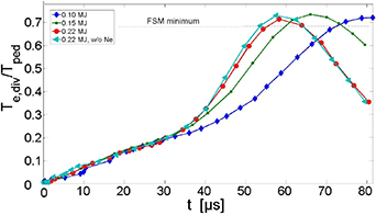
Figure 1. Time evolution of divertor-to-pedestal electron temperature ratios during ELMs at JET obtained with the BIT1 code and the parameters of table 1, for various ELM energies. The peaking values of temperature are also shown in figure 6 (smoothed over 40 μs). The dashed line represents the lower boundary of the free-streaming model (equation (3)).
Download figure:
Standard image High-resolution imageTable 1. BIT1 simulation parameters corresponding to the output shown in figure 1.
| Inter-ELM |
 (eV) (eV) | ne (1019 m−3) |
| Inner divertor | 1.5 | 8.1 |
| Outer divertor | 2.1 | 7.3 |
| OMP | 71 | 1.4 |
| Intra-ELM, run |
 (eV) (eV) | EELM (MJ) |
| 1 | 300 | 0.1 |
| 2 | 500 | 0.15 |
| 3 | 750 | 0.22 |
The type-I ELM characteristics are taken from our previous JET model [11]. In the simulations, the smallest time Ω−1 (electron cyclotron frequency) and space ρe (gyro-radius) scales were resolved. The number of spatial cells was 106. To ensure the simulations are highly accurate, we use a large number of simulation particles per spatial cell: 220–5500. The simulation ended at 80 μs, corresponding to the peaking value of the divertor electron temperature for the 'slowest' ELM (0.1 MJ). The simulations were performed on the Marconi [12] and IFERC [13] super-computers and took ∼107 core hours overall.
The simulation results in figure 1 show that the normalized peak value of the ELM divertor electron temperature is almost independent of the ELM size, just above ⅔ . This is consistent with the collisionless free-streaming model (FSM) [14, 15] predictions which state that a maximum of a third of the electron energy
  , only the component parallel to the magnetic field, can be transferred to ions, as they are naturally pulled behind the fast electrons by the generated parallel electric field, i.e.:

More than ⅓  could be transferred only if the electrons redirect its perpendicular energy into parallel energy, e.g. by collisions. According to our simulations, valid for both JET and COMPASS tokamaks, however, this process is negligible, even with neon injection capable of detaching the inter ELM phase.
3. CAV ELMs on tokamak divertors
The simulation outputs shown in figure 1 are consistent with the observations made on the COMPASS tokamak [9], where the maximum  was shown to be within the collisionless FSM boundaries (equation (3)). These results were obtained thanks to uniquely fast 1 μs resolution measurements of
  as the difference between (not-swept) floating BPP and LP (BPP-LP array). Such a diagnostic is, however, not available on JET and it is therefore necessary to use CAV swept probe measurements during ELMs to infer the
  evolution, as done in [1, 7, 8]. Here, we carefully revisited the data analyzed in [7] in the light of the above-mentioned findings.
3.1. Validation of CAV of ELMs on COMPASS
The CAV technique of ELMs consists of reconstructing IV-characteristics at a much higher sampling rate (the one of the acquisition system) than the applied sweeping frequency (usually below 1 kHz). Assuming that all ELMs are identical events and that their starting time tELM is precisely known, it is possible to associate (current, voltage) couples measured for different ELMs to the same ELM phase. IV-characteristics are then reconstructed at the acquisition system rate and can be analyzed to provide the electron temperature, ion saturation current and floating potential time evolution. Figure 2 illustrates the starting time tELM = 0 detection from Dα measurement with respect to the time traces of the probe current and voltage for two ELMs of COMPASS.

Figure 2. CAV technique first precisely detects tELM = 0 using a spectroscopy signal Dα of many dozens of identical ELMs (here, two are shown), each detected at a random phase of the slow triangular voltage sweep (blue curve). Then, current–voltage characteristics are constructed with respect to the ELM phase tELM, and examples are shown in figures 3 and 5.
Download figure:
Standard image High-resolution imageThe main drawback of the CAV technique is that it relies on the assumption that all events are strictly identical. Furthermore, precise timing of tELM should be obtained to correctly average all ELMs together. Therefore, to validate its usage, we have cross-checked whether the CAV slowly-swept LP technique provides similar values to the ones obtained by the fast (1 µs) BPP-LP array measurements in several COMPASS discharges, where both diagnostics were available. If true, it provides an indication that the technique can also be applied to the JET data.
In figures 3(a) and (b), two IV-characteristic examples obtained from COMPASS data are shown: the first one was obtained before the ELM rise (inter ELM) and shows a very low scatteredness of the points and a subsequent good accuracy of the fit, while the second one was obtained at the ELM peak (maximum temperature) and the data are much more scattered.
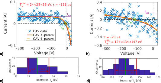
Figure 3. CAV IV-characteristics of the swept probe data (each blue cross corresponds to another ELM) and their fits (red and orange curves), obtained from 162 ELMs collected from six shots (#20471, #20473, #20477, #20485, #20499) with similar parameters measured by the Langmuir probe LPA 36 on the COMPASS divertor. (a) Dα
ELM time tELM = −131 μs (inter ELM). (b) The ELM peak yields the highest  with relatively high scatteredness. (c), (d) Corresponding histograms of the bootstrap distributions of the electron temperatures, with median (green line) and ⅔ confidence interval (red lines) also depicted.
Download figure:
Standard image High-resolution imageAll IV-characteristics were fitted by both three and four parameters. To enable a better estimate of the parameter errors, the bootstrap technique was applied [16]. Each IV-characteristic is fitted a hundred times, each time with the same number of randomly selected points, meaning that some points are randomly excluded or repeated. This yields a spread of all possible parameters, whose confidence interval (containing two thirds of the data) may be asymmetric, which is the main advantage of the bootstrap method and is further used. This is particularly important for temperatures near and above the available voltage span or for scattered data, where often the maximum possible fit temperature is undetermined [16], whilst the minimum is still relatively precise. Figures 3(c) and (d) show the two bootstrap histogram distributions of the electron temperatures corresponding to the IV-characteristics of figures 3(a) and (b). In the following, we chose the median values of these distributions to be the most representative temperature because it avoids uncertainties due to Te above the voltage span threshold.
In figure 4, the entire ELM time evolution obtained from CAV is compared to the same quantities measured at a much higher rate (1 μs resolution) with the BPP-LP array and only then averaged into the red curve. For the three quantities, a very good match is obtained regardless of whether the three (blue curve) or four (black curve) parameters fits are used. Due to the higher degree of freedom in the four-parameter fit (allowing finite sheath resistivity), the resulting Te is much more scattered due to too limited voltage, thus we do not use it further (also for JET). The agreement of Te is satisfactory during ELMs, although in the inter-ELM there is a difference between CAV and BPP-LP measurement of a factor up to two. Such good agreement was found in all the analyzed cases (shot groups), indicating that both techniques provide credible output.

Figure 4. Entire ELM time evolution obtained by fitting CAV IV-characteristics (blue and black points) of the 162 COMPASS ELMs mentioned in figure 3. For comparison, we show the same quantities measured by the BPP-LP array (1 μs resolution, purple dots) and their time-averaged values (red curve).
Download figure:
Standard image High-resolution imageIn addition, the filaments observed from the BPP-LP array measurements (purple points) are averaged out by the CAV, as the ELM filaments are random, ELM after ELM. Therefore, the ELM peak temperature obtained by CAV (∼200 eV) principally underestimates the real peaks observed by the fast BPP-LP measurements reaching 350 eV.
3.2. CAV of JET ELMs
Since the CAV technique provides reasonable results on COMPASS, it was applied to reanalyze the very same JET data shown in [7]. In figure 5(a), a CAV IV-characteristic obtained at the ELM temperature peak is shown, together with the spatio-temporal evolution of the fitted electron temperature for each JET divertor probe in figure 5(b).

Figure 5. (a) CAV IV-characteristic obtained on probe 18 at tELM = 0.5 ms shown for the worst case, i.e. the temperature peak. The fit (red curve) is still distinguishable from the (green dashed) straight line corresponding to unmeasurably high
 ∼ ∞. (b) Spatio-temporal temperature evolution obtained in the same way. These JET data were obtained by collecting 70 ELMs (from 56 to 57 s) of #91112.
Download figure:
Standard image High-resolution imageFirst of all, the data seem to be well fitted, even up to the maximum electron temperature (figure 5(a )). Second, only probes 18 and 20 observe a significant electron temperature rise (figure 5(b )). This is due to the rather large distance between two consecutive probes (∼2 cm) and damaged probe 19. Third, the peak electron temperature is observed to be 110 eV on probe 18, around half of the pedestal value (240 eV), while a much lower value (25 eV) is reported in [7] for the same shot and time window. This discrepancy between the two analyses is not understood. Similar discrepancies were found for all the reanalyzed shots, as will be shown in the next section.
As a final check, figure 6 compares the time-integrated peak energy fluence  ∥
CAV =
∥
CAV =  γJsat
γJsat
 dt (with γ = 7) during an ELM obtained from the CAV data and the ∥
model predictions from equation (9) in [17]. From the entire analyzed database, only few shots were retained as many of them had too few probes working for the whole ELM duration and often too far from the strike point. Their variation is determined mostly by the peak divertor ion fluence Jsat. The relatively good agreement shown in figure 6 is a further indication that the CAV technique provides reasonable results.
dt (with γ = 7) during an ELM obtained from the CAV data and the ∥
model predictions from equation (9) in [17]. From the entire analyzed database, only few shots were retained as many of them had too few probes working for the whole ELM duration and often too far from the strike point. Their variation is determined mostly by the peak divertor ion fluence Jsat. The relatively good agreement shown in figure 6 is a further indication that the CAV technique provides reasonable results.
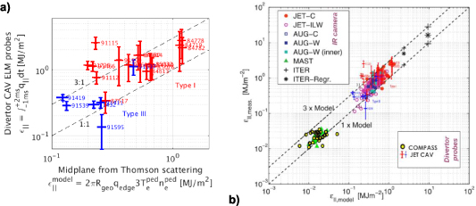
Figure 6. Peak time-integrated divertor CAV ELM parallel heat flux (energy fluence) against the model prediction [17, 18]. (a) Our new data, (b) plot on top of the published data. The confidence intervals (vertical bars) are likely underestimated. Reproduced with permission from [17]. CC BY-NC-ND 4.0.
Download figure:
Standard image High-resolution image4. Reanalyzing the JET ELM temperature ratio divertor over pedestal
On the COMPASS tokamak, we observe a good match between the fast direct and slow CAV measurement of the plasma ELM divertor electron temperature. Even though the peak ELM temperature from the CAV technique provides a slightly lower estimate of the temperature due to averaging out filaments, it still represents a very close match. This further supports the conclusion[9, 19] that the peak ELM temperature on the divertor fits the collisionless free streaming predictions (equation (3)) on COMPASS. This observation is, however, in strong disagreement with what was reported earlier by [1, 7, 8] on JET, where a very low peak ELM temperature was found.
The reanalyzed JET divertor peak ELM Te (smoothed over 40 μs to avoid catching nonphysical peak values), shown in figure 7 and table 2, yields a very different conclusion to what was published earlier. First, the shots for which the ratio  was as low as 2%–10% (all the gray crosses,
  of the analyzed shots) are completely unanalyzable due to a number of limits and problems which may interfere with the maximum ELM peak estimation:
- The discharge conditions must be constant to ensure all the collected ELMs are identical.
- The strike point must be located at a fixed position for sufficiently long periods in order to acquire at least a few dozen ELMs (number of points of the CAV IV characteristic). Often the strike point was moving ∼4 cm (see table 2) which is twice the divertor decay length.
- The voltage must not drop due to over-current.
- The overall voltage range 170 V must be larger than , as discussed in [16]. We estimated the limit of credibility of the ELM peak to be below 170 eV, as demonstrated by the green dashed linear line in figure 5(a
). This limit was overcome for nearly all the shots with higher than 600 eV, meaning that here credible is only the lower estimate of the ELM peak temperatures. Exceptionally for low scattered data, this limit is a bit higher.
- Exact detection of the starting time tELM = 0 of the ELM from the beryllium-II (BeII) spectroscopic line, respectively uncertainty of the mutual time-shifts, must be much shorter than the ELM decay time. On JET data, synchronization with the BeII signal is more tricky than with Dα on COMPASS.


Figure 7. Comparison of the CAV peak ELM temperatures on the JET outer divertor target with the pedestal ones for 74 discharges in [7]. The gray crosses (unanalyzable) and triangles (analyzable) are the previously published results, while the blue circles are the newly achieved values (smoothed over 40 μs to decrease its scatter) and with slightly corrected  values. Around a third of shots see the peak ELM temperature clearly higher than the voltage span 170 eV (i.e. unmeasurably high); their confidence interval is shown according to its drop down to measurable temperatures before-/after-ELM or far outside the strike point. In discharges where significant bootstrap fraction reaches an unmeasurably high Te < ∞, the confidence interval is set to
  . All shown data were individually carefully checked as the most probable peaks, consistent with the space and time neighbors. The exact values are written in table 2. The boundaries of the collisionless free-streaming model are represented as green and violet dashed lines. The temperatures from simulation (see figure 1) are also shown in green (also averaged over 40 μs). R2 is the coefficient of determination, thus quality of the IV-characteristic fits.
Download figure:
Standard image High-resolution image
Second, for 60 reanalyzed shots, we observe much larger peak values of the CAV temperatures than published (the gray triangles vs blue circles).
Third, we have also reanalyzed the pedestal temperatures from Thomson scattering using the approach described in [20]. We found only minor differences with respect to [7] and added vertical error bars in figure 7 and table 2.
Additionally, the BIT1 simulation temperatures are also shown in green in figure 7. They fall around  /
/ ∼ ½, slightly below the collisionless FSM lowest boundary because the data were smoothed over 40 μs to match the smoothing applied to the experimental CAV temperatures. The most credible (high R2) reanalyzed CAV temperatures fall not too far off the simulations results.
5. Discussion
Reanalyzing data from [7], we found that several issues could arise during the analyzing process. For example, many previously analyzed shots are not suitable for performing CAV (e.g. strike point moving) and the ones which are satisfactory yield much higher peak ELM temperatures. We believe that our very careful reanalysis gives a better idea of what the pedestal-to-divertor temperature ratio really is.
However, even for the newly obtained results, most of the temperature ratios are smaller than the lower boundary of the collisionless FSM [14, 15]. This can be understood by recalling that, due to averaging several random filaments together (see figure 4, the pink points vs CAV temperatures), the CAV technique usually underestimates the peak ELM temperature by up to a factor of two on COMPASS. In the JET analysis, since it was really difficult to synchronize the starting time of ELMs, the effect could be even more important. In addition, very often in the analyzed shots, the probe data close to the strikepoint were missing or faulty, thus lowering the peak observable temperature, especially due to poor probe spatial resolution (∼2 cm). Therefore, accounting for all these points, the real peak temperature ratio could well fit the collisionless model boundaries, consistent with what was found on COMPASS [9]. The collisionless assumption is also in good agreement with the BIT1 simulation results (see figure 1).
This result strongly contradicts the conclusion of [1, 7, 8], where one needed to account for collisions to justify the transfer of the perpendicular electron energy (low  ) to the ions, yielding very high ion temperature. Nevertheless, the effect on the sputtering of this correction can only be assessed in future work, including detailed modeling of the plasma–wall interaction. In the case of high Te, even though the ions reaching the divertor are not significantly accelerated by the electrons within the SOL during an ELM crash, a significant portion of the electron energy is transferred from the electrons to the ions inside the plasma sheath anyway (where the magnitude of the potential drop scales with
  ). Moreover, the high electron divertor temperature has significant consequences for tungsten sputtering during the ELMs because the tungsten prompt redeposition can be strongly enhanced by the plasma sheath electric field ∝
  [21, 22]. Therefore, high
  during the ELM will result in lower net tungsten erosion. In addition, the Ti/Te ratio influences the angles at which ions impact on the surface. When Ti ≫ Te, the ions are basically unaffected by the sheath and can hit the surface at grazing angles of incidence. For Ti ∼ Te, the Larmor gyration is strongly distorted in the sheath, resulting in more perpendicular impacts. This effect can influence the magnitude of the sputtering yield. Understanding these phenomena requires the performance of new simulations where higher ELM temperatures are assumed than previously [23].
Acknowledgments
This work has been carried out within the framework of the EUROfusion Consortium, funded by the European Union via the Euratom Research and Training Programme (Grant Agreement No. 101052200—EUROfusion). Views and opinions expressed are, however, those of the author(s) only and do not necessarily reflect those of the European Union or the European Commission. Neither the European Union nor the European Commission can be held responsible for them. We acknowledge Jakub Seidl for help with the bootstrap method, students Ivan Balachenkov and Anna Kharina from EMTRAIC [24] and the Czech Science Foundation, GA22-03950S and GA20-28161S.
: Appendix
Table 2. Overview table comparing the re-analyzed divertor  with the published [7] values. It demonstrates that inter-ELM
  is comparable to the published ELM-peaks, thus much lower than the re-analyzed ELM-peaks reaching up to
  /2. NaN corresponds to an unmeasurable not-a-number value.
| Shot | Time interval (s) | # of ELMs | Te peak distance from strike point S (cm) | Inter-ELM | ELM | Problems | |||
|---|---|---|---|---|---|---|---|---|---|
| Pedestal Thomson Te,max ped (eV) | Divertor probes Te,ELM div (eV) | ||||||||
| [7] | Horacek re-analyzed | [7] | |||||||
| 81878–81883 | 57.9 < t < 58.9 | 6 | Frassinetti | Confidence interval min < mean < max | 30–33 | Few Type-III ELMs detected | |||
| 84580 | 56.4 < t < 57.9 | 43 | 4 | 310 | 312 ± 7 | 20 | 36 < 63 < 144 | 55 | Far from LCFS |
| 84584 | 49 < t < 51.5 | 32 | 3 | 615 | 486 ± 11 | 28 | 72 < NaN < ∞ | 32 | OK |
| 84587 | 50.4 < t < 52 | 36 | 1 | 295 | 399 ± 14 | 49 | 108 < 166 < ∞ | 11 | OK |
| 84589 | 52 < t < 54 | 77 | 1 | 650 | 538 ± 14 | 31 | 117 < 170 < ∞ | 10 | OK |
| 84613 | 53 < t < 55 | 104 | 1–3 | 570 | 505 ± 13 | 33 | 79 < 135 < ∞ | 18 | OK |
| 84614 | 53.1 < t < 53.5 | 18 | 2 | 477 | 472 ± 20 | 30 | 70 < 147 < ∞ | 13 | Too few ELMs |
| 84623 | 46.2 < t < 47.4 | 47 | 0–2 | 798 | 779 ± 33 | 17 | 71 < 127 < ∞ | 28 | OK |
| 84635 | 46.2 < t < 47.8 | 97 | 0 | 641 | 501 ± 19 | 19 | 62 < 99 < 159 | 25 | OK |
| 84678 | 49.8 < t < 51.1 | 52 | 3 | 695 | 566 ± 14 | 18 | 42 < NaN < 165 | 23 | Voltage drop |
| 84682 | 46 < t < 46.7 | 37 | 0–3 | 1165 | 917 ± 36 | 20 | 69 < NaN < ∞ | 32 | OK |
| 84687 | 52 < t < 54 | 133 | 1 | 495 | No HRTS | 34 | 129 < 170 < ∞ | 21 | Voltage drop, otherwise OK |
| 84689 | 49 < t < 51.5 | 39 | 3 | 763 | 578 ± 8 | 20 | 52 < 106 < ∞ | 18 | Voltage drop |
| 84693 | 49 < t < 51.5 | 47 | 3 | 722 | 514 ± 8 | 21 | 41 < NaN < ∞ | 15 | Voltage drop |
| 84694 | 52.5 < t < 54.6 | 60 | 0 | 598 | 516 ± 9 | 17 | 71 < 125 < 193 | 12 | Voltage drop |
| 84700 | 46 < t < 47.5 | 84 | 0–2 | 880 | 688 ± 25 | 17 | 94 < 143 < ∞ | 29 | OK |
| 84718 | 53 < t < 54.5 | 120 | 1 | 547 | 569 ± 10 | 37 | 151 < 201 < ∞ | 23 | OK |
| 84719 | 53.2 < t < 53.8 | 45 | 1–2 | 690 | 651 ± 15 | 28 | 130 < 183 < ∞ | 22 | Voltage drop, otherwise OK |
| 84720 | 62 < t < 63.2 | 69 | 704 | 60 | 91 < 157 < ∞ | 8 | St.Pt. moving by 2 cm | ||
| 84721 | 62 < t < 63.5 | 70 | 690 | 60 | 92 < 155 < ∞ | 7 | St.Pt. moving by 2 cm | ||
| 84722 | 53.2 < t < 53.8 | 33 | 0–2 | 660 | 600 ± 16 | 45 | 132 < 194 < ∞ | 20 | OK |
| 84724 | 52.8 < t < 53.8 | 42 | 0–4 | 833 | ? | 39 | 100 < 195 < ∞ | 21 | OK |
| 84759 | 49 < t < 50 | 37 | 2 | 806 | 15 | Unanalyzable | 11 | Strong voltage drop | |
| 84760 | 50.6 < t < 51.4 | 51 | 2 | 780 | 17 | Unanalyzable | 17 | Strong voltage drop | |
| 84761 | 9 | 2 | 910 | — | Unanalyzable | 13 | Strong voltage drop | ||
| 84772 | 48 | 2 | 715 | 20 | Unanalyzable | 10 | Strong voltage drop | ||
| 84778 | 53 < t < 54.4 | 55 | 2 ± 4 | 960 | 684 ± 12 | 37 | 114 < 209 < ∞ | 26 | MaxTe > 200 credible even with St.Pt. moving |
| 84782 | 53 < t < 54.4 | 56 | 2 | 1053 | 772 ± 15 | 34 | 142 < 204 < ∞ | 25 | OK |
| 84794 | 44.5 < t < 46 | 51 | 0–2 | 1172 | 915 ± 45 | 22 | >200 | 30 | OK |
| 84798 | 44.5 < t < 46 | 35 | 2–10 | 560 | 484 ± 18 | 10 | 71 < 140 < ∞ | 27 | OK |
| 85026 | 51.4 < t < 52.9 | 69 | 3 | 564 | 587 ± 14 | 25 | 197 | 18 | OK |
| 85032 | 51.4 < t < 52.9 | 61 | 0 | 530 | 561 ± 15 | 23 | 74 < NaN < ∞ | 15 | OK |
| 85041 | 52.4 < t < 54 | 31 | 684 | 516 ± 9 | 37 | 81 < 157 < ∞ | 25 | Strike point is far out where only 1 probe (#24) is OK | |
| 85043 | 52.4 < t < 54 | 25 | 580 | 532 ± 14 | 41 | 71 < 139 < ∞ | 17 | ||
| 85046 | 52.4 < t < 54 | 34 | 1 | 520 | 533 ± 11 | 33 | 72 < NaN < ∞ | 24 | |
| 87517 | 55.5 < t < 57 | 106 | 2 | 560 | 446 ± 44 | 25 | 80 < 134 < ∞ | 26 | OK |
| 87587 | 54.2 < t < 55.4 | 77 | 0 | 350 | Uncertain | 17 | 65 < 84 < 103 | 28 | OK |
| 87588 | 60.44 < t < 60.54 | 1 | 550 | Unanalyzable | 41 | Too few ELMs | |||
| 87874 | 59 < t < 61 | 123 | 240 | Unanalyzable | 25 | Saturated voltage, too messy | |||
| 89426 | 52 < t < 54 | 88 | ±5 | 562 | Unanalyzable | 19 | Strike point movement by 5 cm | ||
| 89708 | 52 < t < 53.6 | 53 | 3 | 408 | 397 ± 7 | 83 | 164 < 201 < ∞ | 30 | OK |
| 90405 | 45 < t < 46.5 | 131 | 1 | 355 | 318 ± 13 | 20 | 62 < 108 < 185 | 32 | OK |
| 90406 | 45 < t < 47.5 | 223 | 1 | 412 | 390 ± 14 | 25 | 98 < 136 < ∞ | 37 | OK |
| 90580 | 54 < t < 56 | 90 | 1 | 310 | 291 ± 11 | 36 | 101 < 116 < 135 | 56 | OK |
| 90998 | 59 < t < 61 | 111 | 1 | 158 | 188 ± 5 | 24 | 92 < 116 < 163 | 24 | OK |
| 91112 | 56 < t < 57 | 70 | 0 | 240 | 237 ± 11 | 24 | 79 < 101 < 136 | 25 | OK |
| 91115 | 57 < t < 60 | 140 | 0 | 230 | 217 ± 7 | 35 | 98 < 115 < 151 | 35 | OK |
| 91411 | 49 < t < 51 | 287 | 0 | 200 | 355 ± 23 | 18 | 57 < 65 < 75 | 32 | OK |
| 91419 | 49 < t < 51 | 231 | 0 | 160 | 176 ± 19 | 20 | 63 < 70 < 85 | 28 | OK |
| 91432 | 49 < t < 51 | 348 | 0 | 175 | 295 ± 32 | 17 | 55 < 69 < 132 | 37 | OK |
| 91466 | 57 < t < 58 | 60 | 0 | 329 | 295 ± 11 | 35 | 95 < 115 < 140 | 46 | OK |
| 91539 | 48 < t < 50 | 111 | 0–2 | 150 | 175 ± 12 | 12 | 58 < 68 < 81 | 50 | OK |
| 91595 | 55.4 < t < 55.9 | 56 | 0–2 | 520 | 476 ± 41 | 36 | 86 < 155 < ∞ | 40 | OK |
| 91597 | 55.15 < t < 55.6 | 46 | 0 | 305 | ? | 29 | 118 < 189 < ∞ | 53 | OK |
| 91599 | 56.5 < t < 56.9 | 22 | 0–1 | 505 | 386 ± 19 | 29 | 104 < 197 < ∞ | 53 | OK |
| 91603 | 56 < t < 57 | 53 | 2 | 540 | 455 ± 26 | 39 | 127 < 180 < ∞ | 40 | OK |
| 91605 | 54 < t < 54.5 | 29 | 293 | Unanalyzable | 42 | Saturated voltage | |||
| 91606 | 55 < t < 56 | 29 | 1 | 510 | 29 | 100 < 130 < 250 | 49 | Few ELMs | |
| 91610 | 54.5 < t < 56 | ±4 | 434 | Unanalyzable | 9 | LCFS is oscillating ±4 cm | |||
| 91611 | 54.2 < t < 55 | ±4 | 513 | Unanalyzable | 8 | LCFS is oscillating ±4 cm | |||
| 91725 | 53.2 < t < 54 | 78 | 1 | 210 | 203 ± 10 | 36 | 87 < 125 < 183 | 58 | OK |
| 91962 | 52 < t < 53.4 | 103 | 716 | Unanalyzable | 47 | Only 2 probes near St.Pt. | |||
| 92130 | 48.5 < t < 49.5 | ±4 | 850 | Unanalyzable | 9 | LCFS is oscillating ±4 cm | |||
| 92135 | 48.5 < t < 49.5 | ±4 | 820 | Unanalyzable | 6 | LCFS is oscillating ±4 cm | |||
| 92141 | 48.3 < t < 49.2 | ±3 | 770 | Unanalyzable | 9 | LCFS is oscillating ±3 cm | |||
| 92332 | 52.4 < t < 53.6 | 50 | 4 | 625 | 534 ± 11 | 60 | 164 < 211 < ∞ | 45 | OK |
| 92335 | 52.4 < t < 53.6 | 47 | 4 | 550 | 556 ± 18 | 65 | 169 < NaN < ∞ | 39 | OK |
| 94248 | 48.5 < t < 52 | 395 | 0 | NaN | 421 ± 9 | 50 | 127 < 159 < 190 | OK | |
| 97421 | 48.6 < t < 51.3 | 192 | 0 | NaN | No data | 47 | 126 < NaN < ∞ | OK | |