


Abstract
An analysis workflow has been developed to assess energy deposition and material damage for ITER vertical displacement events (VDEs) and major disruptions (MD). This paper describes the use of this workflow to assess the melt damage to be expected during unmitigated current quench (CQ) phases of VDEs and MDs at different points in the ITER research plan. The plasma scenarios are modeled using the DINA code with variations in plasma current Ip, disruption direction (upwards or downwards), Be impurity density nBe, and diffusion coefficient χ. Magnetic field line tracing using SMITER calculates time-dependent, 3D maps of surface power density q⊥ on the Be-armored first wall panels (FWPs) throughout the CQ. MEMOS-U determines the temperature response, macroscopic melt motion, and final surface topology of each FWP. Effects of Be vapor shielding are included. Scenarios at the baseline combination of Ip and toroidal field (15 MA/5.3 T) show the most extreme melt damage, with the assumed nBe having a strong impact on the disruption duration, peak q⊥ and total energy deposition to the first wall. The worst-cases are upward 15 MA VDEs and MDs at lower values of nBe, with q⊥,max = 307 MW m−2 and maximum erosion losses of ∼2 mm after timespans of ∼400–500 ms. All scenarios at 5 MA avoided melt damage, and only one 7.5 MA scenario yields a notable erosion depth of 0.25 mm. These results imply that disruptions during 5 MA, and some 7.5 MA, operating scenarios will be acceptable during the pre-fusion power operation phases of ITER. Preliminary analysis shows that localized melt damage for the worst-case disruption should have a limited impact on subsequent stationary power handling capability.
Export citation and abstract BibTeX RIS
1. Introduction
Unmitigated thermal and electromagnetic loads from major plasma disruptions (MDs) and vertical displacement events (VDEs) can be potentially very damaging to ITER plasma-facing components (PFCs). This is one of the key drivers for the development of an effective disruption mitigation system (DMS). Operation of ITER will follow a staged approach, beginning with a first plasma phase, two pre-fusion power operation (PFPO) phases and finally the fusion power operation (FPO). Before the PFPO campaigns, the full complement of PFCs, comprising the beryllium (Be) first wall panels (FWPs) and tungsten (W) divertor, will be installed. A detailed ITER research plan (IRP) [1], describes how operation will proceed in order to reach the key ITER mission goals, with the first being the achievement of QDT = 10 operation at the baseline plasma current and toroidal magnetic field of Ip = 15 MA and Bt = 5.3 T. One feature of the IRP is that experiments are performed in a step-ladder approach from PFPO to FPO phases with steadily increasing performance moving through pairs of Ip and Bt such that the baseline equilibrium with safety factor q95 = 3 is consistently used. This yields three main combinations at 1/3, 1/2 and full field and current (5 MA/1.76 T, 7.5 MA/2.65 T and 15 MA/5.3 T). The first non-nuclear phase, PFPO-1, will establish diverted plasma operations with hydrogen (H) or helium (He) plasmas, up to at least 7.5 MA/2.65 T in L-mode (and possibly up to 10 MA), and will attempt H-modes at 5 MA/1.8 T. In PFPO-2 with all the installed additional heating power available, 15 MA/5.3 T L-mode operation and 7.5 MA/2.65 T H-mode operation in H or He will be the main focus. Only in the FPO phase will deuterium (D) and eventually tritium fuel be introduced.
An important question is: when in the staged approach will unmitigated VDEs and MDs become problematic with regard to PFC lifetime? Melting of PFCs will occur during both the thermal quench (TQ) and current quench (CQ) of unmitigated disruptions on ITER at and beyond the maximum values of thermal and magnetic stored energy [2]. The most susceptible components earlier in the research plan will be the Be FWPs. This is because the melting temperature of Be is relatively low (cf W), but also because the conversion of poloidal field magnetic energy to plasma thermal energy in the halo current during the CQ can lead to strong main chamber interactions even at comparatively low Ip. Assessing the magnitude and consequences of these CQ-induced melt events during the unmitigated CQ for different phases of the IRP is the main purpose of this paper.
A workflow has been developed to assess energy deposition and PFC damage for ITER VDEs and MDs. The workflow methodology: 2D magnetic flux profiles from DINA simulations [3] provide input to the SMITER 3D field-line tracing software [4], producing 3D maps of perpendicular surface heat flux q⊥ and magnetic field  on the FWPs. These maps are then used to compute time-dependent melt formation and motion with the MEMOS-U code [5, 6], accounting for heat flux reduction by plasma vapor shielding [7]. The melt-damaged FWP models are subsequently regenerated in SMITER, allowing an assessment of enhanced heat loads from either stationary scenarios or a subsequent VDE/disruption. This paper will analyze a selection of the DINA disruption (VDE and MD) dataset using the described analysis workflow.
2. DINA disruption dataset
The DINA code computes magnetic equilibria and 1D transport for the development of plasma scenarios and the analysis of plasma disruptions [3, 8]. The appendix of [8] gives detailed descriptions of DINA's underlying equations, and a description of the power balance during VDEs and MDs is provided in [9]. These DINA disruption simulations begin with an appropriate stationary equilibrium scenario, and then perturb that equilibrium to initiate either a VDE or MD. In the case of an unmitigated (hot) VDE, a vertical perturbation is applied to the stationary equilibrium and the plasma moves up or down. Once the last closed flux surface (LCFS) makes contact with the 2D wall contour, the TQ is triggered in the code. At the time of the TQ, Be impurities are introduced instantaneously after the prescribed loss of the plasma thermal energy. The code then calculates the evolution of the CQ phase, including halo current dynamics. Simulations of the MDs are similar, except that in this case the TQ is triggered before any plasma motion or FWP contact. Thus, the MDs have time to evolve and radiate away energy during the CQ phase before any contact with the wall.
The latest version of DINA, with updates described in [10], has been used to compile 84 ITER disruption scenarios relevant to PFPO-1 up to FPO. Variations in this disruption database include Ip, Bt, disruption direction (up or down), Be impurity density, cross-field thermal diffusivity coefficients (χ), and disruption type (VDE vs MD). No disruption avoidance or mitigation methods are assumed, such that the maximum CQ time (tCQ) and energy deposition are realized. The most important outputs from DINA are the time-dependent flux maps (Ψ(r, z)), the radial parallel heat flux distribution q∥(r) in the halo region, and the total energy Edep deposited on the first wall (FW). Edep is the total amount of magnetic energy deposited on the FW through conduction along open magnetic field lines (q∥(r)), based on the power balance in DINA in combination with radiative loss terms [9].
As described in section 1, variations in Ip and Bt match the q95 = 3 scenarios envisioned for PFPO: 5 MA/1.8 T, 7.5 MA/2.65 T, and 15 MA/5.3 T. The starting core plasma electron density ne is varied accordingly: 3 ⋅ 1019 m−3 at 5 MA, 5 ⋅ 1019 m−3 at 7.5 MA, and 10 ⋅ 1019 m−3 at 15 MA. For each of these scenarios (for both VDEs and MDs), there are at least two values for the assumed perpendicular transport coefficient χ: 1 m2 s−1 and 4 m2 s−1. The Be impurity concentration, nBe, is assumed uniform at the start of the TQ and varies from 0, 1 ⋅ 1019 m−3, and 3 ⋅ 1019 m−3. This impurity model in DINA is simple. In reality, nBe in the plasma core and edge will vary in time and location as the VDE interacts with the FW. This nBe would be in addition to impurities present in the plasma during stationary operations from sputtering/erosion of the FWPs. A self-consistent model of impurity introduction as the disruption evolves is not currently available in DINA. As discussed in section 3 of [10], the maximum assumed nBe is not unrealistic for a VDE originating from a 15 MA, H-mode burning plasma scenario. For the lower power cases at 5 MA, with a starting ne of 3⋅ 1019 m−3, an introduction of nBe = 3 ⋅ 1019 m−3 would result in a mostly Be plasma (Zeff = 3.4 post-TQ), but such plasmas may not be unreasonable based on observations on JET (figure 8 of [11]) so they are covered here for consistency. Tungsten impurity present prior to the TQ (resulting from erosion of the divertor targets) is neglected due to the low concentrations and its relatively low cooling power.
2.1. Comparison of DINA halo current model with experiments
As discussed in [10], the latest DINA version used to create this database incorporates a number of significant updates. The SMITER and MEMOS-U results in sections 3 and 4 emphasize the influence of the disruption dynamics on surface heat flux q⊥, surface temperature rise, and melt damage. Therefore, it is important to keep in mind the assumptions made in the DINA model, as well as to compare with experimental observations where possible. Of particular importance is the accuracy of the halo current density Jh. Halo current dynamics play a strong role in calculating both electromagnetic and thermal loads [9, 10]. The term halo width, wh, is often used as a way to quantify the spatial distribution of Jh.
A unique first attempt at comparing the DINA halo model to measurements of wh across various tokamaks is given in [10]. In general, extrapolation of wh data to ITER is not straightforward due to experimental differences in machine size and geometry, diagnostic limitations, and varying definitions of wh used in publications. To compensate for these difficulties and limitations, wh is defined as a physical width (in meters) mapped to the outer midplane (OMP) of the quenching plasma, with a cut-off point arbitrarily chosen as the last radial point at which the magnitude of Jh falls below 5% of the maximum. Mapping wh along magnetic-field lines to the midplane eliminates differences in local wall geometry. Additionally, comparing wh as a function of minor radius (a) compensates for large differences in tCQ between devices. Finally, normalizing the values of wh and a to the major radius (R) compensates for variations in machine size. Using this comparison methodology, the wh data reported in [10] has been expanded and is given in figure 1, which includes data from COMPASS [12, 13], JET [14], Alcator C-MOD [15], and ASDEX-Upgrade [16, 17].
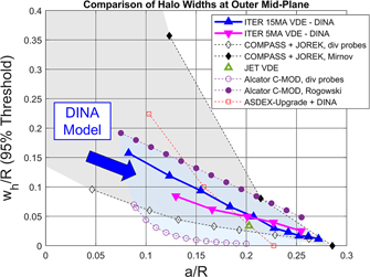
Figure 1. Halo width wh as a function of minor radius, normalized to device major radius. Experimental data is given with dashed lines, with solid markers for upper-bound data and open markers for lower bound data. DINA data for ITER is given by solid points and solid lines. As VDE or MD time increases, minor radius (a) decreases.
Download figure:
Standard image High-resolution imageIn all cases, experimental data is coupled to simulation reconstructions of the CQ poloidal flux maps to estimate minor radius and map Jh deposition locations back to the OMP. Lower and upper bounds have been added for COMPASS (shaded in gray) as well as C-MOD (shaded in blue) using downward VDE experiments. For COMPASS, a lower-bound is calculated from divertor probes (which do not measure the entire extent of wh) [12], while an upper-bound is derived from Mirnov coil data. Both datasets are paired with dedicated JOREK simulations of the downward VDE. For C-MOD, a lower-bound is calculated from a divertor 'rail' probe array [15] averaged across shots 1160707004–1160707007 and 1160707009. A rough upper-bound is estimated based on Rogowski coils for separate, but similar, downward VDEs during shots when the full coil array was present (shots 950214037–950214041). Datasets are paired with a current filament reconstruction tool [15]. Neither dataset from C-MOD was able to measure the entirety of wh by meeting the 5% threshold requirement, but they provide the best possible estimates of wh given the available diagnostics. The ASDEX-Upgrade dataset uses a poloidal array of shunts across the lower divertor and inner-wall heat shields, which does observe the full wh, but with low spatial resolution [16, 17]. Three experimental data points for shot 25000 are paired with DINA simulations (see figure 3 of [17]). The single data point from JET is measured on the upper dump plate by toroidal field pick-up coils and Rogowski coils [14] and paired with an EFIT reconstruction.
The important conclusion is that wh values for ITER CQs modeled with DINA fall within this wide range of experimental data. This builds confidence in the DINA predictions for wh, Jh(r) and q∥(r), which impact the magnitude and distribution of q⊥(r) in time. Still, it should be noted that there is a large uncertainty in the experimental data, particularly at the end of the VDE when a is small (and when q⊥ is usually more severe). Continued effort by the fusion community to cross-compare halo current data across tokamak devices, using a common scaling and a fixed definition of wh, is essential and strongly encouraged for extrapolation to ITER.
3. SMITER heat flux analysis
The next step in the workflow is a 3D heat flux analysis using the SMITER field-line tracing software [4]. SMITER utilizes the time dependent plasma equilibrium Ψ(r, z),  , and Edep from DINA. Magnetic field lines are traced from the 3D target geometries (in this case the Be FWPs and W divertor) to determine areas that are magnetically shadowed by upstream components. By relating the unshadowed field lines to
  , and accounting for the field line intersection angle on the PFC surfaces, maps of q⊥ are generated for any target PFC of interest. To guarantee that the 3D power balance in SMITER matches the 0D power balance in DINA, a scaling factor is applied to q∥(r). This scaling takes into account the 3D, non-uniform power deposition observed in SMITER and also corrects the pitch angle definition of q∥ within DINA to be q∥ along the magnetic field lines. SMITER uses Phalo, the total power within the halo region (calculated based on Edep), as the value for power in the scrape-off layer, PSOL. The code does not dynamically account for power generation in the halo region and instead assumes that the entirety of Phalo is deposited onto the FW. The SMITER FWP geometries are smooth curved surfaces, as in [10, 18], with a triangular mesh resolution of ∼5 mm.
A considerable portion of the DINA disruption database has been evaluated in SMITER, 38 of 84 available cases. The selection covers the worst-case scenarios for ITER and is broad enough to study the importance of Ip/Bt, nBe, χ, and disruption direction for both VDEs and MDs. During the CQ, the upward VDEs/MDs deposit all the conducted energy on the upper FWPs, meaning that FWPs #7, #8, and #9 at the top of the machine will be at the greatest risk of melt damage (see figure 2). The downward VDEs/MDs deposit their energy on both the Be FWPs and on the outer baffle region of the W divertor vertical target (see figure 3). The power balance mentioned above does account for all components. However, the focus of this work is on the Be FWP material response. Work is ongoing at ITER for further evaluation of W melt damage using this analysis workflow.

Figure 2. Example map of q⊥ calculated in SMITER for an entire poloidal sector of Be FWPs. The case is for a 15 MA upward VDE (nBe = 3 ⋅ 1019 m−3, χ = 1 m2 s−1) at the time of max q⊥ (Δt = 200 ms).
Download figure:
Standard image High-resolution image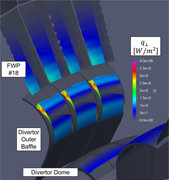
Figure 3. Example map of q⊥ calculated in SMITER for a 15 MA downward VDE (nBe = 1 ⋅ 1019 m−3, χ = 1 m2 s−1) at the time of max q⊥ (Δt = 80 ms). q⊥,max = 150 MW m−2 for FWP #18.
Download figure:
Standard image High-resolution imageFor upward disruptions, the peak heat flux, q⊥,max, usually occurs toward the end of the CQ. This is when the plasma LCFS is smallest, causing the magnetic field lines to intersect at relatively large angles. Edep also generally peaks near the end of the disruption which, when combined with larger field-line angles, further magnifies q⊥,max. For downward cases, the LCFS usually limits on the divertor outer baffle. As the quenching plasma grows smaller and field-line intersection angles increase, the LCFS moves farther away from FWP #18. Since  is an exponentially decreasing distribution (see [10]), this balances out to give a q⊥,max in the middle of tCQ, with q⊥ decreasing as the plasma shrinks and quenches on the divertor outer baffle. Thus, the downward VDEs are always less severe than their corresponding upward cases for the Be FWPs.
In general, the VDE/MD time and heat flux intensity both increase with Ip and Bt. Consider the upward VDE as an example (nBe = 3 ⋅ 1019 m−3, χ = 1 m s−1). At 5 MA/1.8 T, the VDE lasts for ∼75 ms and deposits ∼29 MJ on the FW with q⊥,max ∼ 83 MW m−2. At 7.5 MA/2.65 T, those values increase to ∼120 ms, ∼79 MJ, and q⊥,max ∼ 130 MW m−2. Finally, for 15 MA/5.3 T, the VDE persists for ∼250 ms and deposits ∼420 MJ with q⊥,max ∼ 320 MW m−2. Figure 2 shows the 3D distribution of q⊥ for this high current VDE at the time of q⊥,max.
When comparing VDEs and MDs, the MDs often show a slightly higher energy deposition area, tCQ, and Edep. The value of χ has minimal impact on the CQ dynamics and heat flux when a non-zero nBe is assumed. Scenarios with χ = 1 m2 s−1 give slightly higher values of q⊥, so only these scenarios are considered for the next step in the analysis. Conversely, the assumed nBe has a strong effect. Variation in nBe significantly influences the tCQ, Edep, Phalo, and q⊥,max for all cases. Figure 4 highlights the impact of nBe for upward VDE and MD scenarios. In general, a higher nBe in the halo region leads to a shorter tCQ and smaller magnitudes of total halo current Ihalo. Radiative and ohmic losses are higher, causing less energy from the halo currents to be conducted along magnetic field-lines to the FW. However, a lower total Edep over a shorter time balances out to give increased q⊥. For the previously described 15 MA/5.3 T VDE (nBe = 3 ⋅ 1019 m−3, χ = 1 m2 s−1), lowering nBe to 1 ⋅ 1019 m−3 increases tCQ to ∼400 ms and Edep to ∼590 MJ. The q⊥,max over that longer timespan reduces slightly, to ∼307 MW m−2. The same relationships with nBe are observed for the MD scenarios to a more pronounced degree. For the MDs, the TQ and its associated influx of Be impurities occurs before the plasma makes contact with the FW. The DINA disruption scenarios assuming nBe = 0 give an extremely long tCQ. The same 15 MA, χ = 1 VDE case with nBe = 0 lasts for almost 3 s. With no radiative energy loss, a full ∼940 MJ of conductive energy is calculated for the FW. As a result of the long energy deposition duration, q⊥,max reaches only ∼55 MW m−2. The radiation loss term is a vital component to the DINA power balance (see equation (2) of [9]), and any disruption will introduce Be (and W) impurities during both the TQ and CQ phases. For these reasons, the scenarios for nBe = 0 need not be considered for the next step in the analysis.

Figure 4. Maximum surface heat flux q⊥,max vs. disruption time. VDE data is given by solid lines, with the corresponding MDs given by dashed lines of the same color. Data for the cases of nBe = 0 extend outside of the plot, up to ∼2750 ms and 3300 ms for the VDE and MD, respectively. Δt = 0 represents the point at which Edep becomes >1 MJ.
Download figure:
Standard image High-resolution image4. MEMOS-U melt damage predictions
The MEMOS-U melt dynamics code [5, 6] is used to model the formation and motion of molten Be on the ITER FWPs under unmitigated disruption transients. The code solves the incompressible resistive thermoelectric MHD equations in the magnetostatic limit, along with the convection–diffusion equation for temperature. Material properties for solid and liquid Be are compiled for MEMOS-U with sources listed in [5, 18]. For energy deposition during the CQ phase of a disruption, melt motion is driven by a volumetric  force within the shallow melt layer.
MEMOS-U requires the 3D maps of q⊥ and  vectors from SMITER as input. Ihalo is calculated from DINA at each time step, and then evenly distributed as a density
  across the total wetted area calculated in SMITER. In reality,
  will vary across this wetted area and will depend on the parallel current density
  within the halo region. The directionality of
  is properly implemented to account for the fact that the halo current flows into the FWPs on one side of the LCFS contact point and flows out of the FWPs on the other side. This characteristic of
  leads to different melt-motion directions on either side of the LCFS contact point (see figure 6). For all results presented here, the MEMOS-U rectangular domain resolution is 5 × 5 mm across the FWP surface, to match the SMITER mesh lengths.
It should be emphasized that macroscopic melt motion of Be under disruption CQ transients has been clearly documented on JET [19]. During the first JET ITER-like wall campaigns, a small number of upward going, unmitigated VDEs led to macroscopic motion of Be on the limiter tiles (referred to as 'dump plates') at the top of the main chamber. The melt layers were observed to move poloidally from the high to low field sides. The same directions of Ip and Bt in these JET discharges will be used for ITER. The  flow directions and melt motion directions in this paper match the JET observations, with Be melt on the outboard side of the LCFS flowing in the outboard direction. In fact, MEMOS-U has recently been used to successfully model the observed JET dump plate melt damage [6], building confidence in the results presented for ITER in section 4.2 below.
4.1. Vapor shielding in MEMOS-U
One unique aspect of this work is the incorporation of a vapor shielding model in MEMOS-U. As heat and particle fluxes impact the FWP material surface, individual Be atoms are ejected from the surface via sputtering, evaporation, and/or ablation. Such ejection forms a vapor layer of Be just above that surface. This layer is then ionized and excited via successive heat and particle fluxes, ultimately 'shielding' the underlying surface by reducing the impinging fluxes. The presence of a vapor shield can reduce the surface temperature rise, which can in turn affect the melt formation and the surface modification profile.
The PIXY code uses a particle-in-cell (PIC) model for the plasma, accounting for edge plasma properties and sheath physics up to a solid surface [7]. The motion and interactions of electrons, hydrogen ions, and wall-derived vapor particles are solved in 1D space but with 3D velocity (1d3v). A 1D heat transfer model is coupled to PIXY to estimate the surface temperature, Tsurf, in this case a Be FWP model with 10 mm of Be, 7 mm of copper, and cooling water at 343 K. Dedicated PIXY simulations have been performed for the ITER disruption energy deposition analysis workflow [20]. Parameters from DINA VDE scenarios at 5 MA, 7.5 MA, and 15 MA have been used as input for a range of PIXY simulations, such as ne, Te,  magnitude and average impact angle (see table 1 of [20]). Due to the heavy computational requirements of PIC simulations and long VDE times (hundreds of ms), a simple implementation is chosen. An analytic function for the vapor shielding efficiency ɛVS as a function Tsurf and q⊥ is fitted to the PIXY data for each value of IP. These functions are implemented in MEMOS-U for interpolation. They are given in equations (2) and (3), with coefficients listed in table 1. The PIXY datasets cover Tsurf = 1400–2200 K (the melting point of Be is ∼1560 K) and q⊥ = 50–1000 MW m−2. The fit for equation (3), for the case of IP = 5 MA, uses a limited dataset of q⊥ < 250 MW m−2 to achieve a better fit in regions relevant to 5 MA scenarios.

Table 1. PIXY vapor shielding fit coefficients.
| Coefficients | 15 MA | 7.5 MA | Coefficients | 5 MA |
|---|---|---|---|---|
| P00 | 0.451 441 | 0.439 837 | a1 | 0.019 060 |
| P10 | 0.233 913 | 0.299 574 | a2 | 0.373 080 |
| P01 | 0.086 875 | 0.088 530 | a3 | 1850 |
| P20 | −0.071 734 | −0.055 520 | a4 | 0.223 483 |
| P11 | −0.038 549 | −0.046 258 | a5 | 0.000 00489 |
| P02 | −0.005 256 | 0.001 320 | a6 | −0.001 263 |
| P30 | −0.024 159 | −0.037 139 | ||
| P21 | −0.003 870 | −0.000 907 | ||
| P12 | −0.000 415 | −0.004 650 | ||
| P40 | 0.008 948 | 0.007 033 | ||
| P31 | 0.005 836 | 0.011 116 | ||
| P22 | 0.004 341 | 0.002 296 | ||
| R2 | 0.9915 | 0.9751 | 0.9758 |
At each time point in the MEMOS-U simulations, a reduction in the SMITER q⊥ value is performed at each mesh point based on ɛVS, when vapor shielding is turned 'on'. This implementation scheme is valid so long as the MEMOS-U time steps are much longer than the equilibration time of the vapor shield. PIXY simulations establish the vapor shield on the order of tens of μs, and the MEMOS-U results in section 4.2 use a temporal resolution on the order of ms. The other inherent assumption is that the vapor shield calculated above each ∼5 mm mesh grid stays in place over the MEMOS-U time step. 2D spatial motion of the Be vapor cloud (parallel to the FWP surfaces) cannot be calculated in PIXY and would require a different modeling scheme such as the TOKES code [21]. For the worst-case VDE/MD scenarios from section 3, ɛvs values up to 0.5 are observed by the end of the disruption. From equation (1), ɛVS = 1 implies a full reduction of q⊥ to 0.
4.2. MEMOS-U results
Any variation in the time or total energy deposition will strongly influence melt occurrence and dynamics. The severity of melt damage heavily depends on when during the disruption process the Be surface reaches its melt temperature. Any additional, sufficiently high heat flux can cause the melt layer to increase in depth. Volumetric  forces within that melt layer will then drive macroscopic lateral motion of the melt. Removal of the upper layers of molten Be in areas of continued energy deposition will lead to enhanced heat conduction and melt generation [6]. The resulting melt damage takes the form of excavated pits, where a thickness of Be has been displaced outside the melt pool and resolidified. Thus, the timing of when Tsurf exceeds the melt threshold matters greatly with respect to the VDE/MD duration. More severe melt damage will occur for cases that reach the melt threshold early-on in the disruption.
MEMOS-U simulations have been completed for 16 of the 38 SMITER cases analyzed in the DINA database, with an emphasis on cases with nBe = 1 ⋅ 1019 m−3. Simulation time was extended past the disruption duration long enough (∼100–200 ms) for the 3D melt deformations to stop moving and resolidify. Figures 5(a) and (b) summarize the MEMOS-U analysis efforts, which were conducted for multiple FWPs (#7–9 and #18), with and without the vapor shielding model discussed in section 4.1. Time-dependent values for Jh for these select cases range from 5 ⋅ 103–5 ⋅ 104 A m−2 for the 15 MA cases, 3 ⋅ 103–3 ⋅ 104 A m−2 for 7.5 MA, and 3 ⋅ 103–2 ⋅ 104 A m−2 for the 5 MA cases. The downward cases often exhibit a higher magnitude of Jh than their upward, longer-lasting counterparts.
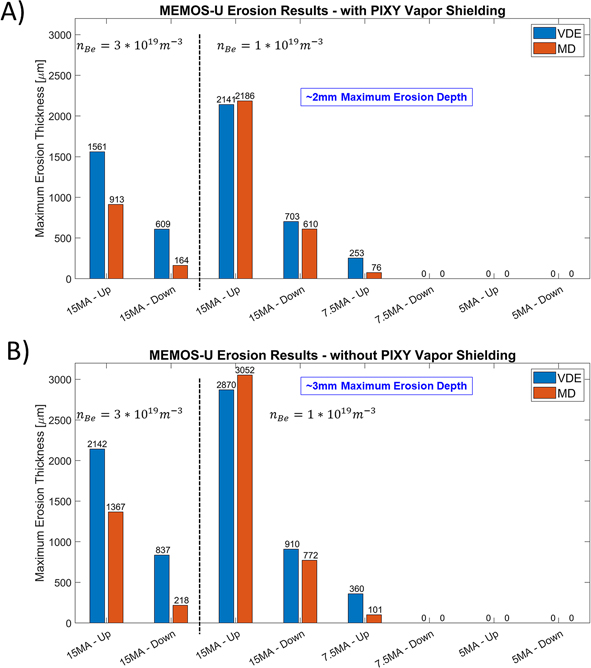
Figure 5. MEMOS-U results for maximum erosion thickness, with (A) including the effects of vapor shielding and (B) not including vapor shielding. The VDE for each scenario is shown by the left, blue bar, and the corresponding MD is shown by the right, red bar. Cases with nBe = 3 ⋅ 1019 m−3 and 1 ⋅ 1019 m−3 are shown to the left and right, respectively, of the vertical dashed line. The maximum erosion thickness occurs on FWP #8 for all upward cases and on FWP #18 for all downward cases.
Download figure:
Standard image High-resolution imageThe damage metric used here is the maximum depth of material loss across the entire FWP surface. For all upward cases, the greatest erosion depth is found on FWP #8. For all downward events, melt damage occurs only on FWP #18. The first key observation from figure 5 is that no melt damage is found for all 5 MA cases (independently of nBe). This was also true for the cases reported in [10]. At 7.5 MA, only the upward VDE with nBe = 1 ⋅ 1019 m−3 shows any melt damage. This is encouraging in showing that the very extensive DMS commissioning planned in the IRP in PFPO-1 can be conducted up to Ip at the 5 MA level without fear of significant damage to the FW. It also demonstrates that for the H-mode operation at 7.5 MA planned in PFPO-2, the DMS will need to achieve a high degree of reliability for CQ mitigation.
Substantial melt damage is observed for all 15 MA VDE and MD cases. At higher nBe (3 ⋅ 1019 m−3), the VDE scenarios are more damaging than the MDs. The higher impurity densities allow for more plasma energy to radiate away at the start of the CQ, before the MD can contact the FW and begin depositing conductive energy. At lower nBe (1 ⋅ 1019 m−3), the MD-induced melt damage is similar to the VDE cases. As stated in section 3, the MD deposits more energy to the FW than VDE, but over a longer tCQ and with slightly lower q⊥,max. In MEMOS-U, the net result is that the MD leads to a similar maximum erosion depth to the corresponding VDE. For the upward 15 MA case, the melt volume displacement is ∼70% higher for the MD than for the VDE due to the increased FWP wetted area. Based solely on the erosion depth, the worst-case scenarios for ITER are the upward 15 MA disruptions with nBe = 1 ⋅ 1019 m−3 and χ = 1 m2 s−1. With vapor shielding included, both the VDE and MD result in maximum erosion depths of ∼2 mm for a single event. This is ∼30% lower than would be the case if shielding was not accounted for (∼3 mm). For the ensemble of VDEs and MDs with melt damage, the inclusion of vapor shielding reduced the erosion thickness by 20%–40%.
Figure 6 shows the 3D distribution of the surface melt displacement across FWPs #7–9 after the worst-case 15 MA VDE and MD with vapor shielding included. Negative values (in blue) represent erosion loss where material is excavated from the original surface. Positive values (in yellow and red) represent build-up of molten Be due to poloidal displacement. The yellow arrows denote the general direction of melt flow. As discussed previously, the  force direction changes depending on whether the halo current is flowing into or out of the FWP wetted area. An important observation in figure 6 is the areal extent of melt damage. Molten Be travels on the order of tens of cm in these simulations, in some cases running off the FWP edges and outside the computational domain. This is analogous to the 'Be waterfall' observed in [19] on JET and modeled in [6]. More importantly for ITER, the Be FWPs are not smooth as in the SMITER models but are castellated. Such extensive Be motion will lead to gap-bridging within the castellated fingers of the damaged panels, as also observed on JET.
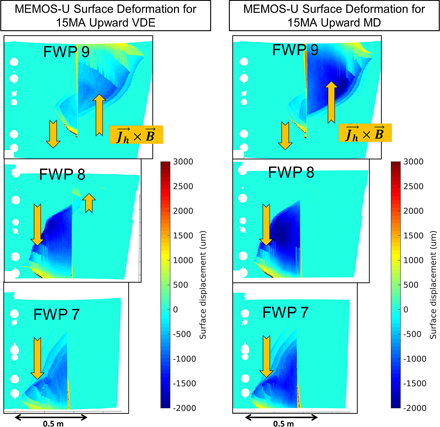
Figure 6. 3D maps of surface deformation on upper FWPs for the worst-case 15 MA upward VDE (left) and MD (right), including the effects of vapor shielding. Yellow arrows indicate the  direction for a given melt area. Toroidal lengths for half of FWPs 7, 8, and 9 are 0.726 m, 0.880 m, and 0.997 m, respectively. Poloidal lengths for FWPs 7, 8, and 9 are approximately 0.80 m, 0.76 m, and 0.83 m, respectively.
Download figure:
Standard image High-resolution imageFigure 7 compiles the time dependence of the maximum Tsurf found on the FWPs for the upward going CQ scenarios in figure 5(a) (which give the worst-case melting). The 5 MA VDE and MD cases stay well below the melt threshold, reaching ∼1230 K and 1050 K, respectively. At 7.5 MA, the VDE and MD cases each last for ∼200 ms, with the melt threshold exceeded only at the end of the CQ. This minimizes the melt and motion that can occur before the surface cools and resolidifies. The 15 MA upward cases achieve a maximum temperature of ∼2300 K over hundreds of ms. The sustained deposition of q⊥ and  at such high Tsurf is what facilitates melt erosion on the order of ∼mm. Interpolating in figure 7 indicates that values of Ip up to ∼7 MA may be tolerable with respect to FWP CQ-induced melt damage, though there is uncertainty here in the absolute values of the halo current densities. Note, assumptions involved in the implementation scheme described in section 4.1, as well as the extrapolation of ɛVS in equation (2) to temperatures above the PIXY dataset might limit the accuracy of high surface temperature values calculated in MEMOS-U. However, since the total absorbed energy is not very sensitive to the shielding details (due to the exponential dependence of evaporation rate on surface temperature) [24, 25], the predictions of melt production (and thereby the results in figures 5 and 6) are robust [5].
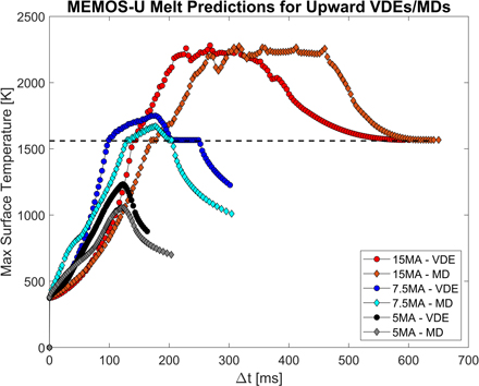
Figure 7. Maximum surface temperature vs. time for upward VDEs (with circular markers) and MDs (with diamond markers). nBe = 1 ⋅ 1019 m−3 and χ = 1 m2 s−1 for all cases (vapor shielding included). The black dashed line marks the melt temperature for Be at 1560 K. MEMOS-U simulation times are longer than the VDE/MD time to allow for re-solidification of melt damage.
Download figure:
Standard image High-resolution imageFor completeness, figure 8 shows the 3D distribution of the surface displacement across FWP #18 for the worst-case downward VDE (Ip = 15 MA, nBe = 1 ⋅ 1019 m−3 and χ = 1 m2 s−1). Figure 9 gives the time dependence of the maximum Tsurf for the downward going scenarios in figure 5(a). As covered in section 3, the downward cases are always less severe than their upward counterparts due to the lower deposited energies and shorter durations.
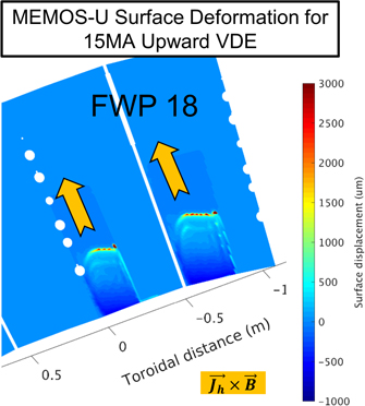
Figure 8. 3D map of surface deformation on FWP 18 for the worst-case 15 MA downward VDE, including vapor shielding. Yellow arrows indicate the  direction for a given melt area. Only half of FWP 18 is simulated.
Download figure:
Standard image High-resolution image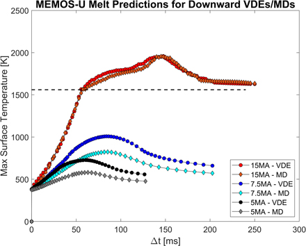
Figure 9. Maximum surface temperature vs time for downward VDEs (with circular markers) and MDs (with diamond markers). nBe = 1 ⋅ 1019 m−3 and χ = 1 m2 s−1 for all cases (vapor shielding included). The black dashed line marks the melt temperature for Be at 1560 K. MEMOS-U simulation times are longer than the VDE/MD time to allow for re-solidification of melt damage.
Download figure:
Standard image High-resolution imageIn fact, melting is only predicted for 15 MA scenarios, with the worst-case resulting in a 0.6 mm erosion depth (with vapor shielding). All others maintain a surface temperature well below the melt threshold.
4.3. SMITER analysis of damaged FWPs
How will melt damage from the worst-case VDEs/MDs impact further stationary operations on ITER? To provide at least a partial answer this question, field-line tracing for the expected stationary plasma scenarios can be performed on the melt-damaged FWP models. Here the worst-case upward VDE from figure 5(a) is analyzed as an example (15 MA, nBe = 1 ⋅ 1019 m−3,  . New FWP meshes are constructed in SMITER for FWPs #7–9, maintaining a ∼5 mm mesh resolution. Each node of the SMITER mesh is displaced along the local surface normal vector, so that the direction of displacement changes with the (pre-damaged) FWP curvature. Each node is displaced using an area-weighted average of the MEMOS-U surface displacement data for every mesh connected to that node. It should be emphasized that SMITER assumes an optical approximation for the particle loads (ions and electrons) along the magnetic field lines. The effect of ion orbits on energy deposition will not be accounted for, even if the FWP surface damage is on the order of the ion gyroradius. These orbital effects will matter most for intra-ELM heat loads, while an optical approximation is likely reasonable for the inter-ELM loads. There should be no issue for the energy component carried by electrons.
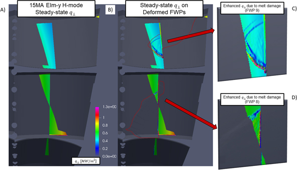
Figure 10(a) depicts the stationary q⊥ distribution for a typical 15 MA, ELM-y H-mode flattop for ITER on undamaged FWPs #7–9 analyzed in [22, 23]. Heat loads include a stationary (inter-ELM) component and an averaged component for mitigated ELMs. For this baseline scenario (the ΔOMP = 0 cm scenario in [22], which has a distance from the first separatrix to the main wall of 17 cm and a distance between the first and second separatrix of 9 cm both at the OMP), heat loads on the upper panels originate from field-lines at and beyond the secondary separatrix. Relatively low values of q⊥,max = 0.65 MW m−2, 1.3 MW m−2, and 0.5 MW m−2 are respectively found on FWPs 7, 8, and 9. The presence of excavated pits and melt build-up will change the local field-line impact angle, and thereby change q⊥, in any areas where the CQ-induced melt damage overlaps with the stationary heat loads. Figure 10(b) shows the resulting stationary q⊥ analysis using damaged mesh models for FWPs #7–9. The melt damage area from figure 6 (left) is highlighted via the dashed red lines, showing that the areas of deepest melt damage do not overlap much with the stationary wetted areas. Although most of the disruption-damaged areas remain shadowed during stationary loading, there are some localized hot spots of increased q⊥ on FWP #8 and #9. On FWP #8, the excavated melt zone leads to a q⊥,max of 1.6 MW m−2 along the apex of curvature. On FWP #9, the presence of melt build-up outside the melt pool leads to a ridge of q⊥,max = ∼2–4 MW m−2. This region is highlighted in figure 10(c). There is no impact on q⊥,max for FWP #7. Similar enhanced q⊥ values are also observed for the worst-case upward MD. Since FWPs #7–9 are 'enhanced heat flux' panels, designed for peak stationary loads of 4.7 MW m−2 [26, 27], all of the 'melt damage enhanced' q⊥ profiles examined here stay below that threshold.
Figure 10. 3D maps of q⊥ for a 15 MA ELM-y stationary H-mode scenario for (A) undamaged FWPs (#7–9) and (B) melt-damaged FWPs for the worst-case 15 MA upward VDE (15 MA, nBe = 1 ⋅ 1019 m−3, χ = 1 m2 s−1). The location of melt damage on FWPs #8 and #9 are indicated by the red dashed area in (B). (C) and (D) give a magnified view of areas on FWPs #9 and #8, respectively, where melt damaged geometries affect the q⊥ distribution.
Download figure:
Standard image High-resolution image
5. Conclusions
Energy deposition and melt damage analysis has been performed for the CQ phase of a wide range of ITER unmitigated VDEs and MDs. These scenarios were simulated with the DINA code and cover pairs of plasma current and toroidal field appropriate to the development of discharges at q95 = 3, which will be pursued within the IRP. The CQ time, total energy deposition and peak heat fluxes on the main chamber beryllium FWPs increase substantially with increasing Ip. The 15 MA/5.3 T disruptions show the most extreme melt damage. For a given Ip, the DINA simulations together with SMITER field-line tracing indicate that the assumed nBe, injected at the start of the CQ plays a major role in the disruption dynamics. Time-dependent MEMOS-U simulations, including vapor shielding, are necessary to determine whether or not each disruption can induce macroscopic melt damage. An important conclusion is the identification of a clear operating window with Ip ≲ 7 MA in which PFC melting may be avoided even without disruption CQ mitigation. This corresponds to the majority of the L-mode operation range currently foreseen in the first ITER non-active operation campaign. In contrast, by the time attempts are made to achieve 15 MA L-mode plasmas in the second non-active phase and burning plasmas in FPO, the ITER DMS must reach extremely high levels of robustness and reliability. ITER must avoid extensive melt-induced erosion and castellation bridging of components due to large scale melt motion driven by halo-current induced forces on the melt layers. Such melt motion on Be surfaces has already been seen experimentally during unmitigated VDEs on the JET tokamak, at much lower CQ durations and magnetic stored energies. Although the predicted final FW melt erosion profiles in localized areas are rather severe, analysis shows that there should be limited impact on subsequent stationary power handling capability, largely because the predicted damage areas do not overlap strongly with the expected regions of power deposition during normal plasma operation.
Acknowledgments
ITER is the Nuclear Facility INB No. 174. This publication is provided for scientific purposes only. Its contents should not be considered as commitments from the ITER Organization as a nuclear operator in the frame of the licensing process. The views and opinions expressed herein do not necessarily reflect those of the ITER Organization. The work of EM was supported by MEYS project 8D15001 and LM2018117. SR would like to acknowledge the financial support of the Swedish Research Council under Grant No. 2018-05273.