Semi-supervised deep networks for plasma state identification

Data used in this paper were extracted from the database of the COMPASS tokamak that was operated by the Institute of Plasma Physics under the Czech Academy of Sciences between 2006–2021 [8]. COMPASS was a mid-size (R₀ = 0.56 m, a = 0.2 m) tokamak with a toroidal magnetic field in the range B_T = 0.8–2.1 T, plasma current up to 400 kA, auxiliary heating by NBI $P_{NBI} \lt$ 1.5 MW, capable of achieving both Ohmic and NBI-assisted H-modes.

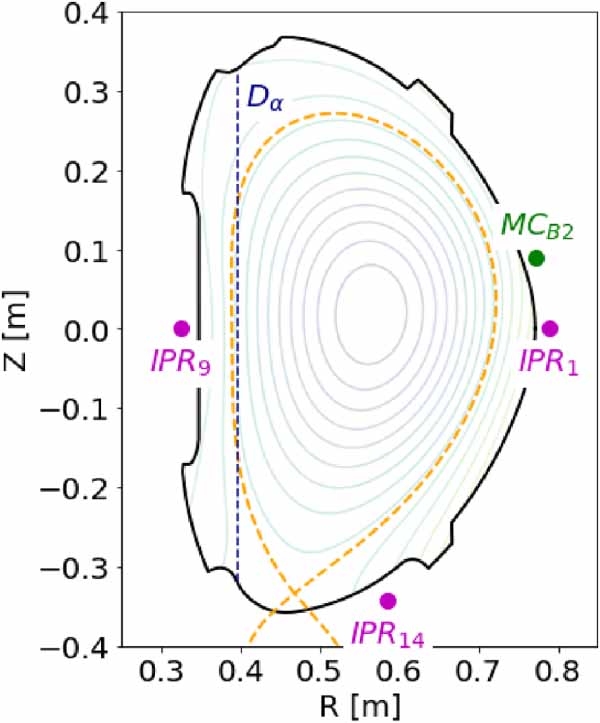
The automatic data collection system of the COMPASS records tens of diagnostic signals for each discharge. However, not all of them are available for all discharges and only a few are known to contain information relevant to the plasma mode classification. Based on expert knowledge of the operators of the COMPASS tokamak, we have selected the five signals as the input features at a given time step: D_α , IPR₁₄, IPR₁, IPR₉ and MC$_{B2}$, summarized in table 1. The location of sensors measuring these data is displayed in figure 2, detailed description of each feature follows.

Zoom In Zoom Out Reset image size

Table 1. List of the signals from the COMPASS tokamak used in detection of the plasma mode.

Abbr.	Description	Sensor
Dα	Radiation of deuterium	Photomultiplier
IPR1	Outer magnetic field	Internal partial Rogowski coil no. 1
IPR9	Inner magnetic field	Internal partial Rogowski coil no. 9
IPR14	Lower part of magnetic field	Internal partial Rogowski coil no. 14
MC$_{B2}$	Outer magnetic field (toridally shifted)	Mirnov coil B theta 02

The D_α signal represents measurement of radiation of the Balmer-alpha line of deuterium (656.1 nm) along vertical chord as illustrated in figure 2 [8]. The amplitude of D_α is strongly correlated with the rate of particle loss from the plasma column. Therefore it is ideal for recognition of plasma states (figure 1) [6].

Internal partial Rogowski (IPR) coils measure the poloidal component of the magnetic field at different poloidal positions around the plasma. In total, the COMPASS tokamak is equipped with more than a hundred magnetic coils surrounding the vessel. From all those signals, we selected only three that are used by the operators for manual mode detection. The sensors are selected to surround the lower part of the plasma, see figure 2. Specifically, IPR₁₄ measures the magnetic field at the lower part of the vessel, while IPR₁ and IPR₉ focus on the outer and inner side, respectively. The IPR₁₄ signal was selected specifically because it is sensitive to the presence of the geodesic acoustic mode, whose presence/absence can be a strong indicator of the plasma regimes [9]. The last signal, Mirnov Coil B theta 02 (MC$_{B2}$), measures a poloidal magnetic field, similarly to IPR, but its toroidal location is shifted from IPR₁ by 155 degrees.

The dataset created for the numerical experiments consists of labeled (L/H/ELM$_{leading}$/ELM$_{trailing}$) and unlabeled discharges. The database of COMPASS contains about 20 000 discharges, but only a few of them have a presence of the H-mode and ELMs fully labeled and revised by researchers.

Therefore, 31 most complete and consistently labeled discharges were chosen for the labeled dataset ($\mathbb{X}_l$) and another 20 unlabeled discharges were randomly selected to form an unlabeled dataset ($\mathbb{X}_u$). The discharges contain a mix of Ohmic and NBI-assisted discharges and ELMing as well as ELM-free H-modes. The total duration of the plasma covered by the dataset is 7303 ms, out of which 4361 ms is labeled as L-mode, 1928 ms as H-mode, 217 ms as ELM-leading edge, and 797 ms ELM-trailing edge (1164 ELM events in total).

In this section, we describe the preprocessing steps that are applied to the raw measured data, independently of the model that is used for prediction. All operations that are specific to the network architecture will be described later in the corresponding sections.

All used signals are recorded with a sampling frequency of 2 MHz. However, the information contained at frequencies above 200 kHz is redundant, so the signals have been downsampled in time by a factor of 10, corresponding to a sampling time 5 µs.

The next step of the preprocessing is scaling. Scaling is needed mainly due to different signals scales and because it allows models to train more effectively. All available data (labeled and unlabeled) were scaled together using the RobustScaler [10]:

$$\begin{equation} \hat{x}_i = \frac{x_i - Q_2(\boldsymbol{x})}{Q_3(\boldsymbol{x})-Q_1(\boldsymbol{x})}, \end{equation} \tag{ 1 }$$

which uses the median $Q_2(\boldsymbol{x})$ and interquartile range ($Q_3(\boldsymbol{x})-Q_1(\boldsymbol{x})$) instead of the common mean and standard deviation. That makes the scaling robust against outliers and abnormally big ELMs that are present in the data.

To exploit the potential of model architectures for sequence modeling (like RNN, CNN, etc), we need to construct overlapping sequences with an assigned label from the individual signals recorded in each time step. However, this requires the decision on the optimal length of the sequences. We have performed a simple feature selection procedure to explore the relevance of the time delayed values of the signals using various classical methods (ANOVA, Mutual information, etc). None of the selected feature sets contained values delayed more than 800 µs. Hence, the downsampled discharges were sliced into fixed-length sequences of length 800 µs. Each sequence contains 160 elements (data vectors from 160 time steps) and the sequences are generated with a stride of 10 (50 µs), i.e. two successive sequences share 150 elements.

Since labels are available for each time step, we need to choose which label to assign for each sequence. We choose to associate each sequence with the label of a sample that appears p µs before the end of the sequence. The p is called label delay and treated as a parameter, see figure 3. For real-time application the lower delay the better:

$$\begin{equation} (\mathbb{X}, \boldsymbol{y})_{p} = \{(x_{n}, x_{n + 1}, \ldots, x_{n + 159}), y_{n+160-p}\}_{n = 0}^{N}. \end{equation} \tag{ 2 }$$

Zoom In Zoom Out Reset image size

Processing of all the included discharges results in a dataset consisting of 128 000 labeled (N_l ) and 97 400 unlabeled (N_u ) sequences, i.e.:

$$\begin{align*} \mathbb{X}_l & = (\mathbb{X}, \mathbb{Y}) = \{\boldsymbol{x}^n, \boldsymbol{y}^n \}_{n = 0}^{N_l}\\ \mathbb{X}_u & = \{\boldsymbol{x}^n\}_{n = 0}^{N_u}, \end{align*}$$

where $\boldsymbol{x}^n \in \mathbb{R}^{5\times 160}$ and $\boldsymbol{y}^n \in \big\{\boldsymbol{y}\in \{0,1\}^4: \sum_{i = 1}^4 y_i = 1~\big\}$ is the one-hot encoded class label.

In order to properly test the performance of the models, we divided the discharges with labels into 20 discharges used for training and 11 discharges used for testing. These discharges were split into sequences and the sequences from the training discharges were divided randomly into the training set (80% of the sequences) and validation set (20% of the sequences). All sequences from the testing discharges form the testing set.

Neural networks (NN) are widely used across various domains, such as image classification, object detection, or natural language processing. However, each domain prefers different types of networks as well as architectures. Recurrent and convolutional neural networks (RNNs and CRNNs) are part of most of the state-of-the-art (SOTA) approaches dealing with sequence modeling.

3.1.1. Recurrent neural networks.

3.1.2. Convolutional neural networks.

3.1.3. Convolutional recurrent networks.

Convolutional recurrent networks (CRNN) are a combination of CRNN and RNNs that should take advantage of both approaches. Convolution layers are typically used for feature extraction from the raw data and then processed with recurrent layers. This type of network was already previously used for plasma classification [6].

The distinction between the above-mentioned architectures is primarily in the way how they process subsequent records in the sequence, as illustrated graphically in figure 4. The RNN assumes a transition model between every time step of the sequence (horizontal arrows between green dots). The convolutional network processes a chunk of the sequence by a convolution filter (denoted by colored triangles). The CRNNs combine those two principles, by modeling a transition model between the results of the convolution filters.

Zoom In Zoom Out Reset image size

3.1.4. Other architectures.

Semi-supervised learning (SSL) is a set of machine learning techniques that use a small amount of labeled data combined with a large number of unlabeled data in order to train or strengthen typically data-demanding models. SSL can also reduce overfitting and help models generalize. One of the methods that allow the exploitation of these attributes is the semi-supervised variational autoencoder (VAE) [16].

3.2.1. Variational autoencoder.

The VAE [17] is a generative model capable of discovering probabilistic distribution $p_{\theta}(\boldsymbol{x})$, which generates data $\mathbb{X} = \{\boldsymbol{x}^n\}_{n = 1}^N$. The key assumption of the model is that the data x is generated by some underlying process, represented by a latent variable z . In principle, the model approximates $p_{\theta}(\boldsymbol{x})$, which is analytically intractable, by introducing the probability distribution of the generating process, $p_{\theta}(\boldsymbol{x}|\boldsymbol{z})$. θ denotes parameters of the distribution. Those are connected through the relation:

$$\begin{equation} p_{\theta}(\boldsymbol{x}) = \int_{\mathcal{Z}} p_{\theta}(\boldsymbol{x}|\boldsymbol{z}) p(\boldsymbol{z}) d\boldsymbol{z}, \end{equation} \tag{ 3 }$$

where $p(\boldsymbol{z})$ is the prior distribution of the latent variable. To enable end-to-end training of the model, the generating distribution is accompanied by an encoding distribution $q_{\phi}(\boldsymbol{z}|\boldsymbol{x})$. That produces such samples z that are most likely to lead to the generation of samples x with a high probability under $p_{\theta}(\boldsymbol{x}|\boldsymbol{z})$, see figure 5.

Zoom In Zoom Out Reset image size

The encoding and generating distribution are usually modeled by Gaussian distributions, with mean and variance being an output of NNs, called the encoder and decoder, respectively. These are optimized simultaneously, using variational inference, in order to maximize (variational) lower bound on the log-likelihood $\log p(\mathbb{X})\geqslant\mathcal{L}(\mathbb{X})$, with:

$$\begin{align} \mathcal{L}(\mathbb{X}) & = \sum_{\mathbb{X}} \mathcal{L}(\boldsymbol{x}) \nonumber\\ & = \sum_{\mathbb{X}} \mathbb{E}_{q_{\phi}(\boldsymbol{z}|\boldsymbol{x})}\Big[ \log p_{\theta}(\boldsymbol{x}|\boldsymbol{z}) \Big] - KL\Big(q_{\phi}(\boldsymbol{z}|\boldsymbol{x})||p(\boldsymbol{z})\Big), \end{align} \tag{ 4 }$$

where the first term on the right-hand side is the expected log-likelihood (negative reconstruction error) and the second term is the KL-divergence between the prior and posterior distributions of z , that regularizes parameters of encoder and forcing $q_{\phi}(\boldsymbol{z}|\boldsymbol{x})$ and $p(\boldsymbol{z})$ to be close to each other.

3.2.2. Semi-supervised VAE.

Standard VAE can be freely extended to a more advanced form, such as the conditional VAE [16], where data are being generated not only by continuous latent variable z but also by discrete latent variable y , that are usually known. The semi-supervised VAE (SSVAE) [18] is special version of conditional VAE, where discrete variables y , e.g. labels, are known only for a fraction of the dataset and thus the encoder needs to approximate a joint posterior distribution $p_{\theta}(\boldsymbol{y}, \boldsymbol{z}|\boldsymbol{x})$ instead of previous $p_{\theta}(\boldsymbol{z}|\boldsymbol{x})$. This extension well matches the need of the studied application.

Assume that z is conditioned by x and y and that the variable y depends only on x , then both distributions can be modeled by separate encoders:

$$\begin{equation} q_{\phi}(\boldsymbol{z}, \boldsymbol{y} | \boldsymbol{x}) = \frac{q_{\phi}(\boldsymbol{z}, \boldsymbol{y}, \boldsymbol{x})}{q_{\phi}(\boldsymbol{x})} \cdot \frac{q_{\phi}(\boldsymbol{x},\boldsymbol{y})}{q_{\phi}(\boldsymbol{x},\boldsymbol{y})} = q_{\phi}(\boldsymbol{z}|\boldsymbol{x},\boldsymbol{y}) \cdot q_{\phi}(\boldsymbol{y}|\boldsymbol{x}), \end{equation} \tag{ 5 }$$

where the approximate posterior distribution of z and y is assumed to be Multivariate Normal and Categorical, respectively,

$$\begin{align} q_{\phi}(\boldsymbol{z}| \boldsymbol{x}, \boldsymbol{y}) & = \mathcal{N}\big(\boldsymbol{~\mu}_{\phi}(\boldsymbol{x},\boldsymbol{y}), \text{diag}(\boldsymbol{\sigma}^2_{\phi}(\boldsymbol{x},\boldsymbol{y}))\big) \end{align} \tag{ 6 }$$

$$\begin{align} q_{\phi}(\boldsymbol{y}|\boldsymbol{x}) & = \text{Cat}(\boldsymbol{\pi}_{\phi}(\boldsymbol{x})). \end{align} \tag{ 7 }$$

Vector functions $\boldsymbol{~\mu}_{\phi}(\boldsymbol{x},\boldsymbol{y})$, $\boldsymbol{\sigma}_{\phi}(\boldsymbol{x},\boldsymbol{y})$ and $\boldsymbol{\pi}_{\phi}(\boldsymbol{x})$ are then represented by NNs. Illustration of such model is shown in figure 6.

Zoom In Zoom Out Reset image size

The variational lower bound for this model is then given as the sum of the lower bound for labeled data $(\mathbb{X}_l, \mathbb{Y})$ and the lower bound for unlabeled data $\mathbb{X}_{u}$. However, in the case of SSVAE, which is meant to improve performance of classifiers, the final objective function is yet extended by expected log-likelihood of the classifier:

$$\begin{align} \mathcal{L}(\mathbb{X}, \alpha) & = \sum_{(\mathbb{X}_l, \mathbb{Y})} \mathcal{L}(\phi, \theta, \boldsymbol{x}, \boldsymbol{y}) + \sum_{\mathbb{X}_u} \mathcal{L}(\phi, \theta, \boldsymbol{x}) \nonumber\\ & \quad + \alpha \cdot \mathbb{E}_{p_s(\boldsymbol{x},\boldsymbol{y})} \Big[\log q_{\phi}(\boldsymbol{y}|\boldsymbol{x})\Big], \end{align} \tag{ 8 }$$

where α is scaling parameter and $p_s(\boldsymbol{x},\boldsymbol{y})$ is empirical distribution over labeled data $(\mathbb{X}_l, \mathbb{Y})$, and internal loss functions are:

$$\begin{align} \mathcal{L}(\phi, \theta, \boldsymbol{x}, \boldsymbol{y}) & = - KL\Big(q_{\phi}(\boldsymbol{z}|\boldsymbol{x}, \boldsymbol{y})||p_{\theta}(\boldsymbol{z})\Big) \nonumber\\ & \quad + \mathbb{E}_{q_{\phi}(\boldsymbol{z}|\boldsymbol{x}, \boldsymbol{y})}\Big[ \log p_{\theta}(\boldsymbol{x}|\boldsymbol{y}, \boldsymbol{z}) \Big] + \log p_{\theta}(\boldsymbol{y}), \end{align} \tag{ 9 }$$

$$\begin{align} \mathcal{L}(\phi, \theta, \boldsymbol{x}) & = \sum_{\boldsymbol{y}} q_{\phi}(\boldsymbol{y}|\boldsymbol{x}) \big(\mathcal{L}(\phi, \theta, \boldsymbol{x}, \boldsymbol{y}) - \log q_{\phi}(\boldsymbol{y}|\boldsymbol{x})\big). \end{align} \tag{ 10 }$$

The expectations are evaluated using the reparametrization trick [17] and trained using the ADAM optimizer. (Relation of supervised and semi-supervised learning).

Remark Note that the classifier of the supervised approach is also part of the SSVAE under notation $q_{\phi}(\boldsymbol{y}|\boldsymbol{x})$. The VAE in SSVAE can be interpreted as a regularization of the supervised training.

All types of NNs have multiple hyperparameters. Since the choice of suitable hyperparameters/architectures is essential for good performance of models, we follow the standard protocol of dividing the data into training/validating/testing sets where the hyperparameters are selected on the validation data. Hyperparameters of all models and evaluation metrics are now described in detail.

4.1.1. Models and their hyperparameters.

4.1.2. Evaluation metrics.

Interpretation of the results is strongly dependent on the chosen metric. Since any metric reflects only some aspect of the model performance, we report three metrics—precision, recall and F1 score and comment on their similarities and differences.

These metrics were chosen due to imbalanced number of samples for each considered class, which is: L-mode: 55%, H-mode: 31%, ELM$_{leading}$: 3% and ELM$_{trailing}$: 11%. Under such conditions, the common metric of accuracy would be misleading [19].

The precision and recall metric for each of the K classes are in our case defined using a confusion metrics (figure 7) as follows:

$$\begin{align*} \text{precision}_i & = \frac{\text{TP}_i}{\text{TP}_i+\text{FP}_i} = \frac{C_{i,i}}{\sum_{j = 0}^{K-1} C_{j,i}}\\ \text{recall}_i & = \frac{\text{TP}_i}{\text{TP}_i+\text{FN}_i} = \frac{C_{i,i}}{\sum_{j = 0}^{K-1} C_{i,j}}, \end{align*}$$

where precision_i /recall_i is the precision/recall for class i. In experiments with more than two classes, the terms precision and recall will be used to denote for the average precision across the classes, i.e. $\text{precision} = \frac{1}{K}\sum_{i = 0}^{K-1}\text{precision}_i$.

Zoom In Zoom Out Reset image size

Interpretation of these metrics is intuitive. The precision is the proportion of positive identifications that are actually correct and the recall is the proportion of actual positives that were identified correctly. The choice of the relevant metrics depends on the purpose of the experiment. In general, we would like to have a method that achieves good performance in both of these metrics. The standard compromise metric is the F1 score, which is a harmonic mean of precision and recall:

$$\begin{align*} \text{F1 score} & = \frac{2~\times \text{precision} \times \text{recall}}{\text{precision} + \text{recall}} \nonumber\\ & = \frac{1}{K}\sum_{i = 0}^{K-1}\frac{C_{i,i}}{\sum_{j = 0}^{K-1} C_{j,i} + \sum_{j = 0}^{K-1} C_{i,j}}. \end{align*}$$

Since the F1 score is suitable for imbalanced problems, we choose to report it as our primary metric. We also provide the remaining metric where they reveal additional information.

In the first experiment, we demonstrate that adding unlabeled data and using semi-supervised training helps to improve performance of the models. Every model type was trained twice: (a) in supervised manner, using only labeled data and (b) in semi-supervised manner, using all available data. The label delay for this experiment was set to $p = 400~\mu$s.

Performance of all tested model types is summarized in figure 8 via box plots of F1 score, calculated on a test dataset. The uncertainty in the box plots is over all hyperparameter settings such as the number of hidden neurons, layers, etc, listed in table A1 in the appendix. Note that all model types achieve higher average F1 scores when trained using the semi-supervised approach. The most significant improvement in performance can be observed for the InceptionTime, which also achieves consistently the highest performance of all architectures. Therefore, this model will be further analyzed in detail in the subsequent sections.

Zoom In Zoom Out Reset image size

The worst-performing model type appears to be the CRNN. This result is unexpected because CRNN should combine the advantages of convolutions and recursion, yet both CNNs and RNNs alone perform better. We conjecture that the problem may be in the excessive number of parameters of the CRNN model (twice more parameters than the InceptionTime) in combination with a lack of labeled data. Moreover, the training is not limited by epochs but is stopped only when the validation loss starts to increase.

An example of the best model's classification is shown in figure 9 ⁴ . The most serious mistakes made by this model can be seen in figure A4 (1015–1020 ms) and in figure A5 (1203–1220 ms). These misclassifications are caused by the dynamical shaping of plasma in time.

Zoom In Zoom Out Reset image size

In the second experiment, we investigate how performance changes with lowering of the label delay, i.e. providing less information from the future.

The easiest scenario to model is, obviously, when the label is located in the middle of the window, with the delay equal to 400 µs, because the true plasma state for the whole sequence is decided by its middle element (CNN point of view). The amount of information between the past and the future is thus balanced. As the label delay decreases, so does the amount of information from the future, making the classification task more difficult. This experiment aims to answer the question of how much accuracy is lost when approaching the real-time scenario, i.e. where the 0 µs label delay equals a situation where the model estimates the actual time, which could be used, e.g. for feedback control of the tokamak.

We focused mainly on the previously best InceptionTime and RNN, both trained using the semi-supervised approach. In theory, the RNNs should be better suited for smaller label delays since the label prediction is based on the state predicted at the end of the sequence. However, the InceptionTime outperforms the RNN even in this task, as shown in figure 10. Note that the performance of the InceptionTime is almost equal for label delays between 100 and 400 µs. In real-time, i.e. 0 µs label delay, the F1 score is at 0.725.

Zoom In Zoom Out Reset image size

The accuracy of the plasma state prediction with 100 us delay is very promising. However, for real-time applications such as feedback control it is necessary to incorporate the inference time of the model, which is about 1 ms for the InceptionTime. Such a long inference time severely limits the application of the method, and further is necessary to reduce it.

In our last experiment, we focus on exploring the behavior of the best model (SSVAE InceptionTime) in detecting transitions. There are two plasma state transitions, namely the L-H and the H-ELM$_{leading}$ transition, that are important in the operation of the tokamak. It is important to state that H or H-mode has a different meaning in the context of those two transitions. In the case of H-ELM$_\text{leading}$ transition, the H is the same 'ELM-free' H-mode we used till now. However, H in the L-H transition means 'general' H-mode, which includes ELMs.

Real-time detection of the mode transition may be important for several tasks, e.g. triggering additional diagnostics for detailed study of the transition, study of plasma recovery after the ELM, or feedback control of plasma. Each of these tasks has different requirements for the accuracy of transition detection and for the time delay of the detection. Therefore, we will study the accuracy of the detection as a function of the best achievable time delay caused by the required data. Time delay caused by the data processing is not considered yet. However, we expect it to be much lower than the data-dependent time delay.

In previous experiments, we considered the point-wise classification problem, where incorrect classification of a sequence label did not directly affect the classification of the following one. However, detection of a transition (a change in labels) is based on at least two consecutive decisions, and each oscillation of labels can cause false detection. In order to make the detection of the transitions more robust, the predicted class probabilities are post-processed using a moving average with a short delay (smoothing delay), and transitions are considered to be detected only if the labels remain the same for a certain period of time (transition length) after they changed.

Correct evaluation of the temporal localization of the transition is challenging as well since, even in the labeling process, it was not always evident where exactly the transitions occurred. Thus, certain tolerance in the temporal location of the transition must be allowed. The tolerance for the L-H transition is higher because it is more gradual than the H-ELM$_{leading}$ transition, where a change happens quickly.

In this task, the knowledge about how much we can trust the prediction of the model (precision) and how many transitions the model identified (recall) are equally important. Therefore, in this case, we focus more on individual precision and recall scores instead of the combined F1 score. However, we use their modified versions known as the transition precision and the transition recall [20]. These metrics are not computed point-wise but using an evaluation window. The evaluation window can be described by its size (window size), i.e. how many previous and following points we consider in the evaluation. We will distinguish between one-sided and two-sided window, where the one-sided left takes into account only the previous, and the one-sided right only the following points. The window size can determine the tolerance of transition detection. For example, the transition precision (with a two-sided evaluation window ($-20~\mu$s, 20 µs) can be interpreted as the probability that the actual transition will occur within 20 µs from the predicted transition. Similarly, for the transition recall.

Note from figure 11 that the precision and recall metrics of the L-H transition detection have different sensitivity to the transition length parameter of the pre-processing procedure. Specifically, the precision increases and the recall decreases with the transition length. This is because short transitions are often false positives which are filtered out for longer transition lengths and thus improving precision. On the other hand, it may happen that even some correctly detected short transitions are filtered out for longer transition lengths and thus decreasing recall. The trade-off is thus found as a compromise between those metrics in terms of the F1 score, which is analyzed in figure 12(a). A good compromise appears to be at 150 µs for the majority of the window sizes since it is the shortest value with a high F1 score.

Zoom In Zoom Out Reset image size

Zoom In Zoom Out Reset image size

In the case of the H-ELM$_{leading}$ transitions, only transitions of length $5~\mu$s (with smoothing delay is 5 µs.) are taken into account because ELM$_{leading}$ is significantly shorter than any H-mode. Unlike L-H transition detection, the H-ELM$_{leading}$ is much more accurate and faster. Additionally, mistakes within 25 µs are mostly due to the uncertainty in labeling. We also note that the ground truth labels mark the H-ELM$_{leading}$ transition between 25 and 50 µs before the actual rise of the D_α signal; thus, the majority of the ELMs are detected before the ELM appears on D_α (see figure 1).

Note that both one-sided windows are used in the figure 13(a) (left-sided in dashed line and right-sided in full lines). This figure allows us to assess the temporal calibration of the classifier as follows. If the transition is always detected before the true transition, the metrics in the right-sided window approach one, but that of the left-sided window approach zero. The two-sided metrics are obtained by summation of both sides. Since the metrics in figure 13(a) are almost symmetric, the transition is detected before or after the true transition with almost equal probability. Higher precision at the right-sided window compared to that of the left-sided indicate that the model detects transitions slightly prior to the true H-ELM$_{leading}$ transitions.

Zoom In Zoom Out Reset image size

Unfortunately, the model is not able to detect all ELMs because, apart from a few obvious mistakes, some ELMs are similar to one specific type of L-mode, where plasma returns into L-mode for a small period of time and then returns back to H-mode.