
Bootstrapping Not Independent and Not Identically Distributed Data


1
Department of Probability and Mathematical Statistics, Faculty of Mathematics and Physics, Charles University, Sokolovská 49/83, 18675 Prague, Czech Republic
2
Department of Statistical Modelling, Institute of Computer Science, Czech Academy of Sciences, Pod Vodárenskou věží 271/2, 18207 Prague, Czech Republic
*
Author to whom correspondence should be addressed.
Mathematics 2022, 10(24), 4671; https://doi.org/10.3390/math10244671
Submission received: 15 November 2022
/
Revised: 1 December 2022
/
Accepted: 6 December 2022
/
Published: 9 December 2022
(This article belongs to the Special Issue Probability Distributions and Their Applications)
Abstract
:Classical normal asymptotics could bring serious pitfalls in statistical inference, because some parameters appearing in the limit distributions are unknown and, moreover, complicated to estimated (from a theoretical as well as computational point of view). Due to this, plenty of stochastic approaches for constructing confidence intervals and testing hypotheses cannot be directly applied. Bootstrap seems to be a plausible alternative. A methodological framework for bootstrapping not independent and not identically distributed data is presented together with theoretical justification of the proposed procedures. Among others, bootstrap laws of large numbers and central limit theorems are provided. The developed methods are utilized in insurance and psychometry.
Keywords:
bootstrap; statistical inference; asymptotic normality; weakly dependent data; not identically distributed data; moving block bootstrap; law of large numbers; central limit theorem; psychometric evaluation; non-life insuranceMSC:
62E20; 62F40; 62P05; 62P15; 91G05JEL Classification:
C15; C18; C22; C53; G221. Introduction and Motivation
Stochastic inference frequently relies on the limiting normal distribution, which allows the characterization of large sample (asymptotic) behavior of the considered statistics. However, some entities of the asymptotic distribution such as the variance–covariance matrix quite often depend on the parameters or other quantities, which cannot be estimated directly from the data. In addition, this estimation can be performed neither theoretically nor computationally. Bootstrap methods—a class of resampling techniques—serve as suitable alternatives. Additional problems arise, when the underlying data do not form a random sample, simply because they cannot be considered as independent or identically distributed. Thus, the bootstrap techniques developed for independent and identically distributed (IID) observations need to be adjusted and suited up for the not independent and not identically distributed (NINID) data. The main goal of this paper is to postulate a theoretical setup and a methodological framework, which enable us to show how the bootstrap procedures should be accommodated for the NINID observations and, simultaneously, to formally justify the validity of such approaches. It is prerequisite to realize that there are two sources of randomness when bootstrapping: the first randomness comes from the data themselves, the second randomness is brought by the chance from random resampling. Therefore, we need to access, quantify, and control both sources.
However, it is not sufficient to give just the algorithmic procedures for bootstrapping the parameters of interest. It is also desired to possess fundamental mathematical guaranties that the particular bootstrap technique provides reasonable results. A possible way how to postulate such validity is to formulate proper stochastic convergences, assuring that the bootstrapped parameter is distributionally close to the estimator of the unknown parameter of interest.
1.1. State of the Art
The bootstrap was introduced by Efron in [1]. This theoretical concept was consequently investigated by [2] in the case of independent and identically distributed data. Monographs [3] or [4] provide a bootstrap “first” course overview. A comprehensive theoretical summary for the bootstrap methods can be found in [5]. Various types of the dependent bootstrap procedures were proposed and [6] provided a extensive summary. Subsampling within the bootstrap framework was given by [7]. The block bootstrap approach was independently suggested by [8,9] for the case of sample mean. [10,11] extended these results, but still considered only strictly stationary processes. Reference [12] generalized previous approaches for non-stationary processes. Bootstrapping panel data with non-stationary, heteroscedastic, and outlying observations was elaborated by [13]. Permutation bootstrap for the exchangeable observations was summarized by [14]. An application of the dependent block bootstrap approach for the regression setup was performed in [15,16]. In contrast to this theoretical asymptotic result, the practical finite sample properties for the dependent bootstrap were studied by [17,18,19].
1.2. Structure of the Paper
The organization of the paper is as follows. The bootstrap procedures for IID and NINID data are summarized in Section 2. Consequently, Section 3 postulates asymptotic relations and closeness in the bootstrap world. Various bootstrap laws of large numbers are derived in Section 4. The validity of the considered bootstrap methods are guaranteed by the bootstrap central limit theorems provided in Section 5. Practical applications to the problems from insurance and psychometry are shown in Section 6. Conclusions are relegated to Section 7, while all the proofs are collected in the Appendix A.
2. Bootstrap Methods for NINID Data
A brief summary for bootstrapping the IID data is going to be provided. After that, an extension for the NINID observations is given.
2.1. Independent Bootstrap
An independent bootstrap requires no distributional assumptions and, moreover, independence of the input multivariate observations is assumed while resampling is being performed. It is also often called the nonparametric bootstrap and it refers to the simplest scheme of independent resampling from the original observations . The main idea behind the independent bootstrap lies in the resampling of the independent column data ’s with replacement in order to obtain the bootstrapped data . Now, an entity of interest is calculated from the new “starred” data ’s, e.g., a test statistic or an estimator of an unknown parameter. It is desired that the new distribution of the bootstrapped entity mimics the original distribution of the concerned statistics. From now on, we concentrate on the bootstrap for the mean parameter. However, the presented approaches can be generalized for other parameters of interest as well, but this goes beyond the scope of this paper.
Assuming identical distribution and finite variance of ’s, the central limit theorem holds for the sample mean
Thus, has asymptotic multivariate normal distribution. The bootstrapped version of becomes
Afterwards, it is necessary to asymptotically compare the distributions of
In a proper mathematical way to be sure that the empirical distribution of the bootstrap estimate of the mean can be used instead of the distribution of . The asymptotic closeness of and will be clarified and proved later on in Section 5. An algorithm for the independent bootstrap is shown in Procedure 1 and its validity will be proved in Theorem 6.
| Procedure 1 Independent bootstrap for the sample mean. |
| Input: Data consisting of n IID vectors of observations . |
| Output: Empirical bootstrap distribution of , i.e., the empirical distribution, where the probability mass concentrates at each of . |
|
It is silently supposed that the bootstrapped sample is of the same size as the original one, i.e., and . Generally, one may consider resampled bootstrapped data consisting of m resamples from the data having sample size n. Thereby, an additional condition needs to be postulated on the rate of the sample sizes:
There is, however, no need to distinguish between the same sample size and two different sample sizes (the original one and the bootstrap one), which are asymptotically equivalent, at least from the theoretical asymptotic point of view. However, there could be some computational improvements when considering various samples size of the resampled data, which is not the target of this research.
2.2. Moving Block Bootstrap
Intuitively, a problem will arise when considering dependent and/or not identically distributed observations. A generalization of the independent bootstrap (case sampling with replacement)—block bootstrap—can be used. Instead of sampling individual cases, the blocks of adjacent observations are resampled with replacement. Stacking individual adjacent cases together into one solid block partly preserves the dependence between consecutive observations. Since the “weak” dependence can be seen as an asymptotic independence, the blocks can be resampled independently. It is a way how to achieve that the dependence between faraway observations is vanishing.
A plethora of types of block bootstrap techniques were suggested. A comprehensive summary is provided by [6]. In general, the way of drawing the blocks of observations defines the difference among the block bootstrap versions. Bootstrapping blocks, which do not overlap, is performed in the non-overlapping block bootstrap. Since some observations are not allowed to be joined into the same block, this approach is less efficient for estimation [20]. Therefore, the moving block bootstrap (MBB) is considered here. The key idea of the MBB is forming the consecutive block of observations from the previous one through shifting the “stacking window” by one observation ahead. The MBB technique for the sample mean of multivariate observations is described in Procedure 2 in detail.
| Procedure 2 Moving block bootstrap for the sample mean. |
| Input: Data consisting of n NINID vectors of observations and . |
| Output: Empirical bootstrap distribution of sample mean , i.e., the empirical distribution, where the probability mass concentrates at each of . |
|
Let be the (bootstrap) distribution of conditional on the sample . So, given , the m random blocks, , are IID distributed according to . The length of the blocks—blocksize—is denoted by . Without loss of generality to the asymptotic properties, let us suppose that , i.e., there exist such that . In other words, we just neglect an integer division problem. For practical and computational purposes, if , then we can truncate the quotient to an integer value, see [21].
An extension of the MBB is a circular block bootstrap, where the observations are not ordered on a single line, but they are put into a circle. The order of the observations is preserved with the only exception that the last observation on the circle is followed by the first one. Hence, the stacking window can join the first and the last observations into one block. The application of the circular block bootstrap as an extension of the MBB is postponed for some further work and is not considered in this paper.
2.3. Blocksize
A length of the blocks–the blocksize b–in the MBB procedure is a crucial decision. It indeed affects the bootstrapped statistics and the consequent statistical inference. The blocksize can be therefore considered as a nuisance, but also a tuning parameter. It will be derived in the forthcoming theory that as . However, for the practical and computational purposes, this asymptotic choice of b is rather cumbersome. With respect to the simulation studies from [12], it may be concluded that the blocksize choice as could be asymptotically optimal according to the minimal mean square error of the moving block bootstrap variance estimator.
3. Types of Bootstrap Convergences
We would like to show that and asymptotically coincide. This means that using the bootstrap distribution is no worse than using the asymptotic normal approximation. However, it does not mean that the bootstrap distribution better approximates the finite sample distribution of . To state this mathematically, we firstly need some formalization. For the rest of this paper, we link together with any unitarily invariant matrix norm, e.g., the Frobenius matrix norm (and, in case of vectors, with the Euclidean norm).
Suppose that are sequences of random vectors/matrices, which elements exist on a probability space . The components of these sequences do not necessarily have to have the same dimension, e.g., and can have different dimensions for some . Let us define a conditional probability given
Definition 1.
Conditional weak convergence almost surely and in probability to each other. Let be sequences of random vectors/matrices. If for every real-valued bounded continuous function f holds
then and are said to be approaching each other in distribution. In short, we write
if for every real-valued bounded continuous function f holds
then conditioned on and are said to be approaching each other in distribution -almost surely along . In short, we write
if for every real-valued bounded continuous function f holds
then conditioned on and are said to be approaching each other in distribution in probability along . In short, we write
In the same manner as above, we may define the distributional convergence on the “conditional” (resampled) level to a random variable (“constant” law).
Definition 2.
Conditional weak convergence almost surely and in probability to a constant law. Let be sequences of random vectors/matrices and be a random vector/matrix. If for every real-valued bounded continuous function f holds
then conditioned on is said to converge to in distribution -almost surely along . In short, we write
if for every real-valued bounded continuous function f holds
then conditioned on is said to converge to in distribution in probability along . In short, we write
Approaching in distribution to each other is often called weakly approaching to each other (almost surely or in probability along some sequence). The portmanteau lemma [22] ensures that Definition 1 is indeed appropriate. Hence, it gives equivalent characterizations for the weak convergence in distribution. To define convergence in probability , it means, convergences on the conditional level, two types of convergence in probability are defined: convergence in probability and convergence in -almost surely.
Definition 3.
Convergence in conditional probability. Let be sequences of random vectors/matrices. To say that converges in probability to zero -almost surely as n tends to infinity, i.e.,
means
to say that converges in probability to zero in probability as n tends to infinity, i.e.,
means
In the same manner as above, we may define the convergence in probability on the resampled level to a random variable (does not depend on n).
Definition 4.
Convergence in conditional probability to a variable. Let be sequences of random vectors/matrices and is a random vector/matrix. To say that converges to in probability -almost surely as n tends to infinity, i.e.,
means that converges in probability to zero -almost surely as n tends to infinity. To say that converges to in probability in probability as n tends to infinity, i.e.,
means that converges in probability to zero in probability as n tends to infinity.
3.1. Properties of the Bootstrap Convergences
Important results concerning previously defined types of convergences summarized in the forthcoming will play a crucial role later on. Prokhorov’s theorem can be extended into our setup.
Lemma 1.
Assume that is tight. Then the following statements are equivalent:
- (i)
- (ii)
- For each subsequence such thatfor some random vector/matrix ,too.
- (iii)
- For each subsequence there exists a subsequence such that conditional on converges in distribution in probability to the distributional limit of as .
We need to extend Slutsky’s theorem for our “bootstrap world”, i.e., to have a stability property for conditional distributions.
Theorem 1.
Slutsky’s extended theorem. Suppose that are sequences of random vectors/matrices. Then,
and
where is a random matrix/vector and is a non-random element, implies (for suitable vector/matrix dimensions):
- (i)
- (ii)
- (iii)
- ;
- (iv)
- ;
- (v)
- ;
- (vi)
- , provided that and are invertible;
- (vii)
- , provided that and are invertible.
Moreover,
and
where is a random matrix/vector and is a non-random element, implies (for suitable vector/matrix dimensions):
- (viii)
- (ix)
- (x)
- ;
- (xi)
- ;
- (xii)
- ;
- (xiii)
- , provided that and are invertible;
- (xiv)
- , provided that and are invertible.
3.2. Weak Dependence
In order to overcome the assumption of independent observations, the dependence between data needs to be specified. It is assumed that is a sequence of random elements on a probability space . For sub--fields , we define
Intuitively, and measure the dependence of the events in on those in . Henceforth, let us define a filtration .
There are many ways how to describe weak dependence or, in other words, asymptotic independence of random variables [23]. Here, we concentrate on two approaches, however other ways of defining dependence can be involved, [24]. A sequence of random elements (e.g., variables) is said to be strong mixing (-mixing) if
Moreover, it is said to be uniformly strong mixing (-mixing) if
Uniformly strong mixing–introduced by [25]–implies strong mixing [26], which was presented by [27]. Coefficients of dependence and measure how much dependence exists between events separated by at least n observations or time periods [28].
In [29], a class of m-dependent processes was comprehensively and intensively analyzed. These types of time series are -mixing, since are finite order ARMA processes with innovations satisfying Doeblin’s condition, ([30], p. 168) or ([31], p. 192). Hence, the ARMA processes with continuously distributed stationary innovations and bounded variance are -mixing and, thus, -mixing. Finite order processes, which do not satisfy Doeblin’s condition, can be shown to be -mixing ([32], pp. 312–313). Reference [33] provides general conditions under which stationary Markov processes are -mixing. Since functions of mixing processes are themselves mixing [23], time-varying functions of any of the processes just mentioned are mixing as well.
It has to be emphasized that any form of errors’ stationarity is not assumed. Omitting this, sometimes restrictive, assumption strengthen our results. It is obvious that for arbitrary sub--fields . This type of symmetry does not hold for -dependence. Indeed, ([33], pp. 213–214) constructed some strictly stationary Markov chains that are -mixing but not “time-reversed” -mixing. Therefore, it is not possible to “interchange” the past with the future regarding the definition of the -mixing coefficient.
A strong law of large numbers (SLLN) for -dependent non-identically distributed variables needs to be recalled.
Lemma 2.
Strong law of large numbers for α-mixing. Let be a sequence of α-mixing random variables satisfying
for some . Suppose that there exists such that as ,
then
Furthermore, a SLLN for -dependent non-identically distributed variables is desired as well.
Lemma 3.
Strong law of large numbers for φ-mixing. Let be a sequence of zero mean φ-mixing random variables satisfying
and let be a non-decreasing unbounded sequence of positive numbers. Assume that
then
For a given random sequence of random elements, the dependence coefficients will be denoted . Analogous notation is used for -mixing sequences. Moreover, an auxiliary lemma for latter application of the SLLN for non-identically distributed random variables is stated.
The following lemma describes an asymptotic behavior of - and -mixing coefficients of the corresponding random sequences after a transformation. More precisely, the Borel transformation preserves the property of - and -mixing and, moreover, sustains the rate of the mixing coefficients.
Lemma 4.
Suppose that for each , is a sequence of random variables. Suppose the sequences , are independent of each other. Suppose that for each , is a Borel function. Define the sequence of random variables by
then for each , the following statements hold:
- (i)
- ,
- (ii)
- .
Let and . For a random element from the Skorokhod space ,
where denotes the nearest integer function, a functional central limit theorem—also called a weak invariance principle—can be applied. This principle, now for -mixing variables, will be postulated.
Lemma 5.
WIP for α-mixing. Let be a sequence of zero mean α-mixing random variables with
and
for some . Suppose that
is satisfied. Then
where stands for the standard Wiener process.
Since the central limit theorem is just a special case of the weak invariance principle, then a corollary of previous Lemma 5 can be stated.
Corollary 1.
Central limit theorem for α-mixing. Suppose that all the assumptions of Lemma 5 on a sequence of zero mean α-mixing random variables are satisfied. Then
Lemma 6.
Lindeberg central limit theorem for φ-mixing. Let be a sequence of zero mean φ-mixing random variables having finite variance. Suppose that the Lindeberg condition
is satisfied. Then
The Lindeberg condition (19) can be replaced by a stronger type of the Lyapunov condition. This fact leads into the following corollary, which is more comfortable for us from the point of applicability.
Corollary 2.
Central limit theorem for φ-mixing. Let be a sequence of zero mean φ-mixing random variables such that
for some and
then
Assumption (21) may even be replaced by a weaker one:
where the limit inferior is used instead of the original limit. Assuming that a sequence of random variables is -mixing implies that this sequence is -mixing. On the other hand, the central limit theorem for -mixing (Corollary 2) has weaker assumptions than the central limit theorem for -mixing (Corollary 1). Indeed, Corollary 2 does not require any assumption on mixing rate such as Assumption (15) on -mixing rates.
The previous theoretical results contain the variance for the underlying process of random variables. One may additionally assume that
where is the so-called long run variance, which sometimes needs to be estimated. If are zero mean and stationary, then this long run variance can be decomposed in the following way
Often, the Bartlett estimator is used to estimate the long run variance, i.e.,
where
4. Bootstrap Laws of Large Numbers
A theoretical mid-step for showing validity of the bootstrap methods are the bootstrap laws of large numbers. From now on, we mean by a bootstrap version of its (randomly) resampled sequence with replacement—denoted by —with the same length, where for each holds . So, has a discrete uniform distribution on for every .
4.1. Bootstrap Weak LLN for Independent Data
First of all, a base stone for the consistency of the independent bootstrap lies in the bootstrap weak law of large numbers (BWLLN).
Theorem 2.
Bootstrap weak law of large numbers. Let be a sequence of independent random variables. If
then
where is the bootstrapped version of .
4.2. Bootstrap Weak LLNs for NINID
Now, the BWLLN for the non-stationary -mixing is given.
Theorem 3.
Bootstrap weak law of large numbers for α-mixing. Let be a sequence of zero mean α-mixing random variables satisfying
assume that there exists such that
if and , then, under the MBB Procedure 2,
where is the MBB version of .
Similarly, the BWLLN is stated for the -mixing sequences.
Theorem 4.
Bootstrap weak law of large numbers for φ-mixing. Let be a sequence of zero mean φ-mixing random variables satisfying
and
if and , then, under the MBB Procedure 2,
where is the MBB version of .
5. Bootstrap Central Limit Theorems
If a statistic converges to a normal distribution, then the interest is to asymptotically compare this original limiting distribution to the bootstrap one. The main theoretical results for the asymptotic validity of the bootstrap methods lie in showing that the bootstrap distribution properly mimics the asymptotic one.
5.1. Bootstrap CLT for Independent Data
A pylon for the proof of central limit theorem for the bootstrapped sample is created by an extension of the well-known Berry–Esseen theorem.
Theorem 5.
Berry–Esseen-Katz theorem. Let g be a non-negative, even, non-decreasing function on satisfying:
- (i)
- ,
- (ii)
- is defined for all and non-decreasing on .
Assume that are IID random variables such that and . If
then there exists a constant , such that for all holds
A bootstrap central limit theorem provides the desired approximate distributional closeness and, thus, appropriateness of the bootstrap.
Theorem 6.
Bootstrap central limit theorem for independent variables. Let be a sequence of zero mean independent random variables satisfying
suppose that is the bootstrapped version of and denote
if
then
Assumption (28) may seem a little bit restrictive. It may be weakened to
As found out while going through the proof of Theorem 6. On the other hand, the previous weaker premises are rather complicated to verify for transformed errors in the proof of bootstrap consistency, which will be noticed later on. Reference [36] strengthened Assumption (28) and replaced by
For some . Afterwards, bootstrap CLT 6 provides a stronger result:
whereas the convergence in distribution in probability is replaced by the convergence in distribution almost surely. In spite of this, Assumption (31) can be considered as too much restrictive.
Our situation would become much easier, when IID variables are assumed. Let us have a look at the proof of Theorem 6. If for some is additionally assumed, then the right-hand side of (A7) converges to zero -almost surely. In addition, finite -th moment would be enough to prove (ii) and, thus, Relation (32) holds under such conditions.
The equiboundedness of the fourth moments (28) in the bootstrap CLT is needed, because the second conditional moment is necessary for the existence of and, consequently, the equiboundedness of the second moment of the second conditional moment is used for the convergence -almost surely of . The equiboundedness of the fourth moments in the BCLT can be weakened when bearing in mind identically distributed variables.
Let us concentrate on the conditional variance of sum of the resampled data. The conditional variance used for the normalization in (30) may be simply replaced by , see the proof of the BCLT (6). Therefore, is makes the assertion of the BCLT even stronger and, hence, more applicable.
A utilization of the Cramér–Wold device helps us to derive a bootstrap version of the CLT for random vectors.
Theorem 7.
Bootstrap multivariate central limit theorem for independent vectors. Let be a sequence of zero mean independent q-dimensional random vectors satisfying
where . Assume that is the bootstrapped version of . Denote
if
then
and, moreover,
5.2. Bootstrap CLTs for NINID
Lastly, the central limit theorems for the bootstrapped sample mean from non-stationary strong mixing or uniformly strong mixing sequences are stated.
Theorem 8.
Bootstrap central limit theorem for α-mixing. Let be a sequence of zero mean α-mixing random variables with
and
for some and such that
denote
suppose that
is satisfied. If and , then, under the MBB Procedure 2,
where is the MBB version of .
Similar theorem for IID random variables was proved by [37]. Furthermore, a version of this BCLT in case of stationary -mixing is given by [11].
Theorem 9.
Bootstrap central limit theorem for φ-mixing. Let be a sequence of zero mean φ-mixing random variables with
and
for some . Denote
suppose that
is satisfied. If and , then, under the MBB Procedure 2,
where is the MBB version of .
With respect to Theorem 7, one may also postulate the multivariate version of the central limit theorem for the - and -mixing accordingly, based on the bootstrap univariate CLT (8) and (9) using the Cramér–Wold device.
6. Real Data Analyses
If the data are indeed not independent and/or not identically distributed, using a proper resampling method can lead to, for instance, improvement in precision. We are going to deal with two real problems, where the first one comes from psychometric evaluation and the second one has grounds in non-life insurance. Handling the data as NINID will provide narrower confidence intervals for the mean parameter in both cases compared to the incorrect approach, when the data are falsely considered as IID.
6.1. Psychometry
Psychometric evaluation through a test with many binary (i.e., 0–1) answers from one subject naturally brings a question, what is the probability of the “correct” answer. This parameter of interest for the underlying Bernoulli distribution is nothing else than its mean. Thus, the sample mean is the consistent and asymptotically normal estimator of the parameter of probability of the correct answer. If the data are dependent, one cannot rely on normal asymptotics when constructing the confidence interval for the mean of the Bernoulli distribution, because the corresponding limiting variance is unknown [38,39,40]. Therefore, bootstrapping can provide a suitable solution. However, a proper bootstrap technique needs to be chosen and applied.
The above described issue is going to be illustrated on the dataset from “Programme for International Student Assessment (PISA) 2012 U.S. Math Assessment”, which can be downloaded from (https://tmsalab.github.io/edmdata/, accessed on 12 November 2022). This dataset was discussed in [41]. We concentrated on one subject, who was randomly selected (ID = 15) and s/he responded on items. The dependence between the subject’s answers comes from the fact that all the items are answered by the same subject, having the same abilities, knowledge, and state of mind during the examination.
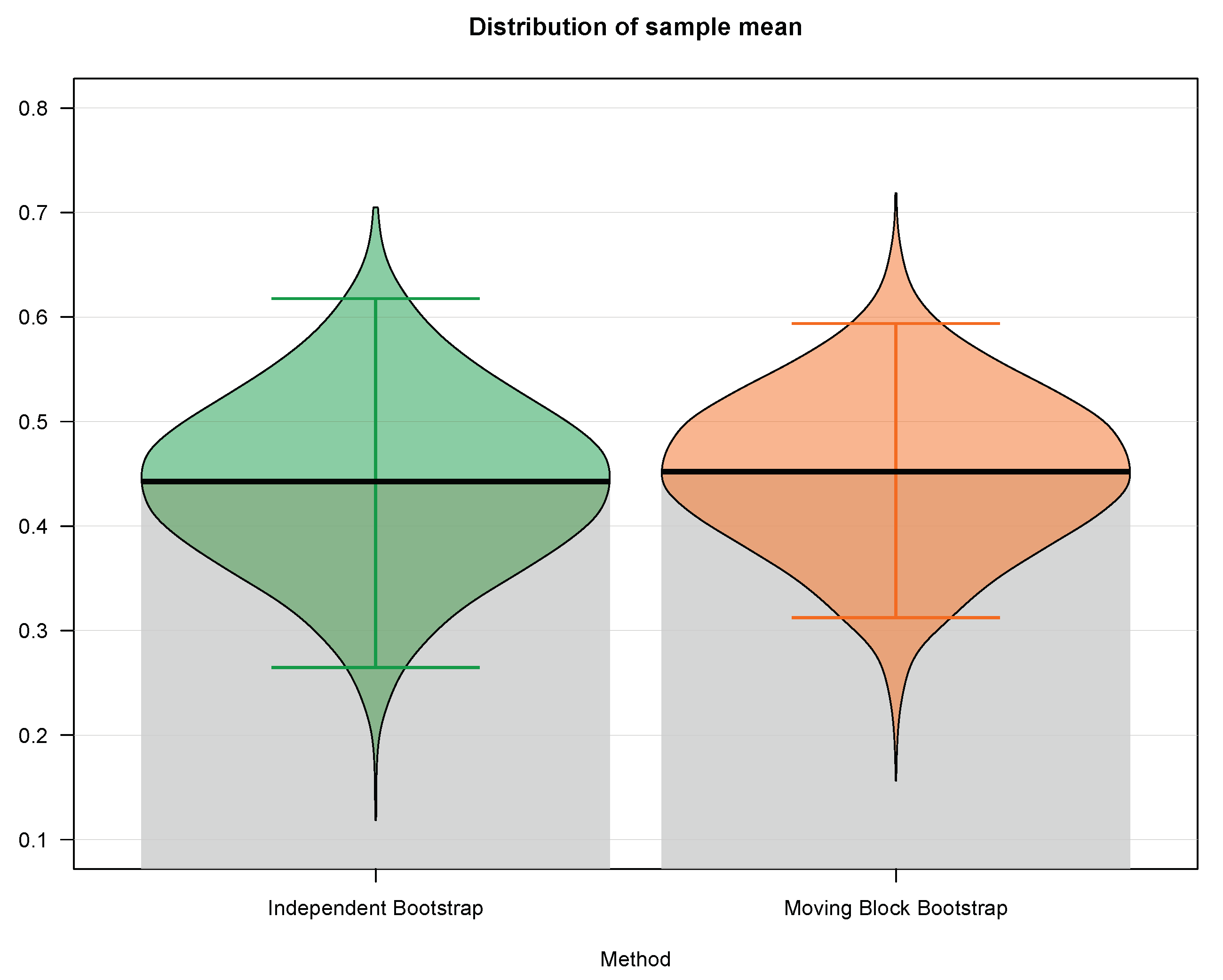
We utilize the independent bootstrap (ignoring the dependence among the responses) and the moving block bootstrap with the blocksize . The results for resampling the sample mean are shown in Table 1 and in Figure 1.
One may notice, from Table 1 as well as from Figure 1, that the difference between the 97.5th percentile and the 2.5th percentile, which serves as a 95% confidence interval, is narrower in case of the moving block bootstrap approach. Indeed, the 95% confidence interval based on independent bootstrap is [0.2647, 0.6176], whereas the 95% confidence interval based on moving block bootstrap is [0.3125, 0.5938]. Hence, the lengths of the confidence intervals are 0.3529 and 0.2813 for the independent and the moving block bootstrap, respectively, which yields approximately 20% reduction in the confidence interval’s length and, thus, an increase in estimation precision. In the end, the standard deviation for the independent bootstrap is 0.0851, whereas the standard deviation for the mooving block bootstrap drops down to 0.0764, which also provides an increase in precision by taking into account the underlying dependence among the data.
6.2. Insurance
In non-life insurance, the claims are traditionally split into the attritional and large claims, see, for example, [42]. One of the most fundamental tasks in non-life insurance, conducted on regular basis, is risk reserving assessment analysis, which amounts to predict the overall loss reserves to cover possible future claims. In order to do that, one firstly needs to estimate stochastically the distributional characteristics of the historical claims [43]. Here, we concentrate on estimation of the unknown mean for a reinsurance caped layer of large claims. Since the considered reinsurance layer will be bounded, there is no issue of assuming that the expectation of the underlying claims belonging to this layer exists.
We use the large fire insurance claims in Denmark from Thursday 3rd January 1980 until Monday 31st December 1990. The data called “Danish Fire Insurance Claims” were supplied by Mette Rytgaard of Copenhagen Re. They were described in [44] and can be freely downloaded from (https://tmsalab.github.io/edmdata/, accessed on 12 November 2022). Note that these data form an irregular time series, which does not contradict the notion of weak dependence. On contrary, the concept of mixing is very suitable for the unequally spaced time series [45]. We think of the reinsurance caped layer covering the large claims starting from 20M DKK (Danish crowns) up to 100M DKK, which consists n = 33 fire claims. The parameter of interest for the underlying unknown distribution is the mean. Again, it exists due to the fact that the layer is bounded from below as well as from above. Hence, the sample mean is the consistent and asymptotically normal estimator of the mean parameter. If the data are dependent and non-stationary (and, thus, not identically distributed), one cannot rely on normal asymptotics when constructing the confidence interval for the mean, because the corresponding limiting variance becomes unknown [46,47,48]. Therefore, the proper bootstrap method can provide a suitable solution.
The independent bootstrap (ignoring the dependence and non-stationarity among the fire claims) and the moving block bootstrap with the blocksize are applied. The results for resampling the sample mean are numerically displayed in Table 2. Additional to that, the empirical distributions of the sample mean based on the both resampling techniques together with the empirical distributional quantities from Table 2 are graphically visualized in Figure 2.
Table 2 as well as Figure 2 clearly reveal that the 95% confidence interval, which is the difference between the 97.5th percentile and the 2.5th percentile, is narrower in case of the moving block bootstrap procedure. Truly, the 95% confidence interval based on independent bootstrap is [27.94, 35.90], whereas the 95% confidence interval based on moving block bootstrap is [29.39, 35.38]. Hence, the lengths of the confidence intervals are 7.96 and 5.99 for the independent and the moving block bootstrap, respectively, which gives approximately 25% reduction in the confidence interval’s length. This provides an increase in estimation precision, which can be incorporated and employed in the reserving techniques for not independent and not identically distributed data, see [49,50,51,52]. On top of that, the standard deviation for the independent bootstrap is 2.054, whereas the standard deviation for the mooving block bootstrap drops down to 1.521, which again confirms an increase in accuracy by assuming the underlying dependence in the data.
7. Conclusions and Discussion
Asymptotic normality of the estimators or test statistics might be computationally unattainable and, hence, it can fail in practical applications. The discussed disadvantageous asymptotic properties lead to usage of the distributional-free resampling methods even for the IID observations. On top of that, the bootstrap procedures for a class of not independent and not identically distributed data are given together with their theoretical validity. There are three main methodological contributions to the bootstrap inference developed in this paper: (i) asymptotic closeness of the unknown stochastic quantities and their bootstrap counterparts is properly mathematically formalized; (ii) laws of large numbers for the bootstrapped -mixing and -mixing random variables and vectors are postulated and proved; (iii) central limit theorems for the bootstrapped NINID observations are provided, which serve as justifications of the popular computer intensive techniques. Lastly, the theoretically valid approaches are practically performed on the problems from psychometry and insurance.
The concept of weak dependence provides a very flexible framework and it allows to handle any autocorrelation structure for the observations, if the mixing conditions are satisfied. Furthermore, if the parameter of interest is not the mean, our developed methodology can still be useful. Suppose that the corresponding estimator of the unknown parameter can be somehow linearized and, thus, rewritten as a continuous functional of a mean of the random variables plus some remainder, which is negligible in probability. This can be achieved, for instance, through the stochastic Taylor expansion. Then, one may apply the derived bootstrap machinery on the mean from the continuous functional and, additionally, use the continuous mapping theorem to obtain validity for bootstrapping the parameter of interest.
Author Contributions
All the authors M.H., M.M., B.P., and M.P.–contributed equally. All authors have read and agreed to the published version of the manuscript.
Funding
The research of Martin Hrba, Matúš Maciak, and Michal Pešta was funded by the Czech Science Foundation project GAČR No. 21-13323S. The work of Barbora Peštová was supported by the Czech Science Foundation project GAČR No. 21-03658S.
Data Availability Statement
There are two datasets used in this paper and both are publicly available. The first dataset–Programme for International Student Assessment (PISA) 2012 U.S. Math Assessment–can be downloaded from https://tmsalab.github.io/edmdata/, accessed on 12 November 2022 [41]. The second dataset–Danish Fire Insurance Claims–can be downloaded from https://vincentarelbundock.github.io/, accessed on 12 November 2022 [44].
Acknowledgments
The authors would like to thank three anonymous referees for their constructive comments and valuable remarks that have significantly improved this paper.
Conflicts of Interest
The authors declare no conflict of interest.
Abbreviations
The following abbreviations are used in this manuscript:
| IID | Independent and identically distributed |
| NINID | Not independent and not identically distributed |
| LLN | Law of large numbers |
| SLLN | Strong law of large numbers |
| WLLN | Weak law of large numbers |
| BWLLN | Bootstrap weak law of large numbers |
| CLT | Central limit theorem |
| BCLT | Bootstrap central limit theorem |
Appendix A. Proofs
Proof of Lemma 1.
Proof of Theorem 1.
First, we show that
i.e., for arbitrary bounded continuous function f holds
Let be such arbitrary bounded continuous function. Now consider the function of a single argument . This will obviously be a bounded and continuous non-random function as well. By assumption (3), we will have that
However, the latter expression is equivalent to (A2). Therefore, we now know that conditioned on and approach each other in distribution -almost surely along .
Secondly, consider . This expression converges in probability to zero -almost surely due to Assumption (4). Thus, we have demonstrated two facts: (A1) and
Since each bounded continuous function is bounded Lipschitz and vice versa, consider any bounded Lipschitz function :
Take some arbitrary and majorize
Hence,
We take the limit in this expression as . Since (A4) holds for arbitrary , the second term will go to zero -almost surely due to (A3) and Definition 3. The third term (does not depend on ) will also converge to zero -almost surely by (A2). Thus,
Since was arbitrary, we conclude that the limit must in fact be equal to zero -almost surely. Therefore, (i) is proved.
In order to prove result (viii), consider again . This expression converges in probability in probability to zero due to assumption (6). Thus
Which can be rewritten according to Definition 3 as
Let us fix . Similarly as in the proof of part (i), it can be demonstrated that
When convergence -almost surely is just replaced by convergence in probability . Indeed, using inequality (A4), we get for arbitrary (and above chosen fixed and sufficiently small )
If we take the limit in previous inequality as n goes to infinity, the first term is zero and the second term will go to zero due to (A5) and Definition 3. The third term will also converge to zero by (A6). Thus
Since was arbitrary, (viii) is proved.
Assertions (ii)–(vii) are just corollaries of (i), when continuous mapping theorem (see, e.g., Theorems 2 and 3 [55]) is applied. Similarly, assertions (ix)–(xiv) are consequences of (viii). □
Proof of Lemma 2.
See [56] (Theorem 1). □
Proof of Lemma 3.
See [57] (Theorem 4.1). □
Proof of Lemma 4.
See [23] (Theorem 5.2). □
Proof of Corollary 1.
Since a functional distributional limit (a convergence in Skorokhod space) implies the pointwise distributional limit, this corollary is just a special case of Lemma 5, when is considered. □
Proof of Lemma 6.
See [59] (Corollary 4). □
Proof of Corollary 2.
The first step is to show that Conditions (20) and (21) implies the so-called Lyapunov condition, i.e., having fixed :
Now, the Lyapunov condition holds and we fix . Since implies , we obtain
□
Proof of Theorem 2.
The SLLN applied for independent random variables together with Assumption (23) lead to
Markov’s inequality with (23) implies uniform equiboundedness in probability of . The conditional variance of the bootstrapped sample mean goes to zero as n increases to infinity, because
Hence, the weak law of large numbers in the “starred” world (for resampled variables) provides
Because are conditionally IID. □
Proof of Theorem 3.
The sequence is uniformly bounded in probability , because (25) is assumed. By the assumptions for and Lemma 2, it is known that a SLLN holds for the sample mean . By Corollary A2 from [12], it follows that
Thus the claim holds due to Lemma A1 by [12], where
□
Proof of Theorem 4.
The proof is the same as the proof of previous Lemma 3 except one detail–the SLLN for -mixing (Lemma 3) has to be applied instead of Lemma 2 for -mixing. □
Proof of Theorem 5.
See [60]. □
Proof of Theorem 6.
The Lyapunov condition for sequence of random variables is satisfied due to (28) and (29), i.e., for fixed :
Thereupon, the CLT for holds and
Henceforth, to prove this theorem, it suffices to show the following three statements:
- (i)
- (ii)
- (iii)
Proving (iii) is trivial, because the bootstrapped variables are conditionally IID and, therefore,
Let us calculate the conditional variance of the bootstrapped :
The strong law of large numbers for independent non-identically distributed random variables with (28) provide
and
The last result of the SLLN is true, because (28) implies
Thus (ii) is proved.
The Berry–Esseen-Katz Theorem 5 with for the bootstrapped sequence of IID (with respect to ) random variables results into
where is an absolute constant.
The Minkowski inequality and Jensen’s inequality provide an upper bound for the nominator from the right-hand side of (A7):
The right-hand side of the previously derived upper bound is uniformly bounded in probability , because of Markov’s inequality and (28). In very deed, for fixed
and
Proof of Theorem 7.
According to Cramér–Wold theorem, it is sufficient to ensure that all the assumptions of one-dimensional bootstrap CLT 6 are valid for any linear combination of the elements of random vector .
For arbitrary fixed using Jensen’s inequality, we get
Similar situation arises, when assumption (34) implies assumption (29) for such an arbitrary linear combination, i.e., positive definiteness of matrix yields
Finally, we need to realize that (34) holds, (35) has already been proved above, are conditionally IID, and
□
Proof of Theorem 8.
The proof of this theorem goes along the lines the proof of Theorem 6 except three facts: the bootstrap WLLN for -mixing–Lemma 3 is used; the CLT for -mixing–Corollary 1 is employed; and another covariance inequality is applied, i.e., Lemma 1.2.5 by [26]. □
Proof of Theorem 9.
The proof of this theorem remains almost the same as the proof of Theorem 8 with the only exception that the following tools have to be used instead: the CLT for -mixing observations, i.e., Corollary 2; a different covariance inequality, i.e., Lemma 1.2.8 by [26]; and a suitable bootstrap WLLN, i.e., Lemma 4. □
References
- Efron, B. Bootstrap methods: Another look at the jackknife. Ann. Stat. 1979, 7, 1–26. [Google Scholar]
- Bickel, P.J.; Freedman, D.A. Some asymptotic theory for the bootstrap. Ann. Stat. 1981, 9, 1196–1217. [Google Scholar] [CrossRef]
- Efron, B.; Tibshirani, R. An Introduction to the Bootstrap; Chapman and Hall: London, UK, 1990. [Google Scholar]
- Efron, B.; Hastie, T. Computer Age Statistical Inference, Student ed.; Cambridge University Press: Cambridge, UK, 2013. [Google Scholar]
- Hall, P. The Bootstrap and Edgeworth Expansion; Springer: New York, NY, USA, 2013. [Google Scholar]
- Lahiri, S.N. Resampling Methods for Dependent Data; Springer: New York, NY, USA, 2003. [Google Scholar]
- Politis, D.N.; Romano, J.P.; Wolf, M. Subsampling; Springer: New York, NY, USA, 1999. [Google Scholar]
- Künsch, H.R. The jacknife and the bootstrap for general stationary observations. Ann. Stat. 1989, 17, 1217–1241. [Google Scholar] [CrossRef]
- Liu, R.Y.; Singh, K. Moving blocks jackknife and bootstrap capture weak dependence. In Proceedings of the Exploring the Limits of Bootstrap; Lapage, R., Billard, L., Eds.; Wiley: New York, NY, USA, 1992; pp. 225–248. [Google Scholar]
- Lahiri, S.N. Non-strong mixing autoregressive processes. Stat. Probabil. Lett. 1991, 11, 335–341. [Google Scholar]
- Politis, D.N.; Romano, J.P. A general resampling scheme for triangular arrays of α-mixing random variables with application to the problem of spectral density estimation. Ann. Stat. 1992, 20, 1985–2007. [Google Scholar] [CrossRef]
- Fitzenberger, B. The moving block bootstrap and robust inference for linear least squares and quantile regression. J. Econometr. 1998, 82, 235–287. [Google Scholar] [CrossRef]
- Maciak, M.; Peštová, B.; Pešta, M. Structural breaks in dependent, heteroscedastic, and extremal panel data. Kybernetika 2019, 54, 1106–1121. [Google Scholar] [CrossRef]
- Pesarin, F.; Salmaso, L. Permutation Tests for Complex Data: Theory, Applications and Software; Wiley: New York, NY, USA, 2010. [Google Scholar]
- Pešta, M. Total least squares and bootstrapping with application in calibration. Statistics 2013, 47, 966–991. [Google Scholar] [CrossRef]
- Pešta, M. Block bootstrap for dependent errors-in-variables. Commun. Stat. A-Theory 2017, 46, 1871–1897. [Google Scholar] [CrossRef]
- Hall, P.; Horowitz, J.L.; Jing, B.Y. On blocking rules for the bootstrap with dependent data. Biometrika 1995, 82, 561–574. [Google Scholar]
- Politis, D.N.; White, H. Automatic block-length selection for the dependent bootstrap. Econometr. Rev. 2004, 23, 53–70. [Google Scholar] [CrossRef]
- Lahiri, S.; Furukawa, K.; Lee, Y.D. A nonparametric plug-in rule for selecting optimal block lengths for block bootstrap methods. Stat. Methodol. 2007, 4, 292–321. [Google Scholar] [CrossRef]
- Kirch, C. Resampling Methods for the Change Analysis of Dependent Data. Ph.D. Thesis, University of Cologne, Cologne, Germany, 2006. [Google Scholar]
- Peštová, B.; Pešta, M. Abrupt change in mean using block bootstrap and avoiding variance estimation. Comput. Stat. 2018, 33, 413–441. [Google Scholar]
- Billingsley, P. Convergence of Probability Measures, 2nd ed.; John Wiley & Sons: New York, NY, USA, 1999. [Google Scholar]
- Bradley, R.C. Basic properties of strong mixing conditions. A survey and some open questions. Probab. Surv. 2005, 2, 107–144. [Google Scholar]
- Gijbels, I.; Omelka, M.; Pešta, M.; Veraverbeke, N. Score tests for covariate effects in conditional copulas. J. Multivar. Anal. 2017, 159, 111–133. [Google Scholar]
- Rosenblatt, M. A central limit theorem and a strong mixing condition. Proc. Natl. Acad. Sci. USA 1956, 42, 43–47. [Google Scholar] [CrossRef]
- Lin, Z.; Lu, C. Limit Theory for Mixing Dependent Random Variables; Springer: New York, NY, USA, 1997. [Google Scholar]
- Ibragimov, I.A. Some limit theorems for stochastic processes stationary in the strict sense. Dokl. Akad. Nauk. SSSR 1959, 125, 711–714. (In Russian) [Google Scholar]
- Pešta, M. Asymptotics for weakly dependent errors-in-variables. Kybernetika 2013, 49, 692–704. [Google Scholar]
- Anderson, T.W. An Introduction to Multivariate Statistical Analysis; John Wiley & Sons: New York, NY, USA, 1958. [Google Scholar]
- Billingsley, P. Convergence of Probability Measures, 1st ed.; John Wiley & Sons: New York, NY, USA, 1968. [Google Scholar]
- Doob, J.L. Stochastic Processes; John Wiley & Sons: New York, NY, USA, 1953. [Google Scholar]
- Ibragimov, I.A.; Linnik, Y.V. Independent and Stationary Sequences of Random Variables; Wolters-Noordhoff: Amsterdam, The Netherlands, 1971. [Google Scholar]
- Rosenblatt, M. Markov Processes: Structure and Asymptotic Behavior; Springer: Berlin/Heidelberg, Germany, 1971. [Google Scholar]
- Antoch, J.; Hušková, M.; Prášková, Z. Effect of dependence on statistics for determination of change. J. Stat. Plan. Infer. 1997, 60, 291–310. [Google Scholar] [CrossRef]
- Andrews, D.W.K. Heteroskedasticity and autocorrelation consistent covariance matrix estimation. Econometrica 1991, 59, 817–858. [Google Scholar] [CrossRef]
- Belyaev, Y.K. Bootstrap, Resampling and Mallows Metric. Lecture Notes 1; Institute of Mathematical Statistics, UmeåUniversity: Umeå, Sweden, 1995. [Google Scholar]
- Singh, K. On the asymptotic accuracy of Efron’s bootstrap. Ann. Stat. 1981, 9, 1187–1195. [Google Scholar] [CrossRef]
- Peštová, B.; Pešta, M. Testing structural changes in panel data with small fixed panel size and bootstrap. Metrika 2015, 78, 665–689. [Google Scholar]
- Peštová, B.; Pešta, M. Erratum to: Testing structural changes in panel data with small fixed panel size and bootstrap. Metrika 2016, 79, 237–238. [Google Scholar] [CrossRef] [Green Version]
- Peštová, B.; Pešta, M. Change point estimation in panel data without boundary issue. Risks 2017, 5, 7. [Google Scholar] [CrossRef] [Green Version]
- Culpepper, S.A.; Balamuta, J.J. Inferring latent structure in polytomous data with a higher-order diagnostic model. Multivar. Behav. Res. 2021, 1–19. [Google Scholar] [CrossRef]
- Maciak, M.; Mizera, I.; Pešta, M. Functional profile techniques for claims reserving. ASTIN Bull. 2022, 52, 449–482. [Google Scholar]
- Gerthofer, M.; Pešta, M. Stochastic claims reserving in insurance using random effects. Prague Econ. Pap. 2017, 26, 542–560. [Google Scholar] [CrossRef] [Green Version]
- McNeil, A.J. Estimating the tails of loss severity distributions using extreme value theory. ASTIN Bull. 1997, 27, 117–137. [Google Scholar] [CrossRef] [Green Version]
- Pešta, M. Changepoint in error-prone relations. Mathematics 2021, 9, 89. [Google Scholar] [CrossRef]
- Pešta, M.; Wendler, M. Nuisance-parameter-free changepoint detection in non-stationary series. Test 2020, 29, 379–408. [Google Scholar]
- Maciak, M.; Pešta, M.; Peštová, B. Changepoint in dependent and non-stationary panels. Stat. Pap. 2020, 61, 1385–1407. [Google Scholar] [CrossRef]
- Pešta, M.; Peštová, B.; Maciak, M. Changepoint estimation for dependent and non-stationary panels. Appl. Math.-Czech. 2020, 65, 299–310. [Google Scholar] [CrossRef]
- Pešta, M.; Hudecová, Š. Asymptotic consistency and inconsistency of the chain ladder. Insur. Math. Econ. 2012, 51, 472–479. [Google Scholar] [CrossRef]
- Hudecová, Š.; Pešta, M. Modeling dependencies in claims reserving with GEE. Insur. Math. Econ. 2013, 53, 786–794. [Google Scholar]
- Pešta, M.; Okhrin, O. Conditional least squares and copulae in claims reserving for a single line of business. Insur. Math. Econ. 2014, 56, 28–37. [Google Scholar] [CrossRef] [Green Version]
- Maciak, M.; Okhrin, O.; Pešta, M. Infinitely stochastic micro reserving. Insur. Math. Econ. 2021, 100, 30–58. [Google Scholar]
- Belyaev, Y.K.; Sjöstedt-de Luna, S. Weakly approaching sequences of random distributions. J. Appl. Probab. 2000, 37, 807–822. [Google Scholar] [CrossRef] [Green Version]
- Zagdaǹski, A. On the construction and properties of bootstrap-t prediction intervals for stationary time series. Probab. Math. Statist. 2005, 25, 133–153. [Google Scholar]
- van der Vaart, A.W. Asymptotic Statistics; Cambridge University Press: New York, NY, USA, 1998. [Google Scholar]
- Chen, X.; Wu, Y. Strong law for mixing sequence. Acta Math. Appl. Sin. 1989, 5, 367–371. [Google Scholar]
- Xuejun, W.; Shuhe, H.; Yan, S.; Wenzhi, Y. Moment inequalities for φ-mixing sequences and its applications. J. Inequal. Appl. 2009, 2009, 12. [Google Scholar] [CrossRef] [Green Version]
- Herrndorf, N. A functional central limit theorem for strongly mixing sequence of random variables. Probab. Theory Relat. Fields 1985, 69, 541–550. [Google Scholar] [CrossRef]
- Utev, S.A. The central limit theorem for φ-mixing arrays of random variables. Theory Probab. Appl. 1990, 35, 131–139. [Google Scholar] [CrossRef]
- Katz, M.L. Note on the Berry–Esseen theorem. Ann. Math. Stat. 1963, 34, 1107–1108. [Google Scholar]
Figure 1.
Empirical distributions of the sample mean based on the independent bootstrap (green—incorrect approach) against moving block bootstrap (orange—proper approach) for the correct/incorrect answers by a subject from the Programme for International Student Assessment (PISA) 2012—U.S. Math Assessment.

Figure 2.
Empirical distributions of the sample mean based on the independent bootstrap (blue—incorrect approach) against moving block bootstrap (red—proper approach) for the Danish Fire Insurance Claims belonging to the reinsurance layer starting from 20M DKK (Danish crowns) up to 100M DKK.
Figure 2.
Empirical distributions of the sample mean based on the independent bootstrap (blue—incorrect approach) against moving block bootstrap (red—proper approach) for the Danish Fire Insurance Claims belonging to the reinsurance layer starting from 20M DKK (Danish crowns) up to 100M DKK.


Table 1.
Empirical distributional quantities of the sample mean based on the independent bootstrap (incorrect approach) against moving block bootstrap (proper approach) for the correct/incorrect answers by a subject from the Programme for International Student Assessment (PISA) 2012–U.S. Math Assessment; number of observations n = 34.
| Empirical Quantity | Independent Bootstrap | Moving Block Bootstrap |
|---|---|---|
| th percentile | 0.2647 | 0.3125 |
| First quartile | 0.3824 | 0.4062 |
| Median | 0.4412 | 0.4375 |
| Third quartile | 0.5000 | 0.4999 |
| 97.5th percentile | 0.6176 | 0.5938 |
Table 2.
Empirical distributional quantities of the sample mean based on the independent bootstrap (blue—incorrect approach) against moving block bootstrap (red—proper approach) for the Danish Fire Insurance Claims belonging to the reinsurance layer starting from 20M DKK (Danish crowns) up to 100M DKK; number of observations n = 33.
| Empirical Quantity | Independent Bootstrap | Moving Block Bootstrap |
|---|---|---|
| 2.5th percentile | 27.94 | 29.39 |
| First quartile | 30.28 | 31.20 |
| Median | 31.64 | 32.20 |
| Third quartile | 33.08 | 33.29 |
| 97.5th percentile | 35.90 | 35.38 |
Publisher’s Note: MDPI stays neutral with regard to jurisdictional claims in published maps and institutional affiliations. |
© 2022 by the authors. Licensee MDPI, Basel, Switzerland. This article is an open access article distributed under the terms and conditions of the Creative Commons Attribution (CC BY) license (https://creativecommons.org/licenses/by/4.0/).
Share and Cite
MDPI and ACS Style
Hrba, M.; Maciak, M.; Peštová, B.; Pešta, M. Bootstrapping Not Independent and Not Identically Distributed Data. Mathematics 2022, 10, 4671. https://doi.org/10.3390/math10244671
AMA Style
Hrba M, Maciak M, Peštová B, Pešta M. Bootstrapping Not Independent and Not Identically Distributed Data. Mathematics. 2022; 10(24):4671. https://doi.org/10.3390/math10244671
Chicago/Turabian StyleHrba, Martin, Matúš Maciak, Barbora Peštová, and Michal Pešta. 2022. "Bootstrapping Not Independent and Not Identically Distributed Data" Mathematics 10, no. 24: 4671. https://doi.org/10.3390/math10244671
Note that from the first issue of 2016, this journal uses article numbers instead of page numbers. See further details here.