Cosmic-Ray Anisotropies in Right Ascension Measured by the Pierre Auger Observatory

The distribution of cosmic-ray (CR) arrival directions is expected to provide essential clues to understanding the CR origin. Being charged particles, they are significantly deflected by the magnetic fields present in our galaxy (Haverkorn 2015) and, for those arriving from outside it, also by the extragalactic magnetic fields (Feretti et al. 2012). Since the deflections get smaller for increasing rigidities, it is only at the highest energies that one may hope to observe localized flux excesses associated with individual CR sources. On the other hand, as the energies lower and the deflections become large, the propagation eventually becomes diffusive and it is likely that only large-scale patterns, such as a dipolar flux modulation, may be detectable. However, the small amplitudes of these anisotropies make their observation quite challenging.

Due to the Earth's rotation, CR observatories running for long periods of time have an almost uniform exposure in R.A. This enables them to achieve a high sensitivity to the modulation of the flux in this angular coordinate. In particular, for a dipolar CR flux the first-harmonic modulation in R.A. provides a direct measurement of the projection of the dipole in the equatorial plane, ${{\boldsymbol{d}}}_{\perp }$. The possible sources of systematic uncertainties that could affect these measurements, such as those from remaining nonuniformities of the exposure or those related to the effects of atmospheric variations, can often be accounted for. Even when this is not possible, as can happen when the trigger efficiency of the array is small, methods that are insensitive to these systematic effects can be adopted to reconstruct ${{\boldsymbol{d}}}_{\perp }$, although they have a somewhat reduced sensitivity to the modulations. On the other hand, at low energies the number of events detected is large, what tends to enhance the statistical sensitivity of the measurements.

The projection of the dipole along the Earth rotation axis d_z can, in principle, be reconstructed from the study of the azimuthal modulation of the CR fluxes. This requires accounting in detail for the effects of the geomagnetic field on the air showers, which can affect the reconstruction of the CR energies in an azimuthally dependent way. Also, the presence of a tilt of the array can induce a spurious contribution to d_z. When the trigger efficiency of the array is small, these effects may lead to systematic uncertainties that cannot be totally corrected for, particularly given the azimuthal dependence of the trigger efficiency arising from the actual geometry of the surface detector array of the Pierre Auger Observatory. Due to these limitations, we will here restrict our analysis to the determination of ${{\boldsymbol{d}}}_{\perp }$ through the study of the distribution in R.A. of the events recorded in different energy bins. We note that the determination of d_z for energies E ≥ 4 EeV, for which that detector has full efficiency for zenith angles up to 80°, was discussed in detail in The Pierre Auger Collaboration (2015a, 2017a, 2018).

At E ≥ 8 EeV, a significant first-harmonic modulation in R.A., corresponding to an amplitude d_⊥ ∼ 6%, has been detected by the Pierre Auger Observatory (The Pierre Auger Collaboration 2017a). The reconstructed direction of the three-dimensional dipole suggests a predominant extragalactic origin of the CR anisotropies at energies above 4 EeV, and the dipolar amplitudes obtained in different bins show a growing trend with increasing energies (The Pierre Auger Collaboration 2017a, 2018).

The phase in R.A. of the dipolar modulation of the flux determined above 8 EeV is α_d ≃ 100°. This is nearly opposite to the phases measured at PeV energies by IceCube and IceTop (IceCube Collaboration 2012, 2016), which lie not far from the Galactic center direction which is at α_GC = −94°. Also the KASCADE-Grande measurements, involving CR energies from few PeV up to few tens of PeV, lead to phases lying close to the R.A. of the Galactic center, even though the measured amplitudes are not statistically significant (KASCADE-Grande Collaboration 2019).⁹⁷ All this is in agreement with the expectation that for energies above that of the knee of the CR spectrum, which corresponds to the steepening taking place at ∼4 PeV, the outward diffusive escape of the CRs produced in the Galaxy should give rise to a dipolar flux component having its maximum not far from the Galactic center direction. Also at energies above few EeV, where the propagation would become more rectilinear, a continuous distribution of Galactic sources should give rise to a dipolar component not far from the GC direction (The Pierre Auger Collaboration 2018). Departures from these behaviors could, however, result if the CR source distribution is not symmetric with respect to the Galactic center (such as in the presence of a powerful nearby CR source), in the presence of drift motions caused by the regular Galactic magnetic field components (Ptuskin et al. 1993), or when the contribution from the extragalactic component becomes sizable. Note that the expected direction of a dipole of extragalactic origin will depend on the (unknown) distribution of the CR sources and on the effects of the deflections caused by the Galactic magnetic field, as was discussed in detail in The Pierre Auger Collaboration (2018).

The change from a Galactic CR origin toward a predominantly extragalactic origin is expected to take place somewhere above the knee. More precise measurements of the large-scale anisotropies, filling the gap between the IceCube/IceTop or KASCADE-Grande measurements and the dipole determined by the Pierre Auger Observatory above 8 EeV, should provide information about this transition. In fact, although at energies below 8 EeV the reported dipolar amplitudes are not significant, indications that a change in the phase of the anisotropies in R.A. takes place around few EeV are apparent in the Pierre Auger Observatory measurements (The Pierre Auger Collaboration 2011a, 2012, 2013; Sidelnik 2013; Al Samarai 2016). One has to keep in mind in this discussion that the energy at which the total anisotropy becomes of predominantly extragalactic origin may be different from the energy at which the CR flux becomes of predominantly extragalactic origin, since the intrinsic anisotropies of each component are likely different.

We present here an update of the measurements of the large-scale anisotropies that are sensitive to the equatorial component of a dipole, for the whole energy range from ∼0.03 EeV up to ≥32 EeV, covering more than three decades of energy. The results above 4 EeV are an update of those presented in The Pierre Auger Collaboration (2018), including two more years of data, corresponding to an increase in the exposure by 20%. At lower energies, we provide a major update of the latest published results (Al Samarai 2016), with 50% more exposure for the SD1500 array and twice as much for the SD750 array. At energies below 2 EeV, possible systematic effects related to the reduced trigger efficiency could be significant. To study the modulation in R.A. in this regime we have then to resort to the "east–west" method, which has larger associated uncertainties but is not affected by most of the systematic effects (Nagashima et al. 1989; Bonino et al. 2011). At energies below 0.25 EeV, it proves convenient to use the data from the subarray of detectors with 750 m spacing which, although being much smaller, can detect a larger number of events at these energies.

The Pierre Auger Observatory (The Pierre Auger Collaboration 2015b), located near the city of Malargüe in western Argentina (at latitude 352 South), is the largest existing CR observatory. Its surface detector array (SD) consists of water-Cerenkov detectors having each one 12 tonnes of ultra-pure water viewed by three 9 inch phototubes. The main array, SD1500, consists of detectors distributed on a triangular grid with separations of 1500 m that span an area of 3000 km². A smaller subarray, SD750, covers an area of 23 km² with detectors separated by 750 m, making it sensitive also to smaller CR energies. These arrays sample the secondary particles of the air showers reaching ground level. In addition, the fluorescence detector (FD) consists of 27 telescopes that overlook the SD array. The FD can determine the longitudinal development of the air showers by observing the UV light emitted by atmospheric nitrogen molecules excited by the passage of the charged particles of the shower. This fluorescence light can be detected during clear moonless nights, with a corresponding duty cycle of about 15% (The Pierre Auger Collaboration 2015b). The SD arrays have instead a continuous operation, detecting events with a duty cycle close to 100%. They also have a more uniform (and simpler to evaluate) exposure. This is why the studies of the large-scale anisotropies that we perform here are based on the much larger number of events recorded by the surface arrays.

For the SD1500 array, the data set considered in this work includes events with energies above 0.25 EeV that were detected from 2004 January 1 up to 2018 August 31. For energies below 4 EeV, it includes events with zenith angles up to 60°, allowing coverage of 71% of the sky, and the quality trigger applied requires that all the six detectors surrounding the one with the largest signal be active at the time the event is detected. For energies above 4 EeV, more inclined events can be reliably reconstructed (The Pierre Auger Collaboration 2014b) and hence the zenith-angle range is extended up to 80°, allowing coverage of 85% of the sky. Moreover, given that at these energies the number of detectors triggered by each shower is large (4 or more detectors for more than 99% of the events), we also include in this case events passing a relaxed trigger condition, allowing that one of the six detectors that are neighbors to the one with the largest signal be missing or not functioning, provided that the reconstructed shower core be contained inside a triangle of nearby active detectors (The Pierre Auger Collaboration 2017a). The integrated exposure of the array for θ ≤ 60° and using the strict trigger selection is 60,700 km² sr yr, while that for θ ≤ 80° and relaxing the trigger is 92,500 km² sr yr.

The CR arrival directions are reconstructed from the timing of the signals in the different triggered stations, and the angular resolution is better than 16 (The Pierre Auger Collaboration 2015b), so that it has negligible impact on the reconstruction of the dipole. The energies of the events with θ ≤ 60° are assigned in terms of the reconstructed signals at a reference distance from the shower core of 1000 m. They are corrected for atmospheric effects, accounting for the pressure and air density variations following The Pierre Auger Collaboration (2017b), as well as for geomagnetic effects, following The Pierre Auger Collaboration (2011b). The inclined events, whose signals are dominantly produced by the muonic component of the showers, have a negligible dependence on atmospheric variations, while geomagnetic effects are already taken into account in their reconstruction (The Pierre Auger Collaboration 2014b). Their energies are assigned in terms of the estimated muon number at ground level. The SD1500 array has full trigger efficiency for E ≥ 2.5 EeV if one considers events with θ ≤ 60°, and for E ≥ 4 EeV for events with θ ≤ 80°. The energies of the CRs are calibrated using the hybrid events measured simultaneously by the SD and FD detectors, in the regimes of full trigger efficiency. For lower energies, in which case we consider events with θ ≤ 60°, the energy assignment is performed using the extrapolation of the corresponding calibration curve. The energy resolution for events with θ ≤ 60° is about 7% above 10 EeV, and degrades for lower energies, reaching about 20% at 1 EeV, while the systematic uncertainty in the energy scale is 14% (see Verzi 2019 for details). The more inclined events have an energy resolution of 19%, with a similar systematic uncertainty (The Pierre Auger Collaboration 2014b).

For energies below 0.25 EeV, and down to ∼0.03 EeV (below which the trigger efficiency is tiny), we use the events from the denser and smaller SD750 array, since the accumulated statistics is larger. The data set comprises events with zenith angles up to 55° detected from 2012 January 1 up to 2018 August 31. The trigger applied requires that all six detectors around the one with the largest signal be functioning and the associated exposure is 234 km² sr yr. The energies are assigned in terms of the reconstructed signals at a reference distance from the shower core of 450 m. They are corrected for atmospheric effects following The Pierre Auger Collaboration (2017b). The SD750 array has full trigger efficiency for E ≥ 0.3 EeV if one considers events with θ ≤ 55° (The Pierre Auger Collaboration 2015b). The energies are calibrated with hybrid events observed in the regime of full trigger efficiency and below that threshold the energy assignment is performed on the basis of the extrapolation of the corresponding calibration curve. At 0.3 EeV the energy resolution is about 18% (Coleman 2019).

The weighted first-harmonic analysis in the R.A. angle α, often referred to as Rayleigh analysis, provides the Fourier coefficients as

$$\begin{eqnarray}&&a=\displaystyle \frac{2}{{ \mathcal N }}\sum _{i=1}^{N}{w}_{i}\cos {\alpha }_{i},\,\,\,\,\,\,b=\displaystyle \frac{2}{{ \mathcal N }}\sum _{i=1}^{N}{w}_{i}\sin {\alpha }_{i},\end{eqnarray} \tag{ 1 }$$

where the sums run over all N detected events. The weights w_i, which are of order unity, account for the effects of the nonuniformities in the exposure as a function of time, with the normalization factor being ${ \mathcal N }\equiv {\sum }_{i}{w}_{i}$. The amplitude and phase of the first-harmonic modulation are given by $r=\sqrt{{a}^{2}+{b}^{2}}$ and $\varphi =\arctan (b/a)$. The probability to obtain an amplitude larger than the one measured as a result of a fluctuation from an isotropic distribution is $P(\geqslant r)=\exp (-{ \mathcal N }{r}^{2}/4)$. To obtain the weights, we permanently monitor the number of active unitary detector cells, corresponding to the number of active detectors that are surrounded by an hexagon of working detectors or, when considering the relaxed trigger condition above 4 EeV, we also account for detector configurations with only five active detectors around the central one. We obtain from this the exposure of the Auger Observatory in bins of R.A. of the zenith of the array, α⁰. This angle is given by ${\alpha }^{0}({t}_{i})\,\equiv 2\pi {t}_{i}/{T}_{s}\,(\mathrm{mod}\,2\pi )$, with the origin of time being taken such that α⁰(0) = 0. The sidereal-time period, T_s ≃ 23.934 hr, corresponds to one extra cycle per year with respect to the solar frequency. The fraction of the total exposure that is associated to a given α⁰ bin, taken to be of 125 width (5 minutes), is proportional to the total number of unitary cells in that bin, N_cell(α⁰). The weights w_i account for the relative variations of N_cell as a function of α⁰, i.e.,

$$\begin{eqnarray}&&{w}_{i}={\left(\displaystyle \frac{{N}_{\mathrm{cell}}({\alpha }^{0}({t}_{i}))}{\langle {N}_{\mathrm{cell}}\rangle }\right)}^{-1},\end{eqnarray} \tag{ 2 }$$

with $\langle {N}_{\mathrm{cell}}\rangle =1/(2\pi ){\int }_{0}^{2\pi }d{\alpha }^{0}\,{N}_{\mathrm{cell}}({\alpha }^{0})$. Including these weights in the Fourier coefficients eliminates the spurious contribution to the amplitudes associated to the nonuniform exposure in R.A.

We note that if one were to consider periods of only a few months, the resulting modulation of N_cell(α⁰) could amount to an effect of a few percent on the modulation in R.A. of the event rates. However, after considering several years, the modulations that appear on shorter timescales tend to get averaged out, with the surviving effects being now typically at the level of about ±0.5%. The effects of the tilt of the SD array (The Pierre Auger Collaboration 2012), which is inclined on average by ∼02 toward ϕ ≃ −30° (i.e., toward the southeast), can also be accounted for by adding an extra factor in the weights (The Pierre Auger Collaboration 2018). However, this is actually only relevant when performing the Fourier analysis in the azimuth variable ϕ, something we will not perform here.

When the triggering of the array is not fully efficient, there are additional systematic effects related to the interplay between the atmospheric effects in the air-shower development and the energy-dependent trigger efficiency. In particular, changes in the air density modify the Molière radius determining the lateral spread of the electromagnetic component of the showers. The fall-off of the signal at ground level is preferentially harder under hot weather conditions and steeper under cold ones. The detection efficiency of the SD is thus expected to follow these variations to some extent, being on average larger when the weather is hot than when it is cold. As a consequence, one could expect that, at energies below full trigger efficiency, a spurious modulation could appear at the solar frequency.

Moreover, we have found that the amplitude of the modulation of the rates at the antisidereal frequency, which is that corresponding to one cycle less per year than the solar frequency, suggests that spurious unaccounted effects become relevant below 2 EeV. In particular, the Fourier amplitude corresponding to the antisidereal time period T_as = 24.066 hr in the bin [1, 2] EeV is r = 0.005. This has a probability of arising as a fluctuation of less than 0.1%. A nonnegligible antisidereal amplitude could for instance appear in the presence of daily and seasonal systematic effects which are not totally accounted for. Since in this case comparable spurious amplitudes could be expected in the sidereal and antisidereal sidebands (Farley & Storey 1954), we only use the Rayleigh method described before in the bins above 2 EeV. We have checked that in the bins above 2 EeV the amplitudes at both the solar and antisidereal frequencies are consistent with being just due to fluctuations, so that there are no signs indicating that surviving systematic effects could be present at the sidereal frequency at these energies (see Table 2 in the Appendix).⁹⁸ Alternatively, one can use for the energies below 2 EeV the differential east–west (EW) method (Bonino et al. 2011), which is based on the difference between the counting rates of the events measured from the east sector and those from the west sector. Since the exposure is the same for events coming from the east and for those coming from the west,⁹⁹ and also the spurious modulations due to the atmospheric effects are the same in both sectors, the relative difference between both rates, $(E-W)/(E+W)$, is not sensitive to these experimental and atmospheric systematic effects. This allows one to reconstruct in a clean way the modulation of the rate itself, without the need to apply any correction but at the expense of a reduced sensitivity to the amplitude of the CR flux modulations.

In this approach (Bonino et al. 2011), the first-harmonic amplitude and phase are calculated using a slightly modified Fourier analysis that accounts for the subtraction of the western sector from the eastern one. The Fourier coefficients are defined as

$$\begin{eqnarray}\begin{array}{rcl}{a}_{\mathrm{EW}} & = & \displaystyle \frac{2}{N}\sum _{i=1}^{N}\cos ({\alpha }^{0}({t}_{i})-{\xi }_{i}),\\ {b}_{\mathrm{EW}} & = & \displaystyle \frac{2}{N}\sum _{i=1}^{N}\sin ({\alpha }^{0}({t}_{i})-{\xi }_{i}),\end{array}\end{eqnarray} \tag{ 3 }$$

where ξ_i = 0 for events coming from the east and ξ_i = π for those coming from the west, so as to easily implement the subtraction of data from the two hemispheres.

In the case in which the dominant contribution to the flux modulation is purely dipolar, the amplitude ${r}_{\mathrm{EW}}\,=\sqrt{{a}_{\mathrm{EW}}^{2}+{b}_{\mathrm{EW}}^{2}}$ and phase ${\varphi }_{\mathrm{EW}}=\arctan ({b}_{\mathrm{EW}}/{a}_{\mathrm{EW}})$ obtained with this method are related to the ones from the Rayleigh formalism through $r=\tfrac{\pi \langle \cos \delta \rangle }{2\langle \sin \theta \rangle }{r}_{\mathrm{EW}}$ and $\varphi ={\varphi }_{\mathrm{EW}}+\pi /2$, where $\langle \cos \delta \rangle$ is the average of the cosine of the decl. of the events and similarly $\langle \sin \theta \rangle$ is the average of the sine of their zenith angles (Bonino et al. 2011). The probability to obtain an amplitude larger than the one measured as a result of a fluctuation from an isotropic distribution is $P(\geqslant {r}_{\mathrm{EW}})\,=\exp (-{{Nr}}_{\mathrm{EW}}^{2}/4)$.

The amplitude of the equatorial dipole component is related to the amplitude of the first-harmonic modulation through ${d}_{\perp }\simeq r/\langle \cos \delta \rangle$, and its phase α_d coincides with the first-harmonic phase φ.

In Table 1, we report the results for the reconstructed equatorial dipole in different energy bins, covering the range from ∼0.03 EeV up to E ≥ 32 EeV. The energies defining the boundaries of the bins are 2ⁿ EeV, with n = −5, −4, ... , 4, 5. As mentioned previously, the results are obtained from the study of the R.A. modulation using different methods and data sets. We use the weighted Rayleigh analysis in the energy bins above 2 EeV, for which the systematic effects associated with the nonsaturated detector efficiency and to the effects related to atmospheric variations are well under control. When this is not the case, we report the results of the east–west method which, although having larger uncertainties, is quite insensitive to most sources of systematic effects in the R.A. distribution. For energies above 0.25 EeV, we report the results obtained with the data from the SD1500 array, while for lower energies we use the data set from the SD750 array since, having a lower threshold, it leads to a larger number of events despite the reduced size of the array. In that case, given that the SD750 array is not fully efficient below 0.3 EeV, we just use the east–west method.

Table 1.  Equatorial Dipole Reconstruction in Different Energy Bins

	E (EeV)	Emed (EeV)	N	d⊥ (%)	σx,y (%)	αd (°)	P(≥d⊥)	${d}_{\perp }^{\mathrm{UL}}$ (%)
East–west	1/32–1/16	0.051	432,155	${1.0}_{-0.4}^{+1.0}$	0.91	112 ± 71	0.54	3.3
(SD750)	1/16–1/8	0.088	924,856	${0.6}_{-0.3}^{+0.6}$	0.52	−44 ± 68	0.50	2.0
	1/8–1/4	0.161	488,752	${0.2}_{-0.2}^{+0.8}$	0.63	−31 ± 108	0.94	2.0
East–west	1/4–1/2	0.43	770,316	${0.6}_{-0.3}^{+0.5}$	0.48	−135 ± 64	0.45	1.8
(SD1500)	1/2–1	0.70	2388,467	${0.5}_{-0.2}^{+0.3}$	0.27	−99 ± 43	0.20	1.1
	1–2	1.28	1243,103	${0.18}_{-0.02}^{+0.47}$	0.35	−69 ± 100	0.87	1.1
Rayleigh	2–4	2.48	283,074	${0.5}_{-0.2}^{+0.4}$	0.34	−11 ± 55	0.34	1.4
(SD1500)	4–8	5.1	88,325	${1.0}_{-0.4}^{+0.7}$	0.61	69 ± 46	0.23	2.6
	8–16	10.3	27,271	${5.6}_{-1.0}^{+1.2}$	1.1	97 ± 12	$2.3\times {10}^{-6}$	⋯
	16–32	20.3	7664	${7.5}_{-1.8}^{+2.3}$	2.1	80 ± 17	$1.5\times {10}^{-3}$	⋯
	≥32	40	1993	${13}_{-3}^{+5}$	4.1	152 ± 19	$5.3\times {10}^{-3}$	⋯
	≥8	11.5	36,928	${6.0}_{-0.9}^{+1.0}$	0.94	98 ± 9	$1.4\times {10}^{-9}$	⋯

Note. Indicated are the median energies in each bin E_med, number of events N, amplitude of d_⊥, uncertainty ${\sigma }_{x,y}=\sigma /\langle \cos \delta \rangle$ of the components d_x or d_y, R.A. phase, probability to get a larger amplitude from fluctuations of an isotropic distribution and 99% CL upper limit on the amplitude.

Download table as:  ASCIITypeset image

For each energy bin, we report in Table 1 the number of events N, the amplitude d_⊥, the uncertainty ${\sigma }_{x,y}$ of the components d_x or d_y, the R.A. phase of the dipolar modulation α_d, the chance probability $P(\geqslant {d}_{\perp })$ and, when the measured amplitude has a probability larger than 1%, we also report the 99% CL upper limit on the amplitude of the equatorial dipole ${d}_{\perp }^{\mathrm{UL}}$. The upper limits on the first-harmonic amplitude at a given confidence level CL (CL = 0.99 for 99% CL) are derived from the distribution for a dipolar anisotropy of unknown amplitude, marginalized over the dipole phase, requiring that

$$\begin{eqnarray}&&{\int }_{0}^{{r}^{\mathrm{UL}}}{\rm{d}}r\,\displaystyle \frac{r}{{\sigma }^{2}}\exp \left[-\displaystyle \frac{{r}^{2}+{s}^{2}}{2{\sigma }^{2}}\right]{I}_{0}\left(\displaystyle \frac{{rs}}{{\sigma }^{2}}\right)=\mathrm{CL},\end{eqnarray} \tag{ 4 }$$

with I₀(x) being the zero-order modified Bessel function, s being the measured amplitude, and the dispersion being $\sigma =\sqrt{2/{ \mathcal N }}$ for the Rayleigh analysis while $\sigma =(\pi \langle \cos \delta \rangle /2\langle \sin \theta \rangle )\sqrt{2/N}$ for the east–west method. These bounds on the first-harmonic amplitude are then converted into the corresponding upper limit for the amplitude of the equatorial dipole using ${d}_{\perp }^{\mathrm{UL}}={r}^{\mathrm{UL}}/\langle \cos \delta \rangle$. For the uncertainties in the phase, we use the two-dimensional distribution marginalized instead over the dipole amplitude r (Linsley 1975). In Table 3 in the Appendix we also report the results obtained above 2 EeV with the east–west method, which are consistent with those obtained with the Fourier analysis in Table 1 but have larger uncertainties.

Figure 1 shows the equatorial dipole amplitude (left panel) and phase (right panel) that were determined in all the energy bins considered, as reported in Table 1. Also shown are the results obtained by the IceCube, IceTop, and KASCADE-Grande experiments in the 1–30 PeV range (IceCube Collaboration 2012, 2016; KASCADE-Grande Collaboration 2019). We also show the 99% CL upper limit ${d}_{\perp }^{\mathrm{UL}}$ in the cases in which the measured amplitude has more than 1% probability to be a fluctuation from an isotropic distribution. The results for the integral bin with E ≥ 8 EeV, that was considered in The Pierre Auger Collaboration (2017a), is shown as a gray band.

Zoom In Zoom Out Reset image size

A trend of increasing amplitudes for increasing energies is observed, with values going from d_⊥ ≃ 0.1% at PeV energies, to ∼1% at EeV energies and reaching ∼10% at 30 EeV. Regarding the phases, a transition between values lying close to the R.A. of the Galactic center, α_d ≃ α_GC, toward values in a nearly opposite direction, α_d ≃ 100°, is observed to take place around a few EeV.

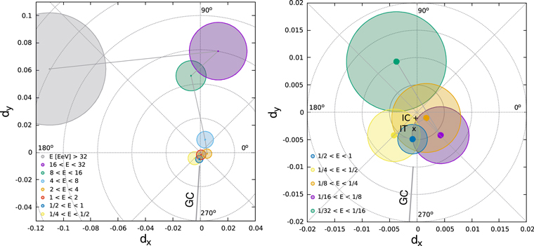
The overall behavior of the amplitudes and phases in the d_x–d_y plane is depicted in Figure 2. The left panel includes the energies above 0.25 EeV while the right panel includes those below 1 EeV. In these plots, the R.A. α_d is the polar angle, measured anticlockwise from the x-axis (so that ${d}_{x}={d}_{\perp }\cos {\alpha }_{d}$ and ${d}_{y}={d}_{\perp }\sin {\alpha }_{d}$). The circles shown have a radius equal to the 1σ uncertainties ${\sigma }_{x,y}$ in the dipole components d_x,y (reported in the Table 1), effectively including ∼39% of the two-dimensional confidence region. One can appreciate in this plot how the amplitudes decrease for decreasing energies, and how the phases change as a function of the energy, pointing almost in the opposite direction of the Galactic center above 4 EeV and not far from it below 1 EeV.

Zoom In Zoom Out Reset image size

The values of the anisotropy parameters obtained above are based, by construction, on the event content in the energy intervals under scrutiny. The finite resolution on the energies induces bin-to-bin migration of events. Due to the steepness of the energy spectrum, the migration happens especially from lower to higher energy bins. This influences the energy dependence of the recovered parameters. However, given that the size of the energy bins chosen here is much larger than the resolution, the migration of events remains small enough to avoid significant distortions for the recovered values above full efficiency. For instance, given the energy resolution of the SD1500 array (Verzi 2019) and assuming a dipole amplitude scaling as E^0.8, as was found in The Pierre Auger Collaboration (2018) to approximately hold above 4 EeV, the impact of the migrations remains below an order of magnitude smaller than the statistical uncertainties associated to the recovered parameters. In the energy range below full efficiency, additional systematic effects enter into play on the energy estimate. We note that forward-folding simulations of the response function effects into an injected anisotropy show that the recovered parameters are not impacted by more than their current statistical uncertainties. A complete unfolding of these effects is left for future studies. It requires an accurate knowledge of the response function of the SD arrays down to low energies, which is not available at the moment.

We have updated the searches for anisotropies on large angular scales using the CRs detected by the Pierre Auger Observatory. The analysis covered more than three orders of magnitude in energy, including events with $E\geqslant 0.03$ EeV and hence encompassing the expected transition between Galactic and extragalactic origins of the CRs. This was achieved by studying the first-harmonic modulation in R.A. of the CR fluxes determined with the SD1500 and the SD750 surface detector arrays. This allowed us to determine the equatorial component of a dipolar modulation, ${{\boldsymbol{d}}}_{\perp }$, or eventually to set strict upper bounds on it.

For the inclusive bin above 8 EeV, the first-harmonic modulation in R.A. leads to an equatorial dipole amplitude ${d}_{\perp }={0.060}_{-0.009}^{+0.010}$, which has a probability to arise by chance from an isotropic distribution of 1.4 × 10⁻⁹, corresponding to a two-sided Gaussian significance of 6σ. The phase of the maximum of this modulation is at α_d = 98° ± 9°, indicating an extragalactic origin for these CRs. When splitting the bin above 8 EeV, as originally done in The Pierre Auger Collaboration (2018), one finds indications of an increasing amplitude with increasing energies, and the direction of the dipole suggests that it has an extragalactic origin in all the three bins considered. A growing dipole amplitude for increasing energies could for instance be associated with the larger relative contribution to the flux that arises at high energies from nearby sources, that are more anisotropically distributed than the integrated flux from the distant ones. A suppression of the more isotropic contribution from distant sources is expected to result from the strong attenuation of the CR flux that should take place at the highest energies as a consequence of their interactions with the background radiation (Greisen 1966; Zatsepin & Kuzmin 1966).

At energies below 8 EeV, none of the amplitudes are significant, and we set 99% CL upper bounds on d_⊥ at the level of 1%–3%. The phases measured in most of the bins below 1 EeV are not far from the direction toward the Galactic center. All this suggests that the origin of these dipolar anisotropies changes from a predominantly Galactic one to an extragalactic one somewhere in the range between 1 EeV and few EeV. The small size of the dipolar amplitudes in this energy range, combined with the indications that the composition is relatively light (The Pierre Auger Collaboration 2014a), disfavor a predominant flux component of Galactic origin at $E\gt 1$ EeV (The Pierre Auger Collaboration 2013). Models of Galactic CRs relying on a mixed mass composition, with rigidity dependent spectra, have been proposed to explain the knee (at ∼4 PeV) and second-knee (at ∼0.1 EeV) features in the spectrum (Candia et al. 2003). The predicted anisotropies depend on the details of the Galactic magnetic field model considered and, below 0.5 EeV, they are consistent with the upper bounds we obtained. An extrapolation of these models, considering that there is no cutoff in the Galactic component, would predict dipolar anisotropies at the several percent level beyond the EeV, in tension with the upper bounds in this range. The conflict is even stronger for Galactic models (Calvez et al. 2010) having a light CR composition that extends up to the ankle energy (at ∼5 EeV). The presence of a more isotropic extragalactic component making a significant contribution already at EeV energies could dilute the anisotropy of Galactic origin, so as to be consistent with the bounds obtained. Note that even if the extragalactic component were completely isotropic in some reference frame, the motion of the Earth with respect to that system could give rise to a dipolar anisotropy through the Compton–Getting effect (Compton & Getting 1935). For instance, for a CR distribution that is isotropic in the CMB rest frame, the resulting Compton–Getting dipole amplitude would be about 0.6% (Kachelriess & Serpico 2006). This amplitude depends on the relative velocity and on the CR spectral slope, but not directly on the particle charge. The deflections of the extragalactic CRs caused by the Galactic magnetic field are expected to further reduce this amplitude, and also to generate higher harmonics, in a rigidity dependent way, so that the exact predictions are model dependent. The Compton–Getting extragalactic contribution to the dipolar anisotropy is hence below the upper limits obtained.

More data, as well as analyses exploiting the discrimination between the different CR mass components that will become feasible with the upgrade of the Pierre Auger Observatory currently being implemented (Castellina 2019), will be crucial to understand in depth the origin of the CRs at these energies and to learn how their anisotropies are produced.

The successful installation, commissioning, and operation of the Pierre Auger Observatory would not have been possible without the strong commitment and effort from the technical and administrative staff in Malargüe. We are very grateful to the following agencies and organizations for financial support:

Argentina—Comisión Nacional de Energía Atómica; Agencia Nacional de Promoción Científica y Tecnológica (ANPCyT); Consejo Nacional de Investigaciones Científicas y Técnicas (CONICET); Gobierno de la Provincia de Mendoza; Municipalidad de Malargüe; NDM Holdings and Valle Las Leñas; in gratitude for their continuing cooperation over land access; Australia—the Australian Research Council; Brazil—Conselho Nacional de Desenvolvimento Científico e Tecnológico (CNPq); Financiadora de Estudos e Projetos (FINEP); Fundação de Amparo à Pesquisa do Estado de Rio de Janeiro (FAPERJ); São Paulo Research Foundation (FAPESP) grants No. 2010/07359-6 and No. 1999/05404-3; Ministério da Ciência, Tecnologia, Inovações e Comunicações (MCTIC); Czech Republic—grant No. MSMT CR LTT18004, LO1305, LM2015038 and CZ.02.1.01/0.0/0.0/16 013/0001402; France—Centre de Calcul IN2P3/CNRS; Centre National de la Recherche Scientifique (CNRS); Conseil Régional Ile-de-France; Département Physique Nucléaire et Corpusculaire (PNC-IN2P3/CNRS); Département Sciences de l'Univers (SDU-INSU/CNRS); Institut Lagrange de Paris (ILP) grant No. LABEX ANR-10-LABX-63 within the Investissements d'Avenir Programme grant No. ANR-11-IDEX-0004-02; Germany—Bundesministerium für Bildung und Forschung (BMBF); Deutsche Forschungsgemeinschaft (DFG); Finanzministerium Baden-Württemberg; Helmholtz Alliance for Astroparticle Physics (HAP); Helmholtz-Gemeinschaft Deutscher Forschungszentren (HGF); Ministerium für Innovation, Wissenschaft und Forschung des Landes Nordrhein-Westfalen; Ministerium für Wissenschaft, Forschung und Kunst des Landes Baden-Württemberg; Italy—Istituto Nazionale di Fisica Nucleare (INFN); Istituto Nazionale di Astrofisica (INAF); Ministero dell'Istruzione, dell'Universitá e della Ricerca (MIUR); CETEMPS Center of Excellence; Ministero degli Affari Esteri (MAE); México—Consejo Nacional de Ciencia y Tecnología (CONACYT) No. 167733; Universidad Nacional Autónoma de México (UNAM); PAPIIT DGAPA-UNAM; The Netherlands—Ministry of Education, Culture and Science; Netherlands Organisation for Scientific Research (NWO); Dutch national e-infrastructure with the support of SURF Cooperative; Poland -Ministry of Science and Higher Education, grant No. DIR/WK/2018/11; National Science Centre, grants No. 2013/08/M/ST9/00322, No. 2016/23/B/ST9/01635 and No. HARMONIA 5–2013/10/M/ST9/00062, UMO-2016/22/M/ST9/00198; Portugal—Portuguese national funds and FEDER funds within Programa Operacional Factores de Competitividade through Fundação para a Ciência e a Tecnologia (COMPETE); Romania—Romanian Ministry of Research and Innovation CNCS/CCCDI-UESFISCDI, projects PN-III-P1-1.2-PCCDI-2017-0839/19PCCDI/2018 and PN18090102 within PNCDI III; Slovenia—Slovenian Research Agency, grants P1-0031, P1-0385, I0-0033, N1-0111; Spain—Ministerio de Economía, Industria y Competitividad (FPA2017-85114-P and FPA2017-85197-P), Xunta de Galicia (ED431C 2017/07), Junta de Andalucía (SOMM17/6104/UGR), Feder Funds, RENATA Red Nacional Temática de Astropartículas (FPA2015-68783-REDT) and María de Maeztu Unit of Excellence (MDM-2016-0692); USA—Department of Energy, Contracts No. DE-AC02-07CH11359, No. DE-FR02-04ER41300, No. DE-FG02-99ER41107 and No. DE-SC0011689; National Science Foundation, grant No. 0450696; The Grainger Foundation; Marie Curie-IRSES/EPLANET; European Particle Physics Latin American Network; and UNESCO.

In Table 2 we report the amplitudes and probabilities obtained with the SD1500 array at the solar and antisidereal frequencies, in all bins above 2 EeV for which the Rayleigh analysis was applied at the sidereal frequency. One can see that all these amplitudes are consistent with being fluctuations, showing then no signs of remaining systematic effects. We also report in Table 3 the equatorial dipole amplitudes and phases obtained with the east–west method above 2 EeV, and compare them with the results for the same data sets that were obtained with the Rayleigh method (reported in Table 1). The inferred equatorial dipole amplitudes turn out to be consistent, although the statistical uncertainty obtained with the east–west method is larger by a factor $\pi \langle \cos \delta \rangle /2\langle \sin \theta \rangle$ (Bonino et al. 2011). Given that above full trigger efficiency one has that $\langle \sin \theta \rangle \simeq 0.58$ when considering θ < 60°, as we do for E < 4 EeV, or $\langle \sin \theta \rangle \simeq 0.65$ when considering θ < 80°, as we do for E ≥ 4 EeV, and that $\langle \cos \delta \rangle \simeq 0.78$ in both zenith ranges, the statistical uncertainties obtained in the east–west analysis are larger by a factor of about 2.1 than those obtained with the Rayleigh analysis for θ < 60°, or by a factor of about 1.9 for θ < 80°, as can be seen in Table 3.

Table 2.  Fourier Amplitudes at the Solar and Antisidereal Frequencies, and the Probabilities to Get Larger Values from Statistical Fluctuations of an Isotropic Distribution, for the Different Energy Bins above 2 EeV

E (EeV)	N	Solar		Antisidereal
		r (%)	$P(\geqslant r)$	r (%)	$P(\geqslant r)$
2–4	283,074	${0.6}_{-0.2}^{+0.3}$	0.07	${0.5}_{-0.2}^{+0.3}$	0.20
4–8	88,325	${0.8}_{-0.3}^{+0.5}$	0.24	${0.5}_{-0.2}^{+0.5}$	0.59
8–16	27,271	${0.6}_{-0.2}^{+1.1}$	0.79	${0.5}_{-0.1}^{+1.1}$	0.83
16–32	7664	${1.1}_{-0.3}^{+2.0}$	0.79	${3.1}_{-1.1}^{+1.9}$	0.16
≥32	1993	${1.5}_{-0.1}^{+4.4}$	0.90	${1.3}_{-0.0}^{+4.6}$	0.92
≥8	36,928	${0.3}_{-0.0}^{+1.1}$	0.93	${1.0}_{-0.4}^{+0.8}$	0.39

Download table as:  ASCIITypeset image

Table 3.  Equatorial Dipole Reconstruction above 2 EeV Obtained Using the East–West Method

		East–West (SD1500)				Rayleigh (SD1500)
E (EeV)	N	${d}_{\perp }$ (%)	${\sigma }_{x,y}$ (%)	${\alpha }_{d}\ (^\circ )$	$P(\geqslant {d}_{\perp })$	${d}_{\perp }$ (%)	${\sigma }_{x,y}$ (%)	${\alpha }_{d}\ (^\circ )$
2–4	283,074	${0.2}_{-0.2}^{+0.9}$	0.72	−16 ± 167	0.94	${0.5}_{-0.2}^{+0.4}$	0.34	−11 ± 55
4–8	88,325	${1.7}_{-0.7}^{+1.3}$	1.1	41 ± 38	0.33	${1.0}_{-0.4}^{+0.7}$	0.61	69 ± 46
8–16	27,271	${6.4}_{-1.7}^{+2.3}$	2.1	147 ± 18	$8.3\times {10}^{-3}$	${5.6}_{-1.0}^{+1.2}$	1.1	97 ± 12
16–32	7664	${9.3}_{-3.0}^{+4.5}$	3.9	67 ± 24	$5.8\times {10}^{-2}$	${7.5}_{-1.8}^{+2.3}$	2.1	80 ± 17
≥32	1993	${25}_{-6}^{+9}$	7.6	151 ± 17	$4.1\times {10}^{-3}$	${13}_{-3}^{+5}$	4.1	152 ± 19
≥8	36,928	${6.6}_{-1.5}^{+2.0}$	1.8	132 ± 15	$8.6\times {10}^{-4}$	${6.0}_{-0.9}^{+1.0}$	0.94	98 ± 9

Note. Indicated are the number of events, amplitude of ${d}_{\perp }$, uncertainty ${\sigma }_{x,y}=\sigma /\langle \cos \delta \rangle$ of the components d_x or d_y, R.A. phase ${\alpha }_{d}$ and probability $P(\geqslant {d}_{\perp })$ to get a larger amplitude from fluctuations of an isotropic distribution. For comparison we also include in the last two columns the values of ${d}_{\perp }$ and ${\alpha }_{d}$ that were obtained in the Rayleigh analysis (reported in Table 1).

Download table as:  ASCIITypeset image