


Abstract
This study presents results from continuous measurements of stem CO2 efflux carried out for seven growing seasons in a young Norway spruce forest. The objective of the study was to determine differences in temperature sensitivity of stem CO2 efflux (Q10) during night (when sap flow is zero or nearly zero), during early afternoon (when the maximum rate of sap flow occurs) and during two transition periods between the aforementioned periods. The highest Q10 was recorded during the period of zero sap flow, while the lowest Q10 was observed in period of the highest sap flow. Calculating Q10 using only data from the period of zero sap flow resulted in a Q10 that was higher by as much as 19% compared with Q10 calculated using 24 h data. On the other hand, basing the calculation on data from the period of the highest sap flow yielded 5.6% lower Q10 than if 24 h data were used. Considering that change in CO2 efflux lagged in time behind changing stem temperature, there was only a small effect on calculated Q10 for periods with zero and the highest sap flow. A larger effect of the time lag (by as much as 15%) was observed for the two transition periods. Stem CO2 efflux was modelled based on the night CO2 efflux response to temperature. This model had a tendency to overestimate CO2 efflux during daytime, thus indicating potential daytime depression of stem CO2 efflux compared with the values predicated on the basis of temperature caused by CO2 transport upward in the sap flow. This view was supported by our results inasmuch as the overestimation grew with sap flow that was modelled on the basis of photosynthetically active radiation and vapour pressure deficit.
Introduction
Stem respiration is an important component of an ecosystem carbon budget. It usually accounts for about 7–25% of total ecosystem respiration of mature forest ecosystems (Bolstad et al. 2004, Zha et al. 2004, 2007, Acosta et al. 2008, Tang et al. 2008, Khomik et al. 2010).
Stem respiration takes place within living cells of the inner bark, cambium and xylem (Teskey et al. 2008). It provides energy for such maintenance processes of the existing cells as, for example, turnover of proteins, nutrient uptake and ion fluxes (and thus is termed maintenance respiration; Penning de Vries 1975, Amthor 1989). During cambial reactivation and stem growth, a tree has extra respiratory requirements from activated dividing cells and their consequent differentiation (termed growth respiration; Ryan 1990, Amthor 2000, Gruber et al. 2009).
A dominant environmental driver of stem respiration is temperature (Stockfors 2000, Zha et al. 2004, Saveyn et al. 2008), which is often used to predict stem respiration (Stockfors 2000, Acosta et al. 2008, Holtta and Kolari 2009). At the biochemical level, temperature sensitivity of respiration (Q10) is generally assumed to be around 2 (Atkin et al. 2002, Davidson et al. 2006). However, studies like those by Tjoelker et al. (2001), Atkin and Tjoelker (2003) and Atkin et al. (2005) show Q10 variability with temperature due to thermal acclimation of respiration. Stem respiration is often estimated as CO2 efflux from the stem surface but its Q10 can differ from that of respiration because of internal CO2 fluxes.
A substantial part of CO2 diffuses directly out of the stem into the atmosphere, which is given by the great CO2 concentration gradient between stem and atmosphere (Holtta and Kolari 2009). A part can, however, be dissolved in sap and transported upward by the transpiration stream (Negisi 1979, Gansert and Burgdorf 2005, Teskey and McGuire 2007, Salomon et al. 2016). A small amount of CO2 is stored within the stem and can be observed as changes in CO2 concentration (Teskey and McGuire 2007, Salomon et al. 2016). Therefore, measured CO2 efflux from the stem surface is a result mainly of these processes (Trumbore et al. 2013). Studies from McGuire and Teskey (2004), Teskey and McGuire (2007) and Salomon et al. (2016) have described CO2 diffusion into the atmosphere to be the largest component of locally respired CO2. The proportion of CO2 transported in xylem sap has been found to be as much as 55% (McGuire and Teskey 2004, Bowman et al. 2005, Saveyn et al. 2008, Angert et al. 2012). Teskey and McGuire (2007) described the diurnal dynamics of this component of CO2 flux within the stem, which was characterized by low values through nighttime but with a substantial increase during daytime, when the transpiration stream is induced. This finding is consistent with the results of Negisi (1979), Gansert and Burgdorf (2005), Saveyn et al. (2008), Buzkova et al. (2015) and Salomon et al. (2016), who observed lower measured CO2 efflux during midday than expected from temperature.
A number of studies have observed a varying relationship between stem CO2 efflux and temperature over the year (Stockfors and Linder 1998, Maier 2001, Zha et al. 2004, Acosta et al. 2008, Darenova et al. 2018). The relationship between stem and temperature can also be altered on a diurnal basis when CO2 transport in the xylem sap causes CO2 efflux lower than expected from temperature (Negisi 1979). Measurements from different sub-daily periods can produce different results, and that can make it difficult to compare studies that are otherwise generally similar. It also affects models of forest carbon balance.
The present study is based on continuous measurements of stem CO2 efflux and temperature and focuses on how diurnal internal stem CO2 fluxes can affect Q10 estimation. Q10 was determined during nighttime, when there is zero sap flow; early afternoon, when the sap flow rate is at its highest; and two transition periods (one characterized by increasing and the other by decreasing transpiration). Also examined is whether the differences among the sub-daily periods are constant throughout the growing season. The study also analysed whether there is any effect due to a time lag in stem CO2 efflux behind stem temperature on calculated Q10 and when that potential effect is its greatest. We proceeded on the assumption that during nighttime, when no CO2 is transported by the transpiration stream, the direct CO2 diffusion into the atmosphere is at its highest, and therefore we considered that temperature effect on CO2 efflux is not disturbed at that time by other factors. Therefore, the relationship between temperature and stem CO2 efflux from the period was used to model CO2 efflux and to search for drivers resulting in differences between measured and modelled stem CO2 efflux.
Materials and methods
Study site
The experimental Norway spruce (Picea abies [L.] Karst) forest stand is situated at the Experimental Ecological Study Site at Bílý Kříž (49°30′ N, 18°32′ E, 875 m above sea level) located within the Moravian–Silesian Beskydy Mountains in the Czech Republic. The 6 ha forest stand was planted in 1981 using 4-year-old seedlings on a 12.5° slope with a south–southwest exposure. Main characteristics of the forest stand over the experimental period are summarized in Table 1. Reduction in tree density and leaf area index in 2006 and 2012 resulted from fallen trees during preceding winters. The site is characterized by mean annual temperature of 6.8 °C and mean annual total precipitation of 1280 mm. The soil is a predominantly Haplic Podzol (FAO soil classification system).
Characteristics of the experimental forest stand for individual studied years, mean stem temperature, sum of precipitation and number of rainy days, for the period between 1 May and 31 October 2005–13.
| 2005 | 2006 | 2007 | 2008 | 2009 | 2010 | 2011 | 2012 | 2013 | |
|---|---|---|---|---|---|---|---|---|---|
| Tree density (trees ha−1) | 1664 | 1580 | 1508 | 1500 | 1492 | 1488 | 1488 | 1268 | 1256 |
| Mean tree height (m) | 11.2 | 11.7 | 12.2 | 12.5 | 13.1 | 13.6 | 14.3 | 14.8 | 15.3 |
| Stem diameter at breast height (cm) | 13.3 | 14.0 | 14.6 | 15.3 | 15.9 | 16.4 | 16.9 | 17.9 | 18.2 |
| Leaf area index | 11.8 | 8.0 | 8.5 | 9.5 | 9.6 | 10.1 | 10.2 | 7.5 | 7.7 |
| Mean stem temperature (°C) | 12.1 | 13.5 | 12.8 | 12.3 | 12.2 | 11.6 | 12.7 | 12.2 | 12.6 |
| Precipitation (mm) | 854 | 794 | 896 | 688 | 618 | 1187 | 665 | 580 | 586 |
| Number of rainy days | 94 | 80 | 91 | 80 | 97 | 109 | 93 | 88 | 88 |
Sap flow measurement
Sap flow determined in the stem segment characterizes the transpiration stream through the tree. Sap flow was measured ~1.3 m above the ground on eight trees having diameter at breast height ranging from 13.6 to 26.4 cm. Measurements were conducted from June to October 2016. There were no sap flow measurements during the period of stem CO2 efflux measurements. However, we expect no substantial differences in diel dynamics of sap flow between these two periods.
For the sap flow measurements, the tissue heat balance method (Čermák et al. 2004) was applied using EMS 51 sensors (EMS, Brno, Czech Republic). The sap flow system consisted of the controlling module connected to the measuring points composed of four stainless steel electrodes and needle temperature sensors. Tree conductive xylem tissue around three flat stainless electrodes was supplied with electric power in order to heat the water and to maintain a constant temperature difference (set at 2 °C) between the three heated electrodes and a fourth reference (non-heated) electrode. The mass of water passing through the measuring points in the stem was automatically calculated from the electrical power used to raise the temperature of water passing through the heated space. Measurement was conducted once each minute and mean data values were calculated and recorded in 10-min intervals. The output value was calculated in terms of sap flow per one centimetre of trunk circumference (kg H2O h–1 or day–1, per cm), (Kučera 2010). Based upon a baseline created from the nighttime zero values in the situation of no evaporation demand, the original data were processed in Mini32 software (Mini32 ver. 10.02.02, EMS) to eliminate the heat dissipation loss from the sap flow value. These sap flow data from 2016 were used to assess diurnal courses of sap flow and to model sap flow for the years when stem CO2 efflux was measured (see next section).
Stem CO2 efflux measurement
CO2 efflux measurements were carried out for the period between 1 May and 31 October 2005–13. Eight experimental trees were selected in an area of 30 m2 within the forest. Stem diameter at breast height of the trees ranged between 12 and 21 cm in 2005 and between 13 and 25 cm in 2013. On these, CO2 efflux from the stem surface (EA) was measured using an automated, closed dynamic (non-steady-state, through-flow) system (Darenova et al. 2018). The system consisted of eight chambers (Figure 2 in Darenova et al. 2018) and control units for chamber closing, an infrared gas analyser (Li-840, LI-COR, Lincoln, NE, USA), and a personal computer with control software and additional analogue input and digital output hardware. The chambers consisted of a frame and a chamber head. The frames were of a rectangular shape with inner dimensions 5.5 × 11.0 cm and made of duralumin. They were affixed to the tree trunk by belts at breast height from the northern side (due to the forest stand’s sun exposure and to avoid direct sun radiation on the chamber) and provided with neoprene sealing from both sides, adjacent to the tree trunk and to the chamber. The chamber heads were made of stainless steel and had a half-cylinder shape with 12 cm height and 6.5 cm diameter. They were attached to an arm affixed to the tree trunk by two belts above the frames and which enabled closing the chamber head over the frame using a pneumatic piston and compressed air.
Additional measurements
Stem temperature was measured continuously at the same time as stem CO2 efflux using thermometers (PT 100, Sensit, Roznov pod Radhostem, Czech Republic) permanently installed ~5 cm below the chambers in the cambium layer. The bark was carefully cut in an L-shape and the thermometer was inserted just below the bark. The bark and the thermometer were then fixed by a sticking tape.
Data analyses
We calculated mean seasonal (June–October) sap flow for each hour of the day and of these results the 24 h period was divided into four shorter sub-daily periods: 0:00–6:00 h, characterized by zero sap flow; 6:00–11:00 h, a morning transition period with increasing sap flow rate; 11:00–17:00 h, the time of the highest sap flow; and 17:00–24:00 h, an evening transition period with decreasing sap flow rate. First we selected the 6-h period for the nighttime and then the midday 6-h period with high sap flow, but kept the morning transition period 5-h long to be sure we had three EA values for each day.
The individual seasons were divided into seven periods on the basis of stem growth rate as done in the study by Darenova et al. (2018): pI (1–22 May, gradual acceleration of stem growth), pII (23 May–11 June, rapid stem growth increment dynamic), pIII (12 June–8 July, culmination of the stem growth dynamic), pIV (9–28 July, slight decline of the stem growth), pV (29 July–23 August, drop of stem growth dynamic), pVI (24 August–28 September, deceleration of stem growth dynamic) and pVII (29 September–31 October, termination of stem growth).
The parameters of the exponential temperature function of EA, Q10 and R10 (CO2 efflux at a temperature of 10 °C) were determined for the period of zero sap flow separately for individual seasonal periods. These parameters were used to model stem CO2 efflux on the basis of continuous stem temperature measurements.
Residuals between the measured vs modelled CO2 effluxes (Eq. (5)) were compared with modelled sap flow.
The time lag between stem temperature and EA was estimated at each chamber position for all seasonal periods of each year. Stem temperature observations were shifted in time up to 8 h and fitted (Eq. (3)) against EA measurements. The time lag was determined and the time shift in stem temperature that led to the highest R2 for the relationship between the EA and stem temperature.
Statistical analyses were performed using SigmaPlot 11.0 analytical software (Systat Software, San Jose, CA, USA). Differences in Q10 between individual sub-daily periods were tested by one-way ANOVA. Statistical significance of all analyses was tested at probability level α = 0.05.
Results
Sap flow
Daily sap flow maxima in 2016 ranged between 0.000 and 0.039 kg h–1 per cm of the tree circumference with maxima in June. On the diurnal scale, the lowest sap flow was observed during nighttime when between 0:00 and 6:00 h it was zero or very close to zero. The highest sap flow rates, meanwhile, were measured between 13:00 and 15:00 h. Based upon these results, the day was divided into four sub-daily periods (Figure 1).
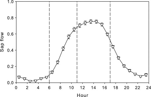
Mean diurnal courses of sap flow for the period between May and October 2016. Values are normalized by the respective daily maximum. One-hourly means ± SE are given. Vertical dashed lines show dividing of the day into four sub-daily periods on the basis of sap flow rate.
The R2 of this regression reached a value of 0.87. This equation was used to model sap flow for the period of stem CO2 efflux measurement.
Diurnal variability of Q10
The seasonal variability of stem CO2 efflux was driven by stem temperature. The relationship between stem temperature and EA was characterized by R2 of the exponential regression ranging mostly between 0.7 and 0.9 (P < 0.0001). Q10 calculated from 24 h data ranged between 2.30 and 2.94, with the lowest values in seasonal periods pIV and pV. The same pattern was observed for Q10 calculated separately for each sub-daily period (Figure 2A). The highest Q10 was reached for the period of zero sap flow, while the lowest Q10 was found during the period of the highest sap flow. Calculating Q10 using data only from the zero sap flow period resulted in a Q10 that was higher by as much as 19% compared with Q10 calculated from all 24 h data. On the other hand, basing the calculation on data from the period of zero sap flow yielded 5.6% lower Q10 than if 24 h data were used (Figure 2B). Both transient periods showed higher Q10 compared with the 24 h period but not so much as did the period of zero sap flow. Differences between periods with zero and the highest sap flow were statistically significant through the season. The significance of the differences between other pairs of sub-daily periods was variable over the season.
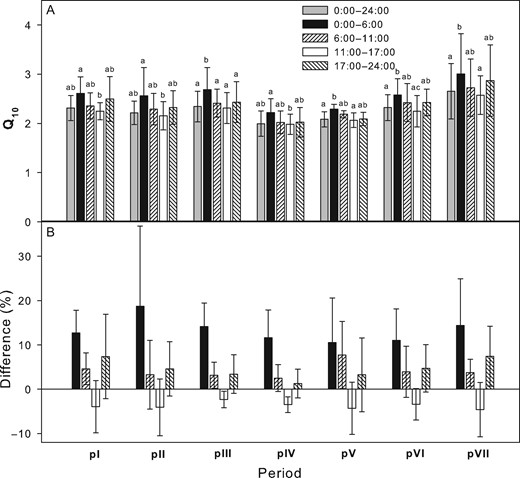
(A) Mean Q10 calculated for different sub-daily and seasonal periods (pI–pVI) that correspond with stem growth (pI: 1–22 May, pII: 23 May–8 July, pIII: 12 June–8 July, pIV: 9–28 July, pV: 29 July–23 August, pVI: 24 August–28 September and pVII: 29 September–31 October). (B) Percentage differences of Q10 calculated for individual day periods and Q10 calculated for the 24 h periods. Error bars represent SD. Lowercase letters indicate statistically significant differences among the stands on the same measurement date (P < 0.05).
Effect of EA time lag on Q10
The closest relationship between stem temperature and EA was found for the temperature 2 h before stem CO2 efflux measurements. This time lag was consistent through all seasonal periods (pI–pVII) in all years.
Considering the time lag in EA behind stem temperature had only a small effect on Q10 calculated for the 24 h period. The change amounted to just a few percentage points. Among the individual sub-daily periods, the smallest changes in Q10 caused by the time lag were observed for the periods with zero and the highest sap flow (Figure 3). The changes did not exceed 5%. These two periods also correspond to times when stem temperature changes are small (Figure 1).
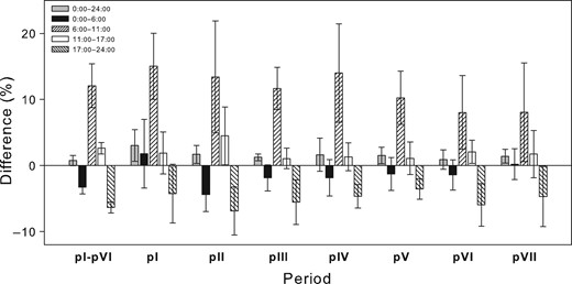
Percentage differences of Q10 calculated with stem CO2 efflux time lag of 2 h behind stem temperature from Q10 calculated with no time lag for five sub-daily periods (0:00–24:00, 0:00–6:00, 6:00–11:00, 11:00–17:00 and 17:00–24:00 h). Seasonal periods labelled as pI–pVI correspond with stem growth (pI: 1–22 May, pII: 23 May–8 July, pIII: 12 June–8 July, pIV: 9–28 July, pV: 29 July–23 August, pVI: 24 August–28 September and pVII: 29 September–31 October). Error bars represent SD.
A greater effect of the time lag was observed during the transient periods. The morning transient period showed the biggest changes, as Q10 rose by as much as 15% after implementing time lag into the calculation. During the evening transient period, calculation with the time lag resulted in Q10 lower mostly by about 5%.
Dynamics of daytime depression of EA compared with Em
CO2 efflux was modelled (Em) on the basis of parameters Q10 and R10 calculated for the period of zero sap flow, which are summarized in Table 2. Small residuals were found for the period of zero sap flow, the mean difference being 0.01 μmol m−2s−1 (Figure 4). On the contrary, this approach resulted in Em being higher compared with EA during daytime. The greatest Em residua from EA were observed for the period of the highest sap flow. This period was also characterized by a large number of upper outliers (as indicated by the dimensions of the box and error bars) and substantially higher mean compared with median. The variability of the differences between Em and EA did not correspond to changes in daily sap flow for the zero sap flow period. For daytime, however, and particularly for the period of the highest sap flow, the magnitude of the residuals increased with daily sap flow in all years (Figure 5). The relationship between the differences in EA and Em and daily sap flow was characterized best by the exponential regression having R2 between 0.1 and 0.84. The regressions were statistically significant in all years (P = 0.0002 for 2005 and P < 0.0001 for other years) and their parameters are summarized in Table 3. The greatest differences between Em and EA and their steepest increase with daily sap flow occurred in 2013.
Parameters Q10 and R10 of the exponential function of the relationship between stem CO2 efflux and stem temperature during nighttime. Seasonal periods labelled as pI–pVI correspond to stem growth.
| pI | pII | pIII | pIV | pV | pVI | pVII | ||
|---|---|---|---|---|---|---|---|---|
| 2005 | Q10 | 2.18 | 2.40 | 2.73 | 2.73 | 2.98 | 2.78 | 2.05 |
| R10 | 0.93 | 0.76 | 0.76 | 0.75 | 0.66 | 0.59 | 0.74 | |
| 2006 | Q10 | 1.58 | 2.21 | 2.43 | 2.76 | 2.54 | 2.83 | 3.51 |
| R10 | 0.92 | 0.89 | 1.16 | 0.92 | 0.85 | 0.87 | 0.91 | |
| 2007 | Q10 | 2.47 | 1.92 | 2.73 | 2.99 | 3.13 | 2.68 | 2.34 |
| R10 | 1.55 | 1.64 | 1.30 | 1.30 | 1.12 | 1.26 | 1.37 | |
| 2008 | Q10 | 2.32 | 1.87 | 2.19 | 2.68 | 2.39 | 2.28 | 1.94 |
| R10 | 1.74 | 1.59 | 1.24 | 1.52 | 1.21 | 1.49 | 1.88 | |
| 2010 | Q10 | 2.25 | 2.33 | 2.29 | 2.28 | 2.10 | 2.14 | 2.44 |
| R10 | 1.67 | 0.92 | 1.04 | 1.43 | 1.14 | 1.53 | 1.21 | |
| 2011 | Q10 | 2.67 | 1.94 | 2.35 | 2.85 | 2.55 | 2.77 | 2.76 |
| R10 | 1.33 | 0.84 | 0.81 | 1.15 | 1.19 | 0.92 | 1.18 | |
| 2013 | Q10 | 3.12 | 2.33 | 3.76 | 3.37 | 3.86 | 2.54 | 2.30 |
| R10 | 1.26 | 0.55 | 0.67 | 0.76 | 0.90 | 0.63 | 0.70 |
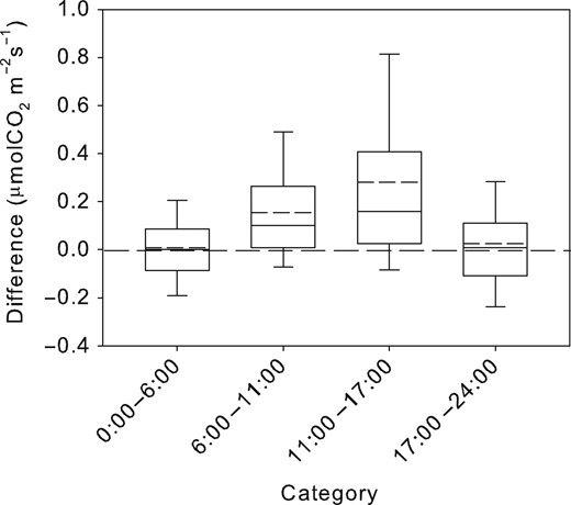
Difference of the measured from modelled stem CO2 efflux for four different sub-daily periods (0:00–6:00 h, period with zero sap; 6:00–11:00 h, morning transition period; 11:00–17:00 h, period with the highest sap flow; and 17:00–24:00 h, evening transition period). Solid lines in the boxes show medians while dashed lines indicate means. The boundaries of the boxes indicate the 25th and 75th percentiles, and the error bars indicate 10th and 90th percentiles.
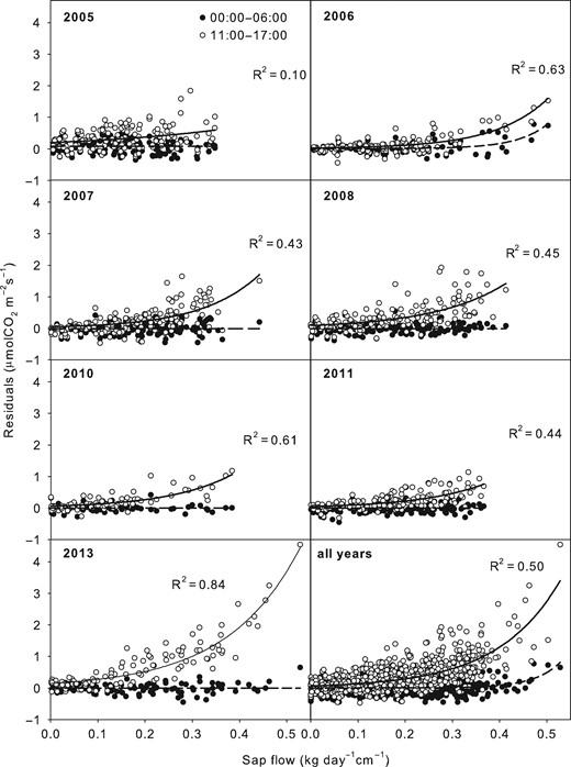
Relationships between residuals of measured vs modelled CO2 effluxes and mean sum of sap flow for two sub-daily periods (0:00–6:00 h, period with zero sap and 11:00–17:00 h, period with the highest sap flow). R2 values characterize the exponential functions. Other characteristics of these functions are summarized in Table 3.
Parameters, F- and P-values of exponential regressions () for the relationships between differences of measured vs modelled stem CO2 effluxes and daily sum sap flow (kg cm−1) during the period between 11:00 and 17:00 h.
| a | b | R2 | F | P | |
|---|---|---|---|---|---|
| 2005 | 0.1982 | 3.1480 | 0.09 | 15.1 | 0.0002 |
| 2006 | 0.0178 | 8.9394 | 0.63 | 217.6 | <0.0001 |
| 2007 | 0.0455 | 8.1958 | 0.41 | 111.8 | <0.0001 |
| 2008 | 0.0909 | 6.6538 | 0.45 | 144.1 | <0.0001 |
| 2010 | 0.0601 | 7.4873 | 0.61 | 145.4 | <0.0001 |
| 2011 | 0.0528 | 7.2768 | 0.44 | 130.6 | <0.0001 |
| 2013 | 0.1422 | 6.5157 | 0.84 | 620.1 | <0.0001 |
| All | 0.0642 | 7.5137 | 0.50 | 992.4 | <0.0001 |
Discussion
Diurnal variability of Q10
An accurate understanding of respiration’s response to temperature is critical for estimating global carbon balance and its response to current climate change. Q10 in our study ranged between 1.42 and 4.56 depending on year and seasonal or sub-daily period. These results were mostly within the range between 1.5 and 3.0 reported in other studies for different species (Stockfors and Linder 1998, Kim et al. 2007, Zha et al. 2007, Acosta et al. 2008, Rodriguez-Calcerrada et al. 2014). Although Q10 around 4 is rare, Brito et al. (2010) did observe Q10 between 3.0 and 4.4 for Pinus trees during a warm and dry period. We observed such high Q10 just in a few cases during the post-growth period. Seasonality of Q10 has been reported in previous studies and attributed to the seasonality of growth respiration’s contribution to total stem respiration (Adu-Bredu et al. 1997, Lavigne et al. 2004) or to decrease in Q10 with rising temperature as a result of thermal acclimation of respiration and substrate limitations at high temperature (Atkin and Tjoelker 2003). This issue was discussed in detail in the previous study of Darenova et al. (2018). The authors furthermore showed that calculating Q10 for the whole growing season can result in great overestimation of Q10.
The results of this study show that in addition to this Q10 seasonality, Q10 variability should also be considered at the diel scale because Q10 differed for different sub-daily periods. The highest values were observed during the period of zero sap flow and the lowest during the period of the highest sap flow. The effect of day and night on Q10 was also analysed by Saveyn et al. (2008). They found an inconsistent effect of sub-daily period on Q10. On the other hand, Lavigne (1987) and Yang et al. (2014) had findings similar to ours. The former study reported Q10 higher in the afternoon than in the morning, and the latter observed the highest Q10 shortly after midnight and lowest in early afternoon.
According to previous studies, midday CO2 efflux can be depressed compared with that expected on the basis of temperature (Negisi 1979, Lavigne 1987, Gansert and Burgdorf 2005, Saveyn et al. 2007, 2008, Tarvainen et al. 2014, Salomon et al. 2016). This depression is usually attributed to several things: (i) decline in temperature sensitivity of EA rates with short-term increases in temperature (Tjoelker et al. 2001); (ii) midday depression of photosynthesis, and particularly during hot summer days, which provides substrate for respiration of living cells (Yang et al. 2014); (iii) refixation of respired CO2 by corticular photosynthesis (Sprugel and Benecke 1991), which we did not consider in our study because thick bark prevents light penetration in grown trees (Pfanz and Aschan 2001); (iv) loss of turgor pressure in the living stem tissues during daytime (Saveyn et al. 2007, Salomon et al. 2018); and (v) dissolving of a part of respired CO2 in xylem sap and its transport upwards in the transpiration stream as stated for example by Negisi (1979) for Pinus densiflora or by Gansert and Burgdorf (2005) for Betula pendula. The last explanation has been supported by broad research based on the mass balance approach (McGuire and Teskey 2004). Studies like those of McGuire and Teskey (2004) on Platanus occidentalis, Liquidambar styraciflua and Fagus grandifolia, Teskey and McGuire (2007) on Platanus occidentalis and Salomon et al. (2016) on Quercus pyrenaica have demonstrated the diurnal dynamics and proportions of individual components of CO2 fluxes in the stem. McGuire and Teskey (2004) stated transport flux to be the most varying component of stem respiration, with it being close to zero at night and within a wide range reaching as high as 71% during daytime. Furthermore, Teskey and McGuire (2007) observed that the transport flux may exceed CO2 efflux into the atmosphere during midday, and Salomon et al. (2016) reported the transport flux reaching a maximum 25% of stem respiration.
Effect of EA time lag on Q10
We found that integrating the EA time lag behind stem temperature affected the Q10 calculation. Incorporating time lag into Q10 calculation gives us more accurate results about the response of CO2 production to temperature changes. The time lag in our study amounted to a constant 2 h through all seasons. According to other authors, the time lag can range from 0 to 5 h (Ryan et al. 1995, Lavigne et al. 1996, Stockfors and Linder 1998, Acosta et al. 2008, Etzold et al. 2013, Tarvainen et al. 2014) and this is explained by two things: (i) measurement of stem temperature at just one place is not representative for the temperature of the entire respiring woody tissue profile (Stockfors 2000); and (ii) there is a delay between CO2 production in the living cells and CO2 efflux from the stem surface because of the strong diffusive resistance of the cambium and the bark (Eklund and Lavigne 1995, Holtta and Kolari 2009). When analysing the relationship between stem CO2 efflux and stem temperature from 2 h earlier, the parameter Q10 was substantially lower than that calculated from actual temperature for the morning transition period while for the evening transition period it was higher. On the contrary, only a small effect on Q10 was observed during periods with zero and the highest sap flow. We consider the reason for this pattern to be that there are much greater and more rapid changes of temperature during both transition periods compared with the other two periods.
The smallest effect of time lag inclusion into Q10 calculation was found for the 24 h periods, which indicates that during this period all divergences diminished and we may assume this Q10 to be the most accurate.
Dynamics of daytime depression of EA compared with Em
As discussed above, most factors attributed to causing the midday depression of EA compared with efflux expected from temperature are associated with xylem sap. The effect of water status and flux on stem CO2 efflux was reflected also in our study. EA modelled using EA temperature responses determined during the night (Em) tended to overestimate stem CO2 efflux during the days with high sap flow. As the modelled sap flow was a function of PAR and VPD, the model overestimated the CO2 efflux during warm and dry days.
Beside sap flow, decline in cell turgor during day has been reported as the reason for lower measured EA compared with that estimated on the basis of temperature (Saveyn et al. 2007). Salomon et al. (2018) concluded that cell turgor pressure is a reliable predictor of stem CO2 efflux as they observed a significant relationship between turgor pressure and the difference between CO2 efflux measured after reducing or stopping transpiration stream on one hand, and CO2 efflux modelled using EA temperature responses determined during a control period with unaffected transpiration stream on the other. Cell turgor and CO2 transport in the sap are both driven by the transpiration stream; therefore, as argued by Saveyn et al. (2007), it may be methodically challenging to separate their effects.
The two above-mentioned studies (Saveyn et al. 2007, Salomon et al. 2018) were, however, done on young trees (3-year-old). Such young trees have still limited sapwood area, sap flow is low and cell turgor loss may have more importance. The contribution of CO2 flux in sap into EA, however, increases with stem diameter (Fan et al. 2017). Therefore, we assume that the effect of sap flow during daytime on the EA residuals is much more relevant that cell turgor changes. The low turgor may have become evident in the season 2013 when the relationship between residuals between the measured vs modelled CO2 effluxes were steepest. This year was characterized by a very dry summer. As reported in Darenova et al. (2018), total precipitation in July and August was only 92 mm, which was by far the least precipitation among all the experimental years. In the other years, the July and August totals ranged between 232 and 459 mm. Although lack of water affects stem respiration generally, we may expect that during nighttime, when the stomata are closed and water loss through transpiration ceases, the tree draws water from the soil and refills its stem tissues (Čermák et al. 2015). In conditions of water stress, the transpiration stream decreases during midday and afternoon despite rising evaporation demand, because the tree cannot uptake water due to the unavailability of soil water (Čermák et al. 2015). Insufficient water supply from roots may cause stem tissues to become dehydrated, and this is reflected also in reduced respiration activity.
Recommendation for stem CO2 efflux measurements
The best option to obtain the diurnal and seasonal courses of EA is to have automated systems for continual measurements. However, such systems cannot be applied everywhere for many reasons (lack of power supply, site accessibility, high costs, etc.). Therefore, there is a question of how to get enough information to get the most accurate estimates of EA.
For analyses of longer periods (from days to year), when diurnal dynamic of EA is not relevant, EA and its temperature dependence should be determined for such periods when we can expect more or less the same wood status, such as increment rate (Darenova et al. 2018). Q10 calculated from 24 h measurements seems to best characterize EA response to temperature as it includes, to some extent, also the daytime reduction of EA.
Q10 calculated for morning and evening transition periods and for the period with the highest sap flow were closer to 24 h Q10 compared with the zero sap flow period. The absolute difference of 24 h Q10 and Q10 of the three periods was similar, but in the morning transition period the least extremes occurred. If we consider from the Figure 2B a gradual decrease of the Q10 difference from the morning transition period (6:00–11:00 h) towards the period with the highest sap flow (11:00–17:00 h), we assume that measurements in late morning can result in Q10 with residua from 24 h Q10 around 0. We consider that such Q10 values and mean daily temperature for seasonal courses or mean temperature of the corresponding period for total CO2 efflux calculation would be sufficient. At sites with meteorological measurements it is also possible to measure EA during days with very high or, on contrary low PAR and VPD, which drive sap flow. This would help to discover how EA during daytime behaves under these ‘extreme’ conditions.
For some analyses, diurnal course of stem CO2 efflux can be required, for example, to determine daytime ratio of ecosystem photosynthesis and respiration (Sun et al. 2014). This would need more measurements and analyses. We consider that measurements would include the continuous sap flow or meteorological measurement and more EA measurements under different meteorological conditions should be taken. These extended EA measurements should focus mainly on days with different sap flow. As the residua of measured EA and EA modelled from stem temperature increase with sap flow, these measurements should be focused on clear and dry days (with high PAR and VPD).
To get the right timing of minima and maxima of modelled EA, time lag of EA behind temperature should be included in EA modelling. Accurate determination of the time lag requires intensive 24 h measurement to get the whole diurnal course and see and determine the hysteresis between stem CO2 efflux and stem temperature (Yang et al. 2014). It should be also checked whether this is constant or variable through year.
Conclusions
In this study, we found variable temperature response of stem CO2 efflux (Q10) for four sub-daily periods of the day characterized with different internal stem CO2 flux. There is a nighttime period characterized by zero transpiration stream rate, an early afternoon period when the transpiration stream reaches its highest rates, and two transition periods between the aforementioned periods. Except for early afternoon, Q10 calculated for individual sub-daily periods was generally higher (and the highest for the period of zero sap flow) compared with Q10 calculated from 24 h data. This pattern was consistent over the whole growing season.
A consistent 2 h time lag of stem CO2 efflux behind stem temperature was observed. When analysing the relationship between stem CO2 efflux and 2 h earlier stem temperature, the parameter Q10 substantially increased for the morning transition period while decreasing for the evening transition period. This is a result of much greater and more rapid changes of temperature in these periods compared with periods with zero and highest sap flow. A very small effect was found for the case of using 24 h data, which indicates that including the time lag of stem CO2 efflux behind temperature into the Q10 calculation from 24 h data sets is not necessary.
After considering the assumption that during nighttime CO2 efflux measured from the stem surface refers to CO2 respired at the given segment, temperature responses determined during nighttime were used to model stem CO2 efflux through the 24 h period. Residuals of modelled vs measured stem CO2 efflux showed significant increase with daily sap flow indicating that the water dynamics modify the temperature/CO2 efflux relationship, and that this, in turn, is reflected in Q10 values.
These results demonstrate that Q10 of stem CO2 efflux calculated from daytime and nighttime data may differ. Therefore, we consider it inappropriate to predict daily effluxes from extrapolations of measurements taken only during daytime or nighttime. The recommendation for measurement and data processing are summarized in the Discussion.
Acknowledgments
The authors wish to thank English Editorial Services, s.r.o. (Brno, Czech Republic) for revising the English language of this manuscript.
Conflict of interest
None declared.
Funding
This work was supported by the Ministry of Education, Youth and Sports of the Czech Republic within the National Sustainability Program I (NPU I), grant number LO1415. The Bílý Kříž experimental site is within the National Infrastructure for Carbon Observations—CzeCOS⁄ICOS, supported by the Ministry of Education Youth and Sports of the Czech Republic (LM2015061).
