


Abstract
This study presents a method for three-dimensional (3D) reconstruction of forest tree species that are, for instance, required for simulations of 3D canopies in radiative transfer modelling. We selected three forest species of different architecture: Norway spruce (Picea abies) and European beech (Fagus sylvatica), representatives of European production forests, and white peppermint (Eucalyptus pulchella), a common forest species of Tasmania. Each species has a specific crown structure and foliage distribution. Our algorithm for 3D model construction of a single tree is based on terrestrial laser scanning (TLS) and ancillary field measurements of leaf angle distribution, percentage of current-year and older leaves, and other parameters that could not be derived from TLS data. The algorithm comprises four main steps: (i) segmentation of a TLS tree point cloud separating wooden parts from foliage, (ii) reconstruction of wooden parts (trunks and branches) from TLS data, (iii) biologically genuine distribution of foliage within the tree crown and (iv) separation of foliage into two age categories (for spruce trees only). The reconstructed 3D models of the tree species were used to build virtual forest scenes in the Discrete Anisotropic Radiative Transfer model and to simulate canopy optical signals, specifically: angularly anisotropic top-of-canopy reflectance (for retrieval of leaf biochemical compounds from nadir canopy reflectance signatures captured in airborne imaging spectroscopy data) and solar-induced chlorophyll fluorescence signal (for experimentally unfeasible sensitivity analyses).
1. INTRODUCTION
Dynamic changes in forest ecosystem services, caused by climatic changes, among other influences, are increasingly being assessed by remote sensing (RS) methods (Correa-Díaz et al. 2019; Zellweger et al. 2019) that allow monitoring large areas within relatively short time periods. Radiative transfer models (RTMs) providing a physical link between leaf and canopy biochemical and structural properties and canopy reflectance are tools frequently used for RS interpretation (van der Tol et al. 2019; Verrelst et al. 2019).
Based on the level of input details and type of outputs, RTMs can be differentiated into simple one-dimensional (1D) models, following a ‘big-leaf’ concept that assumes homogeneous canopy in horizontal dimensions, and more-detailed 3D models, capturing canopy heterogeneity in all three spatial dimensions (Widlowski et al. 2015; Malenovský et al. 2019). The models’ simulations are used in a wide range of applications, including sensor data simulations, interpretation of RS images and sensitivity studies of RS optical signals (Verhoef 1998; Ligot et al. 2014). Detailed inputs and precise radiative transfer (RT) computations are essential, as exemplified in sensitivity studies, for example, where all aspects of a given object of interest must be included (Janoutová et al. 2019; van der Tol et al. 2019; Lukeš et al. 2020; Malenovský et al. 2021), or in RS retrievals of vegetation biophysical parameters, where a large number of RT-simulated scenes capturing the natural variability of an observed phenomenon is required (Malenovský et al. 2013; Verrelst et al. 2019). In this study, we provide examples of both applications, specifically: (i) retrieval of quantitative biophysical parameters from RS hyperspectral observations of Norway spruce forests (Appendix A) and (ii) RT-simulated impact of canopy woody components on emission and escape of solar-induced chlorophyll fluorescence (SIF) of a white peppermint forest stand (Appendix B). In both cases, optimizing 3D complexity of simulated forest stands was crucial to achieving desirable accuracy while keeping a reasonable simulation computational time of all the thousands of input combinations. We used the Discrete Anisotropic Radiative Transfer (DART) model (Gastellu-Etchegorry et al. 1996, 2015, 2017) for its capability to import and work with detailed 3D objects of trees (Gastellu-Etchegorry et al. 2015; Liu et al. 2019b; Malenovský et al. 2021) and to simulate optical signals of a large number of scenes within an acceptable time frame (Homolová et al. 2016; Abdelmoula et al. 2018).
The tree species used in this study are (i) Norway spruce (Picea abies), a representative of European mountain production forests; (ii) white peppermint (Eucalyptus pulchella), a common forest species endemic to Tasmania (Australia); and (iii) European beech (Fagus sylvatica), a representative of European temperate production forest. Norway spruce is an evergreen coniferous species with a complex and, from a modelling point of view, challenging crown structure, due to its needle-shaped leaves forming shoots of several age categories (between five and seven shoot-age categories can be present within a single tree crown). The occurrence of shoot ages as well as the actual leaf/shoot angle distribution (LAD) were obtained from destructive field measurements (Barták 1992; Barták et al. 1993). White peppermint is an evergreen broadleaf species having leaves of mainly two age categories, which are highly clumped and predominantly distributed according to an erectophile LAD (Wiltshire and Potts 2007; Pisek and Adamson 2020). European beech is a deciduous broadleaf species, having simple-shaped leaves of the same age distributed evenly according to a planophile LAD (Chianucci et al. 2018), as do the majority of European broadleaf tree species.
Three-dimensional reconstruction of a virtual tree can be performed in several ways, depending upon its application purpose. One of the ways most frequently used is reconstruction from terrestrial laser scanning (TLS) measurements through so-called quantitative structure models (QSMs; Raumonen et al. 2013; Calders et al. 2015). This approach has been used for above-ground biomass estimation (Calders et al. 2015; Disney et al. 2018) and also for forest inventory purposes (Raumonen et al. 2015; Bienert et al. 2018). To meet the application requirements, QSMs are optimized to compute the volume of the wooden biomass, where geometrical reconstruction of wooden parts is a side product. Consequently, trees are represented by a set of geometrical primitives, such as cylinders and cones (Raumonen et al. 2013; Markku et al. 2015), which is insufficient for RS applications simulating radiant fluxes. The primitives are often hollow and not tightly connected, thus allowing simulated photons or light rays to enter the primitives, and that subsequently leads to uncertainties in RT modelling results. Additionally, the spatial and angular distribution of the foliage, which is crucial for simulating light scattering processes, is not addressed by QSM, as it is less important for biomass estimations. An alternative option is to use functional–structural plant models (FSPMs), which are designed to be very accurate in the sense of how they structurally represent the tree (Woodhouse and Hoekman 2000; Disney et al. 2006). The greatest disadvantage of this approach is that it requires many input parameters. A great many physiological parameters for a given species, as well as environmental growth conditions during the species’ whole lifespan, are needed for constructing FSPMs (Leersnijder 1992; Woodhouse and Hoekman 2000; Ong et al. 2014; Sievänen et al. 2014; Fabrika et al. 2019). Once an FSPM is properly parameterized, however, it is possible to reconstruct the tree at any age and in any conditions, and that is in contrast to 3D reconstruction derived from TLS data, which corresponds to a single data acquisition time point (Woodhouse and Hoekman 2000).
The approach described in this study offers universal reconstruction of trees based on TLS data. It was applied to data sets that differ in terms of laser scanning technical specifications and acquisition conditions, given by both locally available instrumentation and site-specific local situations. Inasmuch as the first version of our 3D tree reconstruction algorithm already had been developed and customized for conifer Norway spruce (Sloup 2013; Janoutová et al. 2019), the goal of this study was to extend and test the algorithm on broadleaf tree species (i.e. European beech and white peppermint). Species-specific TLS data collected by different scientists on two continents gave us an opportunity to assess robustness of the approach and to test how it copes not only with different tree architectures but also with various scanning conditions, instrument settings and data processing. Further we used forest reflectance simulations in the DART model to demonstrate differences in parameterization of tree 3D architecture, spanning from the most complex 3D tree representations to simple trees formed by geometric primitives and turbid leaf media.
2. MATERIALS AND METHODS
2.1 Study sites
Basic characterization of all study sites where input data were collected is shown in Table 1. All listed information is relevant to the date of data acquisition, which differs from site to site. Only three study sites were used for collecting TLS data: Černá hora in the Czech Republic for Norway spruce; Hobart in Tasmania, Australia for white peppermint; and Těšínské Beskydy in the Czech Republic for European beech. Two remaining sites, Bílý Kříž and Štítná, both in the Czech Republic, were used to collect supporting data, such as leaf optical, biochemical and other structural properties. Each of the latter is a part of a permanent experimental research network created around an eddy-covariance flux measuring tower. Their permanency resulted in collecting a large amount of continuous measurements during several multi-scale field campaigns, which serve as the source of data for our study. The geographical locations of the study sites are depicted in Fig. 1.
Basic characteristics of study sites used in this study. The table shows information relevant at the time of input data acquisition.
| Characteristics | Černá hora | Hobart | Těšínské Beskydy | Bílý Kříž 1 | Bílý Kříž | Štítná 1 |
|---|---|---|---|---|---|---|
| Location | Czech Republic | Australia | Czech Republic | Czech Republic | Czech Republic | Czech Republic |
| Latitude | 48°58′22″ N | 42°54′57″ S | 49°35′42″ N | 49°30′ N | 49°30′17″ N | 49°2′14″ N |
| Longitude | 13°32′54″ E | 147°17′50″ E | 18°47′31″ E | 18°32′ E | 18°32′28″ E | 17°58′5″ E |
| Elevation [m a.s.l.] | 1250–1300 | 330 | 500–600 | 850–900 | 870 | 520–620 |
| Forest composition | Norway spruce | White peppermint | Mixed forest2 | Norway spruce | Norway spruce | European beech |
| Forest age [years]3 | 100 | Varying age | 80–100 | 40 | 35 | 109 |
| Mean forest height [m] | 25 | 4.7–16.2 | 32–36 | 17 | 13 | 31 |
| Stand density [trees·ha−1] | 800 | Not measured | 260–300 | 1230 | 2004 | 282 |
| Slope orientation | SSE | Flat | NW, W | S | SW | SW, W, NW |
| Slope gradient | 7° | Flat | 15–30° | 12.5° | Slight | 10° |
| Data acquisition | 2009 (TLS)4 | 2017/2018 (TLS) | 2019 (TLS) | 2016 (biochemistry) | 1990 (leaf distribution) | 2011 (leaves) 2013 (biochemistry) |
| References | – | Wallace et al. (2016) | Grigorieva et al. (2020); IFER5 | Urban et al. (2012); Darenova et al. (2016); Homolová et al. (2017); Krupková et al. (2017); McGloin et al. (2018) | Barták (1992); Barták et al. (1993) | Darenova et al. (2016); Marková et al. (2017); McGloin et al. (2018) |
1This site facilitates long-term research of tree ecophysiology and carbon fluxes and is part of the national Czech Carbon Observation System (CzeCOS). Bílý Kříž is a class 2 station of the international Integrated Carbon Observation System (ICOS) research network.
2Studied forest stands are dominated by European beech (Fagus sylvatica) and Norway spruce (Picea abies) with interspersed sycamore maple (Acer pseudoplatanus), northern red oak (Quercus rubra), European ash (Fraxinus excelsior) and silver birch (Betula pendula).
3At the time of data acquisition.
4The Černá hora site had been severely damaged by multiple bark beetle outbreaks about 1–2 years prior to the TLS data acquisition in 2009. This pest outbreak allowed acquisition of high-density laser scans of surviving individuals that were previously growing inside a close canopy.
5Data were provided by IFER–Institute of Forest Ecosystem Research Ltd. and IFER–Monitoring and Mapping Solutions, Ltd.
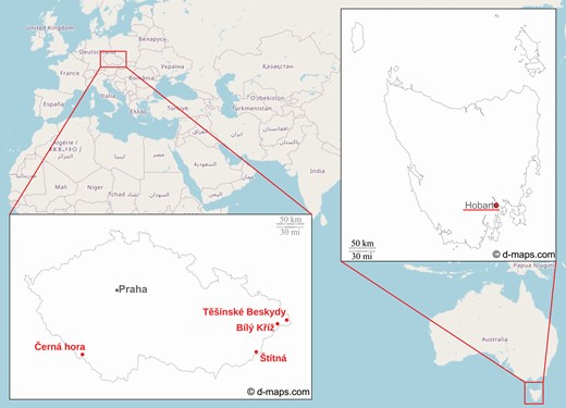
Locations of study sites (labelled in red) providing inputs for this study.
2.2 TLS and 3D tree reconstruction
TLS scans for each tree species were obtained during three independent field campaigns. Technical characteristics of each TLS acquisition are summarized in Table 2. The reconstruction algorithm consists of the following four steps (illustrated in Fig. 2): (i) segmentation of a TLS tree point cloud separating wooden parts from foliage, (ii) reconstruction of trunk and branches (Sloup 2013) based on the point cloud of wooden parts, (iii) distribution of foliage within the tree crown using the points of foliage cloud as attractors and (iv) generation of a 3D representation by merging the reconstructed wooden and foliage objects (Janoutová et al. 2019).
Overview of technical specifications of TLS used for tree scanning and their settings.
| TLS parameter | Černá hora | Hobart | Těšínské Beskydy |
|---|---|---|---|
| Scanner | OPTECH Ilris-36D | Trimble TX8 | Riegl VZ-400 |
| Manufacturer | Teledyne Optech, Vaughan, ON, Canada | Trimble, Sunnyvale, CA, USA | RIEGL Laser Measurement Systems, Horn, Austria |
| Wavelength [µm] | 1.5 | 1.5 | 1.5 |
| Maximum field-of-view | 40° × 40° | 360° × 317° | 360° (azimuth) 100° (30°–130°; zenith) |
| Data acquisition | 2009 | 2017/2018 | 2019 |
| Scanning design | • Each tree was scanned from two opposing positions, recording the first and the last echo return with the point sampling distance of 2 cm. | • Multi-scans from several (4–10) positions. • Point spacing of 11.3 mm at distance of 30 m. | • Multi-scans from the centre and four quadratic directions of the plot. • One upright and one tilted scan at every position to cover the whole hemisphere around the scanner. • Several beech trees were separated from complex TLS scenes. |
| Processing | • Point clouds of first and last returns of each individual tree were aligned and co-registered using the PolyWorks IMAlign module (InnovMetric Software Inc., Quebec City, QC, Canada). | • Point clouds of first and last returns of each individual tree were aligned and co-registered using a scan-to-scan matching in Trimble Realworks 10.1. (Trimble, Sunnyvale, CA, USA). | • Point clouds of multiple returns of each individual tree were aligned and co-registered and processed in RiScan Pro (RIEGL Laser Measurement Systems, Horn, Austria). |
![Methodological steps of the 3D reconstruction approach, illustrated by the case of a spruce (from left to right): (i) TLS tree point cloud segmentation (A), (ii) reconstruction of wooden parts [trunk and branches, (B)], (iii) distribution of foliage within the tree crown [TLS points acting as attractors, (C)], and (iv) generation of a 3D representation (D).](https://oup.silverchair-cdn.com/oup/backfile/Content_public/Journal/insilicoplants/3/2/10.1093_insilicoplants_diab026/3/m_diab026_fig2.jpeg?Expires=1716268970&Signature=mcRveEgy55GKTKOD7V-JgpXdSj0PfifgGZiofmLe8DBnRJAqocXfAd8MVaRDLTmov7r55OT27G7rjxpXUXvrtcn0OksRzwubJPgacpvilwEnBx6i5CdfJ9tN8p9dksmBEOkKuD5MOJT0oA87ILbJ3fpA8bCV56za-Y3ztYLTHHHaIq-22tT-13QFod5xGaQivjjEaJUr~TfcB0luhjHS4J6VwrkWTx9IOUdqQ2-zZjHDYE4bbOYBcHGJxW6mlP1A9CFDuhWIf2QqtUCoiTZEqM4jRkgwnbTxw6UY3zMFhEvmyCflV1mU-DWZoKjIq52TeJAxLmCxUhG0m2bM-l1bqw__&Key-Pair-Id=APKAIE5G5CRDK6RD3PGA)
Methodological steps of the 3D reconstruction approach, illustrated by the case of a spruce (from left to right): (i) TLS tree point cloud segmentation (A), (ii) reconstruction of wooden parts [trunk and branches, (B)], (iii) distribution of foliage within the tree crown [TLS points acting as attractors, (C)], and (iv) generation of a 3D representation (D).
The first step of our tree reconstruction method (i.e. segmentation of TLS point clouds) was different for each tree species due to technical differences in laser scanners and their settings.
The PolyWorks IMSurvey module was used to filter out individual Norway spruce tree point clouds and to separate wooden and foliage points based on intensity of the reflected laser signals. Considering that green foliage reflects about 10 % and wooden parts as much as 50 % of the laser signal at 1.5 µm, we determined the intensity thresholds between foliage and wooden parts per scan from first and last returns of two opposite scanning positions separately (Janoutová et al. 2019).
The white peppermint TLS points of each tree were semi-automatically separated into two groups: (i) points of trunks and branches and (ii) points representing green foliage. The separation was done, as in the previous case of Norway spruce, by thresholding scans of every scanning position separately in CloudCompare software version 2.9 (CloudCompare 2017). After the separation of wooden parts and foliage points, the scans of all measuring positions were merged and manually cleaned for obvious outliers (Malenovský et al. 2021).
We were, unfortunately, unable to apply the thresholding approach for separating woody and foliage parts in the case of European beech, because the TLS intensity values did not have the required bimodal distribution. The separation was, therefore, done manually. Since it is a time consuming process when usual 2D view methods (e.g. editing in CloudCompare) are used, we improved the efficiency of the manual editing by employing the LidarViewer software (Kreylos et al. 2008) built on top of the Virtual Reality User Interface (Vrui) toolkit (Kreylos 2008). The main advantage of using the 3D virtual reality approach is its capability of direct 3D interactions with points in the entire point cloud (i.e. whole scanned plot) at adjustable spatial scales. This allows for effective and accurate distinction, selection and export of individual points representing trees’ wooden and foliage parts. Using the 3D virtual reality technique significantly shortened the time required for the manual separation to approximately 1 day per tree, compared to at least 7 days when using a conventional 2D viewing method.
The second step (i.e. reconstruction of trunk and branches) uses an automated algorithm based on the method of Verroust and Lazarus (1999) and can be summarized in three consecutive parts: (i) component identification, (ii) component analysis and (iii) connecting components. Detailed description of all parts in the wood reconstruction algorithm is in the study of Sloup (2013). Although this algorithm was originally designed for Norway spruce, here it was tested on other tree species. In the end, its application to broadleaf tree species required only minor modification of input parameters. Some reconstructed parts were slightly deformed, e.g. too-thick or too-thin trunk and branches, but these insufficiencies were corrected by optimizing the input parameter called distanceLimit (section 4.2 in Sloup 2013), which prevented the algorithm from interconnecting points of different branches. The algorithm failed only in a special case, when the tree trunk was split into two equally thick parts at the very bottom. The wooden point cloud had to be split in two logical parts by an operator and the reconstruction was then run for each part separately.
The third step of our algorithm (i.e. distribution of 3D foliage elements − leaf or needle shoots) is conducted in the following three parts: (i) calculation of foliage elements’ positions and their angular orientation, (ii) division of foliage into age classes (only if required, i.e. for evergreen tree species) and (iii) positioning of foliage elements and their angular orientations (Fig. 3). Detailed description of all parts is available in the study of Janoutová et al. (2019). Again, the algorithm for distribution of 3D foliage elements was primarily designed for Norway spruce and here it was customized to suit the two broadleaf species. The modification consisted of two adjustments. First, leaf angular orientation was based on predefined LAD functions, because direct measurements of individual leaves’ orientation was not available. Instead, we defined the angular orientation according to indirect optical measurements as erectophile for eucalyptus family species (Danson 1998; Pisek and Adamson 2020) and planophile for beech trees (Chianucci et al. 2018; Liu et al. 2019a). This modification was implemented by loading the LAD probability function from an external file, which allows the algorithm to switch to another LAD function whenever needed. Second, the separation of foliage objects into two age classes was not applied. Even though white peppermint is an evergreen species and its trees retain more than one generation of leaves, this feature was disabled due to a lack of data. It can be enabled once information about the spatial distribution of current and older leaves becomes available.
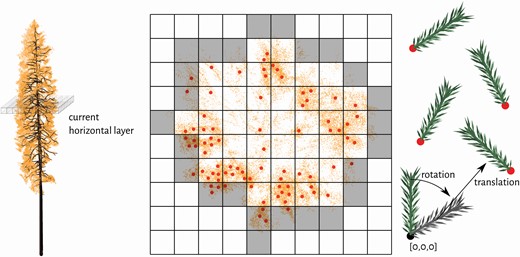
Illustration of the algorithm for distribution of Norway spruce shoot representations within a tree crown in three steps: (i) calculation of shoots’ positions (red dots) and rotations, (ii) division of shoots into two age classes (current-year and older) and (iii) translation of each shoot from its original coordinates (the black dot) into predefined positions (red dots) and angular orientations. The grey voxels correspond to the convex hull of a tree crown in the visualized horizontal layer and serve for identification of the current-year shoots’ positions.
The needle shoot representation used in this study was created for the RAdiation transfer Model Intercomparison exercise (RAMI IV) (Table 3; Widlowski et al. 2015), then adapted and simplified for use in RT modelling in collaboration with DART scientists. Three-dimensional representation of a white peppermint leaf was created based on an average shape and size of actual leaves depicted in the guide to the eucalypts of Tasmania by Wiltshire and Potts (2007). Creation of a 3D object representing a European beech leaf was carried out based on field measurements acquired at the Štítná study site in 2011. Several beech leaves were scanned using a flatbed scanner at 600 dpi resolution and their mean areas were calculated from the scans. In both cases, the digital representation was created in Inkscape version 0.92 (Inkscape Project 2017), simplified and then converted into a 3D object in Blender version 2.79 (Blender Online Community 2017) (Table 3).
Foliage objects used to generate 3D tree representations. The leaf area and number of facets in each foliage object were exported from the Blender software (Blender Online Community 2017).
| Tree type | Norway spruce | White peppermint | European beech |
|---|---|---|---|
| Detailed leaf/shoot | 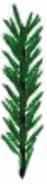 1 1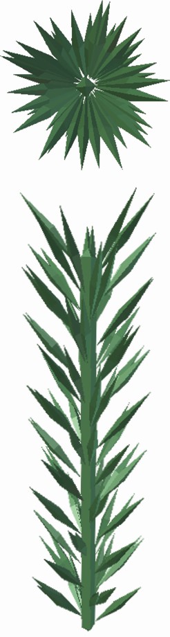 |  |  |
| Simplified leaf/shoot |  |  |  |
| Leaf area [cm2] | 38.022 | 2.73 | 12.21 |
| Number of facets (detailed/simplified) | 8243/16 | 33/2 | 202/6 |
| Tree type | Norway spruce | White peppermint | European beech |
|---|---|---|---|
| Detailed leaf/shoot | 1 | | |
| Simplified leaf/shoot | | | |
| Leaf area [cm2] | 38.022 | 2.73 | 12.21 |
| Number of facets (detailed/simplified) | 8243/16 | 33/2 | 202/6 |
1According to Widlowski et al. (2015).
2Outer area of needles only (i.e. half of the Blender generated value) and without the central twig.
3Sum of all twig and needle facets.
Foliage objects used to generate 3D tree representations. The leaf area and number of facets in each foliage object were exported from the Blender software (Blender Online Community 2017).
| Tree type | Norway spruce | White peppermint | European beech |
|---|---|---|---|
| Detailed leaf/shoot | 1 | | |
| Simplified leaf/shoot | | | |
| Leaf area [cm2] | 38.022 | 2.73 | 12.21 |
| Number of facets (detailed/simplified) | 8243/16 | 33/2 | 202/6 |
| Tree type | Norway spruce | White peppermint | European beech |
|---|---|---|---|
| Detailed leaf/shoot | 1 | | |
| Simplified leaf/shoot | | | |
| Leaf area [cm2] | 38.022 | 2.73 | 12.21 |
| Number of facets (detailed/simplified) | 8243/16 | 33/2 | 202/6 |
1According to Widlowski et al. (2015).
2Outer area of needles only (i.e. half of the Blender generated value) and without the central twig.
3Sum of all twig and needle facets.
Within the last step, the reconstructed wooden and foliage objects were merged together to form the final 3D tree representation.
2.3 Comparison of different tree parameterizations
There are several levels of a tree abstraction applicable in RT simulations, starting from a highly detailed geometrically explicit tree up to a simple generic tree with a crown represented as a turbid media. We simulated forest reflectance of three different tree representations in the DART model (Gastellu-Etchegorry et al. 1996, 2015, 2017) to demonstrate the impact of tree 3D structure details on the canopy reflectance. In the simplest parameterization tree crown shapes are approximated as regular 3D geometric shapes built out of voxels filled with a turbid medium. The turbid medium voxels are filled with an infinite number of infinitely small leaves characterized by predefined leaf optical and structural properties. Structural properties are defined primarily by leaf area index (LAI) and LAD, both specified either per tree or per canopy of the entire simulated scene. Other controlling parameters are distribution of empty voxels (i.e. canopy air gaps) and leaf volume density inside a voxel, both mimicking variable foliage clumping, that can be specified either per crown or according to crown vertical level. In the most detailed and precise tree parameterization the 3D tree representations are built as described in the previous sections, i.e. composed out of geometrical primitives (facets) representing foliage and wooden parts. The DART model also allows users to combine both approaches. Technical details on different tree parameterizations offered in DART are summarized in the DART User’s Manual (Gastellu-Etchegorry 2021) or in Janoutová et al. (2019).
To demonstrate the impact of differently detailed 3D tree abstractions on the DART-simulated top-of-canopy reflectance, we created for each tree species a set of three forest scenes ranging from the most complex to the most simplest 3D representation. Details of tree structural parameterizations were maintained and generalized as follows: (i) 3D detailed tree representations were retained as geometrical facets (i.e. a ‘3D detailed’ scenario); (ii) 3D detailed tree representations had foliage transformed into turbid medium (i.e. a ‘turbid’ scenario); and (iii) predefined simple 3D tree crown shapes, in our cases ellipsoidal, were filled with a turbid medium and contained simple straight trunks without branches (i.e. a ‘simple’ scenario).
In some cases, the 3D tree representations had to be spatially scaled, because the TLS data were acquired for trees of different height than the site for which RT simulations were performed. This was done by scaling dimensions of the input TLS point clouds, in the case of Norway spruce trees by scaling factor 0.6 and in the case of European beech by scaling factor 0.7 (white peppermint trees were kept unscaled). The scaling was employed to keep the scene dimensions fixed to 10 × 10 m across the species and to achieve comparable canopy cover (CC, 80 %) while using at least four individual trees in the scene (Table 4).
DART scene parameters used to simulate forest reflectance of three species: Norway spruce, white peppermint and European beech.
| Species | Norway spruce | White peppermint | European beech |
|---|---|---|---|
| Scene size [m × m] | 10 × 10 | 10 × 10 | 10 × 10 |
| Cell size [m] | 0.2 | 0.2 | 0.2 |
| CC [%] | 80 | 80 | 80 |
| Scene LAI [m2·m−2] | 8 | 8 | 8 |
| Number of trees in scene | 10 | 5 | 4 |
| Species | Norway spruce | White peppermint | European beech |
|---|---|---|---|
| Scene size [m × m] | 10 × 10 | 10 × 10 | 10 × 10 |
| Cell size [m] | 0.2 | 0.2 | 0.2 |
| CC [%] | 80 | 80 | 80 |
| Scene LAI [m2·m−2] | 8 | 8 | 8 |
| Number of trees in scene | 10 | 5 | 4 |
All other input parameters (e.g. optical properties, CC and scene LAI) were unified to ensure that the results are influenced only by the tree structural parametrization. The DART scene input parameters are summarized in Table 4. The foliage optical properties were simulated in the PROSPECT-D leaf RTM (Féret et al. 2017) according to input parameters are listed in Table 5. The simulated directional-hemispherical leaf reflectance and transmittance are shown in Fig. 4 (left). The optical properties for woody twigs, stem bark and ground (Fig. 4, right) were measured during a field campaign in 2016 at the study site Bílý Kříž (Table 1; Homolová et al. 2017).
Input parameters used in PROSPECT-D leaf RTM to simulate leaf optical properties (i.e. reflectance and transmittance).
| Parameter | Leaves/needles |
|---|---|
| Chlorophyll content [µg·cm−2] | 43.15 |
| Carotenoid content [µg·cm−2] | 9.18 |
| Dry matter content [g·cm−2] | 0.017 |
| Water content [g·cm−2] | 0.021 |
| Structural parameter [−] | 1.9 |
| Fraction of brown pigments [−] | 0 |
| Anthocyanin content [µg·cm−2] | 0 |
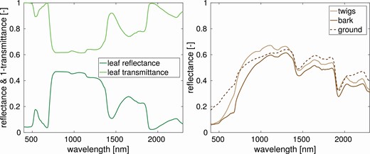
Leaf reflectance and transmittance spectra generated for DART simulations by PROSPECT-D (left), and measured directional-hemispherical reflectance of shoot twigs, stem bark and ground cover (right). These optical properties were used in all scenarios.
3. RESULTS AND DISCUSSION
3.1 3D tree representations
The results reported in Table 6 confirm the successful extension and application of the algorithm developed in Janoutová et al. (2019) to the other two tested broadleaf tree species. Four individuals per species were successfully reconstructed despite that white peppermint (Fig. 6) and European beech (Fig. 7) occupy contrasting habitats and have very different tree crown architectures compared to Norway spruce. Additionally, the TLS input data of each species were acquired using an instrument of different technical design, specifications and setup, and that data also were processed differently. This suggests that our reconstruction algorithm is sufficiently robust to use TLS data that differ in terms of acquisition parameters and processing levels. It also can handle significant variation in trunk and branch shapes, as well as in the foliage spatial and angular distribution that appears among, but also within, the biological species, as documented in Figs 5–7 and Table 6.
Characteristics of 3D tree representations produced for the three investigated tree species. The characteristics relate to trees with detailed forms of shoots or leaves, as listed in Table 3. Differences in tree LAI are due to different requirements of target applications using the 3D tree representations.
| Parameter | ||||||
|---|---|---|---|---|---|---|
| Tree height [m] | Crown length [m] | Crown diameter in x-axis [m] | Crown diameter in y-axis [m] | Number of wood facets | Number of leaf facets | |
| Norway spruce (LAI 12) | ||||||
| S. tree 1 | 15.0 | 14.5 | 2.88 | 2.48 | 112 448 | 11 750 240 |
| S. tree 2 | 15.3 | 10.5 | 3.03 | 3.01 | 106 112 | 15 757 352 |
| S. tree 3 | 16.4 | 14.2 | 4.13 | 3.93 | 186 432 | 28 014 352 |
| S. tree 4 | 14.8 | 14.6 | 4.56 | 4.27 | 197 760 | 28 594 448 |
| White peppermint (LAI 5) | ||||||
| P. tree 1 | 9.44 | 4.86 | 4.09 | 3.60 | 87 122 | 4 203 672 |
| P. tree 2 | 10.47 | 7.20 | 6.76 | 6.57 | 147 374 | 10 611 645 |
| P. tree 3 | 15.97 | 5.72 | 8.15 | 7.80 | 124 098 | 17 943 090 |
| P. tree 4 | 13.19 | 10.56 | 6.97 | 8.60 | 281 622 | 6 957 225 |
| European beech (LAI 12) | ||||||
| B. tree 1 | 21.2 | 18.32 | 7.36 | 8.30 | 50 820 | 21 756 006 |
| B. tree 2 | 27.2 | 16.60 | 11.12 | 8.21 | 100 322 | 20 288 678 |
| B. tree 3 | 22.3 | 13.66 | 5.86 | 7.88 | 132 330 | 20 057 186 |
| B. tree 4 | 16.8 | 15.72 | 5.70 | 6.22 | 37 686 | 23 561 886 |
S, Spruce; P, Peppermint; B, Beech.
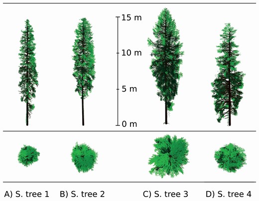
Four Norway spruce tree 3D representations (A-D) reconstructed from TLS data point clouds acquired with an OPTECH Ilris-36D instrument. Colour rendering indicates wooden parts in dark brown, current-year needle shoots in light green and older needle shoots in dark green (Janoutová et al. 2019).
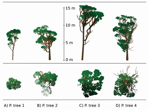
Four white peppermint tree 3D representations (A-D) reconstructed from TLS data point clouds acquired with a Trimble TX8 instrument. Colour rendering indicates wooden parts in brown and leaves in green.
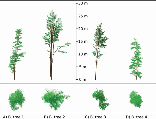
Four European beech tree 3D representations (A-D) reconstructed from TLS data point clouds acquired with a Riegl VZ-400 instrument. Colour rendering indicates wooden parts in brown and leaves in green.
The main advantage of the algorithm is its ability to reconstruct an extensive variety of trees across and within given species from a relatively small amount of input data. The largest structural variability originates from structural differences between tree species, spanning in this study from regularly organized spruce crowns, with branches growing in whorls carrying symmetrical needle shoots; to irregularly distributed large and dense clumps of broad leaves, characteristic for white peppermint; and to smaller, sparse leaf clumps of European beech organized more regularly in the vertical dimension. Nonetheless, additional within-species variability originates from ecological interactions and environmental disturbances, such as competition among neighbouring trees for resources (e.g. for photosynthetically active radiation, water and nutrients) causing variation in tree height (dominant vs suppressed trees) or strong wind gusts causing irregularities in tree crowns (e.g. missing and broken branches). The algorithm seems capable of capturing all these naturally occurring biotic and abiotic impacts.
The only required algorithm inputs are the following: TLS point clouds, information about foliage distribution (e.g. LAD function) and a representative 3D object of crown foliage elements. Generally speaking, the accuracy achieved is greater for denser and more precise TLS scans. Although recent advances in TLS technology allow for quick acquisitions of high-density point clouds, its deployment in a naturally dense forest comes up against its technical limits. Distances between scan positions, from scanned trees, and between the scanner and different parts of crowns cannot be unified, thus causing unequal point cloud density and varying intensity of laser reflections. This results in a lower point cloud quality, which in turn makes automated separation of wooden parts and foliage via intensity threshold in some cases inapplicable. TLS data with calibrated intensity of laser returns can significantly accelerate this separation (Kaasalainen et al. 2009, 2011; Calders et al. 2017) by allowing the threshold application on the whole tree point cloud simultaneously. Additionally, scanning inside a forest stand causes gaps in data and occlusion, as some parts of a scanned tree might be obscured by other tree parts and forest objects (Bremer et al. 2013; Sloup 2013). Although the reconstruction of wooden parts accounts for the existence of such obstruction, it had to be optimized per species. When too many large gaps occurred in TLS point clouds, especially of broadleaf species, the algorithm occasionally produced architectural anomalies (e.g. incorrectly connected branches, strange branching angles, or a secondary trunk connected to some branches growing from the primary trunk). We also encountered a main trunk being split into multiple large branches, despite that the wood reconstruction algorithm has been designed to work only with a single trunk. It happened in the case of beech tree no. 2 (Fig. 7B), which has two main trunks. The point cloud of trunks had therefore to be split into two parts, and their reconstruction was carried out separately. The two reconstructed wooden parts were afterwards merged manually in the Blender software (Blender Online Community 2017). Regardless of these rather specific pitfalls, only in a few cases did the algorithm run into a problem. In the majority of cases, a minor readjustment of the input parameter distanceLimit (section 4.2 in Sloup 2013) was sufficient to enable the algorithm to find the right solution for any of the three tested species.
Another mandatory input is the information about foliage spatial and angular distributions. The spatial distribution of leaves is computed directly from the actual density of a foliage point cloud, but the absolute amount of leaf objects is controlled by an operator defining a desirable tree LAI. The easiest way to set the foliage angular distribution is through a predefined LAD function (e.g. spherical, planophile, erectophile; Wit 1965). Direct field measurements of leaf inclination angle in conifers are rarely available (e.g. Barták 1992; Barták et al. 1993), unlike for broadleaf tree species where methods to measure leaf inclination angle from digital photography have been developed (Ryu et al. 2010; Chianucci et al. 2018; Pisek and Adamson 2020). It would be very efficient if a tree-specific leaf angular distribution could be derived directly from the TLS point cloud. While focusing on broadleaf tree species, the first methodological attempts of this kind have been published by Zheng and Moskal (2012), Liu et al. (2019a), Vicari et al. (2019) and Stovall et al. (2021). The latter approach of Stovall et al. (2021) also performs the segmentation of leaves and wooden tree parts, but neither of our TLS data has sufficient point density to test the method. However, it will be desirable to test that approach and possibly to implement it in our future processing once suitable TLS data are acquired.
Finally, creation of the 3D foliage element object is not a limiting factor. It is straightforward and, especially for broadleaf species, easy to prepare such an object from 2D scans of leaf blades (Table 3). Nevertheless, inclusion of additional and different foliage objects representing, for instance, different age classes or leaf types might be more challenging. Their positions and angular orientations need to be known prior to their distribution within a crown, and currently these cannot be derived from any indirect observation like TLS. We were able to implement needle shoots of two age classes for Norway spruce trees, but only because we had unique destructive field measurements provided in Barták (1992) and Barták et al. (1993). The same treatment would be desirable also for evergreen white peppermint trees, but no specific information on the amounts and positions of newly developed and older leaves was available.
3.2 Comparison of reflectance for different tree abstractions
The comparison showed that the simpler parameterization scenarios (i.e. turbid and simple) produced for all tree species a higher DART-simulated forest reflectance in the near-infrared (NIR) region (720–800 nm) than the 3D detailed scenario (Fig. 8). The relative NIR reflectance difference is between 4 % and 30 % in the case of turbid scenarios and between 52 % and 130 % in the case of simple scenarios (Fig. 8). Overestimations can be observed also around the green peak (centred at 540 nm), where the relative reflectance difference varied between 0 % and 33 % in the case of turbid scenarios and between 17 % and 135 % in the case of simple scenarios (Fig. 8). Contrary to this, the simpler scenarios tend to underestimate reflectance of the 3D detailed scenarios within the red chlorophyll absorption region (650–680 nm), where the relative difference is between −22 % and −33 % in the case of turbid scenarios and between −31 % and −69 % in the case of simple scenarios (Fig. 8). Slightly smaller underestimation is observed in the blue region (400–500 nm), revealing the relative difference between −3 % and −20 % in the case of turbid scenarios and between −26 % and −40 % in the case of simple scenarios (Fig. 8). Overall, reflectance of turbid scenarios differs from 3D detailed less than simple scenarios (Fig. 9). Visualisations of 3D forest scenes and corresponding nadir simulated images for all species and scenarios are shown in Supporting Information—Figs S1–S3.
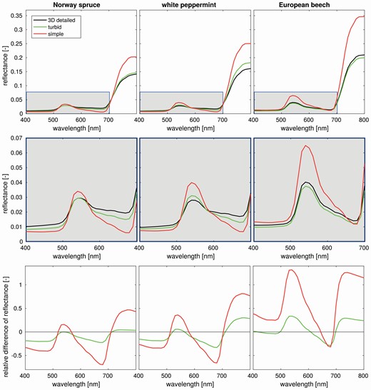
Comparison of DART-simulated nadir reflectance signatures of three scenarios for each investigated species. The scenarios vary in tree abstractions: (i) 3D detailed tree representations (3D detailed), (ii) 3D detailed tree representation transformed into a turbid medium (turbid) and (iii) predefined simple tree crown shapes filled with a turbid medium and simplified trunks (simple). At the bottom row are relative differences from the 3D detailed reference scenario.
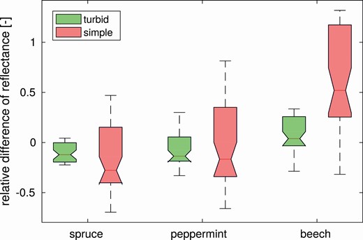
Relative difference of DART-simulated nadir scene reflectance between the reference 3D detailed scenario and two simpler scenarios (turbid and simple) for each species. Description of scenarios is available in the caption of Fig. 8.
A similar trend was observed when investigating multi-angular distributions of DART-simulated forest canopy reflectance. Polar graphs in Fig. 10 show differences between the scenarios in the NIR region (represented here by a single wavelength of 800 nm), where the structural aspects have the largest impact. The relative reflectance differences from the reference 3D detailed scenarios are higher in the case of simple scenarios, ranging between 11 % and 89 %, than for the turbid scenarios where the difference is between −18 % and 20 % (Fig. 10). In all cases of turbid scenarios, the hot spot region reflectance is underestimated between −12 % and −18 %. The Norway spruce and European beech turbid scenarios are overestimated at the extreme zenith viewing angles by 5 % up to 15 %. The white peppermint turbid scenario demonstrates a different behaviour, its reflectance is overestimated around nadir viewing angles by about 13 % and underestimated in extreme zenith viewing angles by about −12 %. In all three cases of simple scenarios, the relative difference shows reflectance overestimation, with the hot spot region being overestimated by around 11 %. Additionally, reflectance of simple scenarios differs from the reference of 3D detailed forest abstractions more heterogeneously across simulated viewing angles than turbid scenarios.
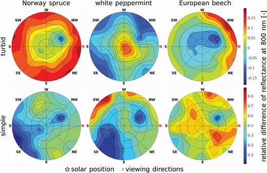
Relative differences in multi-angular distribution of simulated forest canopy reflectance at 800 nm between the complex scenario with 3D detailed tree abstractions (3D detailed) and the two simpler scenarios. Description of the simpler scenarios is available in the caption of Fig. 8.
The differences in simulated reflectance of three forest abstractions show that the reconstruction of a 3D detailed tree representation plays an important role in achieving accurate airborne and satellite spectral data simulations. The tree abstraction using predefined simple tree crown shapes filled with a turbid medium and simplified trunks is unable to reliably substitute the 3D detailed tree representation. The reflectance differences were also noticeable when the 3D detailed tree representations were converted in a canopy turbid medium. However, the conversion into turbid medium saves time and decreases computational demands (summarized in Table 7), e.g. in case of spruce scene the 3D detailed scenario took 12 h and 33 min with 155 GB RAM at 30 CPU to be simulated, while the turbid scenario needed only 1 h and 59 min with 21 GB RAM at 20 CPU. In some applications, this might be a sufficient justification for trading the reflectance accuracy by the computational feasibility.
DART model computational demands for simulating forest scenes of three species: Norway spruce, white peppermint and European beech.
| Parameter | 3D detailed | Turbid | Simple |
|---|---|---|---|
| Product | Simulated forest bidirectional reflectance factors between 400 and 800 nm with a step of 10 nm | ||
| Computation demands [per simulation] | 30 CPU | 20 CPU | 10 CPU |
| 155–7 GB RAM | 22–11 GB RAM | 62–24 GB RAM | |
| 753–35 min | 120–48 min | 394–184 min | |
| DART version | 5.7.9. v1192 |
3.3 RS applications
Some optical RS applications are deeply rooted in computer-based RTMs that simulate light interactions (absorption and scattering) with 3D objects placed inside a virtual scene (e.g. Liu et al. 2019b; Lukeš et al. 2020; Malenovský et al. 2021). Such modelling requires structural representations of the studied objects that are sufficiently detailed to enable RTM to resolve light interactions at spatial scales appropriate to specific research questions (Janoutová et al. 2019; Malenovský et al. 2020, 2021). Numerous RS RTM-based applications, such as simulation of terrestrial and airborne laser scans for validation and calibration of above-ground forest biomass estimations (Disney et al. 2018) or scaling of leaf optical signals to the top of forest canopies (Malenovský et al. 2019; Lukeš et al. 2020), require reconstructed 3D abstractions of trees.
In Appendices A and B, we provide two case studies as examples demonstrating use of the 3D tree representations created in this work for (i) interpretation of airborne and space-borne spectral RS data and (ii) investigating influence of forest structures, particularly woody components, on remotely sensed SIF signal. Both applications are computationally highly demanding procedures. To reduce their computational time, the 3D tree representations had to be created from a minimal number of required geometrical facets. Inasmuch as the original algorithm outputs were constructed from far too many facets (Table 6), we separated the part distributing the foliage objects within a tree crown as a stand-alone algorithm. This offered a quick and easy way to replace the foliage objects with others having an optimal lower number of facets (see Table 3) whenever needed.
The first example shows retrievals of biophysical parameters of Norway spruce forest stands at the Bílý Kříž study site (Table 1 and Fig. 1) from hyperspectral RS images (Fig. 12) by means of an RTM inversion (Fig. 11). The 3D spruce representations of this study (Fig. 5) were used to create a set of about 20 000 forest scenes, reassembling the existing forest architecture and biochemistry variations (Table 8), and to simulate in DART their reflectance spectral signatures as measured from airborne sensors. A support vector regression algorithm was then trained with the DART simulations and subsequently applied on real hyperspectral airborne images of the study site to quantify contents of leaf chlorophylls, carotenoids and water, as well as LAI (Fig. 13). Appendix A provides a detailed methodological description and results of this case study.
DART parameters and computation demands of Norway spruce forest scene simulations.
| Parameter | Value |
|---|---|
| Scene size [m × m] | 10 × 10 |
| Cell site [m] | 0.5 |
| Tree model | TLS-reconstructed 3D geometrical representation transformed into turbid voxel |
| CC [%] | 50–65–80–95 |
| Number of trees in scene | 6–9–10–13, depending on CC |
| Scene LAI [m2·m−2] | 3–10 with step 1 |
| Product | Simulated forest bidirectional reflectance factor images |
| Computation demands | • 22 273 simulations • 20 simulations in one sequence • 8 CPU per sequence (2 simulations running in parallel) • 25 GB RAM per sequence • 2 days per sequence |
| DART version | 5.6.2 |
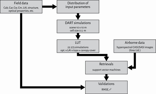
Flowchart outlining retrieval of vegetation parameters from RS images. Cab, leaf chlorophyll content; Car, leaf carotenoid content; Cw, leaf water content; Cm, leaf dry matter content; opt, optical properties; topo, topography; r2, coefficient of determination.
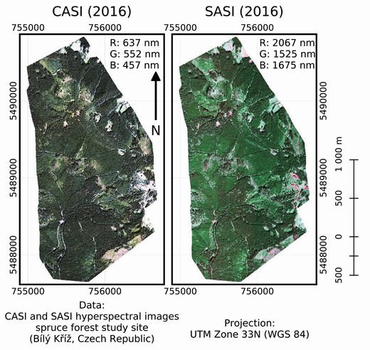
Hyperspectral airborne images of Bílý Kříž study site acquired on 31 September 2016. Image from CASI (wavelength range: 380–1050 nm) and SASI (wavelength range: 950–2450 nm).
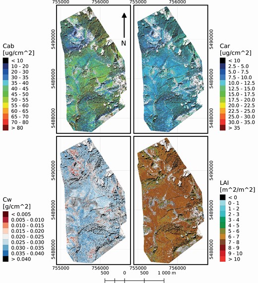
Maps of leaf chlorophyll content (Cab), leaf carotenoid content (Car) retrieved from the CASI airborne image data, and leaf water content (Cw), and LAI retrieved with a support vector regression trained with DART-modelled reflectance from the SASI airborne imagery (see Fig. 12).
The second example presents a virtual sensitivity study investigating impact of wooden canopy parts (trunks and branches) on SIF of white peppermint forest stands simulated in DART (Gastellu-Etchegorry et al. 2017). Because it is physically impossible to remove wood and measure the effect of its absence or presence in a real forest, the RT computer simulations were the only way to achieve this objective (Malenovský et al. 2020, 2021). Three-dimensional tree representations of four white peppermint trees (Fig. 6) were used to create four DART virtual scenes: (i) a dense stand (ground CC about 80 %) containing wood (trunk and branches), (ii) the same stand without wood (only leaves), (iii) a sparse stand (CC about 40 %) containing wood and (iv) the same sparse stand without wood. Subsequently, RTMs were employed to simulate SIF signals, as observed by an airborne RS sensor above a forest canopy, and also a portion of SIF photons escaping from the canopy in all directions and in the nadir viewing direction. Comparison of the outcomes for simulations with and without wood enabled us to reveal wood’s potential impact. Appendix B provides a detailed description of the methodology and its results.
The future perspective of this work entails a combination of TLS data with, or even its replacement by, airborne laser scanning (ALS) measurements. A larger spatial extent of ALS acquisitions would allow for efficient reconstruction of entire forest stands. As suggested by Jurík (2019), the ALS data could be used to segment a forest into individual trees and then to select the best performing tree 3D reconstruction for each detected tree from a library based on species and tree proportions (e.g. tree height, crown width and shape). Use of ALS data requires new methods capable of creating individual tree 3D representations from point clouds of much lower density, but it represents a significant step forward towards fully automated reconstruction of large virtual forest stands.
4. CONCLUSION
The algorithm, originally developed for detailed 3D reconstruction from TLS scans of coniferous Norway spruce trees, was successfully extended and applied to two broadleaf tree species, white peppermint and European beech. The extension required a few simple modifications of the previous algorithm, but no significant changes had to be introduced. Although the reconstruction proved to be robust and applicable to the three species of this study, it requires further testing, especially for tree species of irregular shapes growing in extreme environmental conditions (e.g. high-altitude treelines or high-latitude boreal forests).
Our detailed 3D representations of trees with complex architectures improved existing and enabled new RS applications and sensitivity studies that were unfeasible using previous, much simpler tree abstractions. This capability is highly relevant for synergistic use of imaging unmanned aircraft systems operating at very high spatial resolutions of only a few centimetres. With the rapid development of ALS RS techniques and improving performance of computational resources, it might soon be possible to reconstruct and simulate even whole forest stands of a given study area. A fundamental prerequisite for achieving this goal is a fully automated algorithm for reconstructing trees.
SUPPORTING INFORMATION
The following additional information is available in the online version of this article—
Figure S1. Visualization of Norway spruce forest 3D scenes and DART-simulated top-of-canopy reflectance images for three scenarios.
Figure S2. Visualization of white peppermint forest 3D scenes and DART-simulated top-of-canopy reflectance images for three scenarios.
Figure S3. Visualization of European beech forest 3D scenes and DART-simulated top-of-canopy reflectance images for three scenarios.
ACKNOWLEDGEMENTS
The authors would like to thank Petr Sloup and Tomáš Rebok from the Masaryk University in Brno for providing code for 3D tree wooden parts reconstruction; Luke Wallace and Samuel Hillman from the RMIT University in Melbourne for acquisition of the white peppermint TLS point clouds; and IFER–Institute of Forest Ecosystem Research, Ltd. and IFER–Monitoring and Mapping Solutions, Ltd. for providing the field data for the Těšínské Beskydy study site. Jean-Philippe Gastellu-Etchegorry, Nicolas Lauret and members of the DART team at the CESBIO Laboratory in Toulouse are acknowledged for supporting our DART modelling. We also thank three anonymous reviewers for their constructive comments that helped us to improve this manuscript.
SOURCE OF FUNDING
This work was supported by the Ministry of Education, Youth and Sports of Czech Republic within the CzeCOS program (grant no. LM2018123) and within the Inter-Excellence program (grant no. LTC20055) and by the Action CA17134 SENSECO (‘Optical synergies for spatiotemporal sensing of scalable ecophysiological traits’) funded by COST (European Cooperation in Science and Technology, www.cost.eu). The contribution of Z.M. was funded by the Australian Research Council Future Fellowship ‘Bridging Scales in Remote Sensing of Vegetation Stress’ (FT160100477).
CONFLICTS OF INTEREST
None declared.
CONTRIBUTIONS BY THE AUTHORS
R.J., L.H. and Z.M. contributed to the conception and design of the work; R.J., J.N., B.N. and M.P. collected and processed the data; R.J., L.H. and Z.M. contributed to data analysis and interpretation; R.J. performed modelling and conducted the simulations; R.J., L.H. and Z.M. contributed to drafting the manuscript; L.H. and Z.M. supervised the implementation and contributed to critical revision of the manuscript.
Appendix A. Case Study for Norway Spruce: Retrieval of Forest Biophysical Parameters From RS Spectral Observations
Inversion of vegetation RTM simulations is widely used for retrieval of specific biochemical and structural parameters, termed plant functional traits (Homolová et al. 2016; Verrelst et al. 2019). In this case study, the 3D representations of Norway spruce (Picea abies) trees were used to construct a virtual forest stand in the DART RTM (Gastellu-Etchegorry et al. 2017) with the aim of generating a large spectral database of forest reflectance signatures [look-up tables (LUT)]. Table 8 reports the basic parameters and computational requirements to simulate LUT with reflectance forest signatures in DART. A machine-learning algorithm (i.e. a support vector regression) was then trained with the LUT input/output data and subsequently applied per-pixel on airborne hyperspectral images to estimate forest biophysical and structural parameters, specifically: leaf chlorophyll a+b (Cab), total leaf carotenoid (Car) and water (Cw) contents, as well as LAI.
The methodological workflow of this case study is briefly depicted in the flowchart in Fig. 11. A comprehensive field and airborne data acquisition campaign was conducted in September 2016. Airborne images from CASI and SASI hyperspectral sensors (Fig. 12) were acquired simultaneously with the supporting field data used for: (i) parametrization of DART 3D scenes, (ii) generating the LUT and (iii) validation of retrieved biochemical and structural parameters (Homolová et al. 2017). The minimum-to-maximum ranges, measured for biochemical and structural forest parameters during the field campaign, were between 31.7 and 41.1 µg·cm−2 for Cab, 6.4 and 8.3 µg·cm−2 for Car, 0.01 and 0.02 g·cm−2 for Cw, and 5.3 and 9.3 m2·m−2 for LAI. Figure 13 shows the results of the airborne hyperspectral retrievals. The accuracy of retrieved traits was assessed with root mean square error (RMSE) and r2, gaining the following values: 8.16 and 0.37 for Cab, 1.63 and 0.20 for Car, 0.008 and 0.06 for Cw, and 1.36 and 0.61 for LAI, respectively.
Appendix B. Case Study for White Peppermint: Impact of Canopy Woody Components on Emission and Escape of Solar-Induced Chlorophyll Fluorescence
Remotely sensed SIF, a subtle optical signal originating from photosynthetic processes of green plants (Mohammed et al. 2019), is being used to improve gross primary productivity estimates of terrestrial vegetation including forests (Tagliabue et al. 2019). SIF signal, however, interacts with various forest canopy structures, which results in its intensity angular anisotropy. To investigate the potential impacts of forest structures, and in this case study the presence of canopy woody elements, we coupled the leaf fluorescence model Fluspect-Cx (Vilfan et al. 2018) with the DART canopy RTM (Gastellu-Etchegorry et al. 2017) and simulated propagation and interactions of SIF photons (i.e. SIF radiative budget) through structurally complex canopies of a dense (CC = 80 %) and a sparse (CC = 40 %) Australian white peppermint (Eucalyptus pulchella) stand. Three-dimensional representations of the stands in DART were constructed based on TLS (Table 2) of peppermint trees acquired together with optical properties of forest surfaces in the vicinity of Hobart (Tasmania, Australia; Table 1). Table 9 outlines basic input parameters and computational requirements of DART modelling. Radiative budgets and images of red (λ = 686 nm) and far-red (λ = 740 nm) SIF were simulated for the forest stands without wood (only leaves) and with the presence of wood (i.e. with trunks and branches).
DART parameters and computation demands of white peppermint forest scene simulations.
| Parameter | Value |
|---|---|
| Scene size [m × m] | 9 × 9 and 14 × 14 |
| Cell site [m] | 0.2 |
| Tree model | TLS-reconstructed 3D geometrical representation |
| CC [%] | 40–80 |
| Number of trees in scene | 3 |
| Scene LAI [m2·m−2] | 2.5 |
| Product | Images and radiative budget of SIF and bidirectional reflectance factor |
| Computation demands | • 4 simulations • 10 CPU per simulation • 8 GB RAM dense scene • 14 GB RAM sparse scene • 3.5 h dense scene • 6.2 h sparse scene |
| DART version | 5.7.6 |
We investigated the impact of wood’s presence on: (i) the top-of-canopy fluorescence emitted by photosystem I (PSI) and II (PSII) (SIFnadir(λ)PSI+PSII) and (ii) two relative canopy SIF escape factors, thereby indicating how large is a proportion of fluorescence emitted by leaves that escapes from the top of the canopy in all directions of the upper hemisphere or in a given singular viewing direction. The hemispherical SIF escape (SIFhemi(λ)esc) was computed as:
where X(λ)PSI+PSII is DART-modelled SIF exitance of PSI and PSII fluorescence [W.m−2.μm−1] at wavelength (λ), which is exiting from a simulated canopy in all viewing directions of the upper hemisphere. E(λ)PSI+PSII is total SIF emission of PSI and PSII per m2 of abaxial and adaxial leaf sides. The nadir SIF escape (SIFnadir(λ)esc) was calculated as:
where SIFnadir(λ)PSI+PSII is a DART-modelled PSI and PSII SIF radiance [W.m−2.µm−1.sr−1] at wavelength (λ) exiting from a simulated canopy in the nadir viewing direction. DART-simulated nadir images of the top-of-canopy SIF emitted by PSI and PSII at λ = 740 nm are shown in Fig. 14. A comparison of SIFnadir(λ)PSI+PSII, SIFhemi(λ)esc and SIFnadir(λ)esc simulated by DART at wavelengths of 686 and 740 nm for the dense and sparse white peppermint canopies with and without wood is shown in Fig. 15.
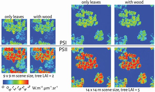
DART-simulated photosystem I (PSI) and photosystem II (PSII) SIF at λ = 740 nm. Nadir images of dense (CC = 80 %) and sparse (CC = 40 %) white peppermint (Eucalyptus pulchella) canopies (LAI = 2.5 m2·m−2) were simulated without wood (only leaves) and with trunks and branches (with wood).
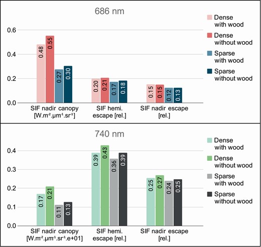
Comparison of nadir SIF (SIFnadir(λ)PSI+PSII), hemispherical (SIFhemi(λ)esc) and nadir (SIFnadir(λ)esc) escape factors simulated by DART at 686 and 740 nm for the dense and sparse white peppermint (Eucalyptus pulchella) canopies with and without wood.
The results obtained with 3D reconstructions of peppermint trees cannot be acquired through either field measurements or controlled laboratory experiments. Hence, they provide us with a unique insight in potential effects of woody components on airborne and space-borne observations of SIF. On the one hand, the results shown in Fig. 15 indicate a significant impact of wood on SIFnadir(λ)PSI+PSII for both wavelengths (particularly at 740 nm) in the case of the dense peppermint canopy. The impact in the case of the sparse canopy is also noticeable, but weaker. The same applies to SIFhemi(λ)esc at 740 nm. On the other hand, the impact of trunks and branches on SIFhemi(λ)esc at 686 nm and SIFnadir(λ)esc at 740 nm was rather small. Negligible or no impact was found in the case of SIFnadir(λ)esc at 686 nm.
