


SUMMARY
We present results of applying a local event detector based on artificial neural networks (ANNs) to two seismically active regions. The concept of ANNs enables us to recognize earthquake-like signals in seismograms because well-trained neural networks are characterized by the ability to generalize to unseen examples. This means that once the ANN is trained, in our case by few tens to hundreds of examples of local event seismograms, the algorithm can then recognize similar features in unknown records. The detailed description of the single-station detection, design and training of the ANN has been described in our previous paper. Here we show the practical application of our ANN to the same seismoactive region we used for its training, West Bohemia/Vogtland (border area Czechia-Saxony, local seismic network WEBNET), and to different seismogenic area, Reykjanes Peninsula (South-West Iceland, local seismic network REYKJANET). The training process requires carefully prepared data set which is preferably achieved by manual processing. Such data were available for the West Bohemia/Vogtland earthquake-swarm region, so we used them to train the ANN and test its performance. Due to the absence of completely manually processed activity for the Reykjanes Peninsula, we use the trained ANN for swarm-like activity in such a different tectonic setting. The application of a coincidence of the single-station detections helps to reduce significantly the number of undetected events as well as the number of false alarms. Setting up the minimum number of stations which are required to confirm an event detection enables us to choose the balance between minimum magnitude threshold and a number of false alarms. The ANN detection results for the Reykjanes Peninsula are compared to manual readings on the stations of the REYKJANET network, manual processing from Icelandic regional network SIL (the SIL catalogues by the Icelandic Meteorological Office) and two tested automatic location algorithms. The neural network shows persuasively better detection results in terms of completeness than the SIL catalogues and automatic location algorithms. Subsequently, we show that our ANN is capable of detecting events from various focal zones in West Bohemia/Vogtland although mainly the focal zone of Nový Kostel was used for training. The performance of our detector is comparable to an expert manual processing and we can state that no important event is missed this way even in case of complicated multiple events during the earthquake swarms.
1 INTRODUCTION
Continuously recording dense seismic networks produce a huge amount of data which the majority of them are redundant when processing seismic events. Seismic events, the useful part of seismic records for the most of seismological research, occur in just a small fraction of total recorded time even in episodic periods of increased seismic activity, for example, earthquake swarms. The target seismic events recorded on seismic stations may differ in few orders of amplitude and they may have fairly different shape and frequency content. Therefore, the classical STA/LTA (Short-Term Average over Long-Term Average) or other power-based detector detects also various disturbances and with the aim to detect even weak earthquakes it results in a high number of false detections. Well-performing detection algorithm minimizes false detections while preserving all important information, that is, all target seismic events. In our case we want to detect only local events with completeness magnitude as low as possible. Such reduction of data enables effective processing of events either manually or automatically. Event detection can be done in the time domain, frequency domain, by using polarization analysis or pattern matching (Withers et al.1998) or using a combination of these approaches. Artificial neural networks (ANNs) can be used in any of the listed methods. ANNs are machine learning algorithms inspired by the functionality of the human brain. The basic unit called artificial neuron simulates the behaviour of a natural neural cell as described by biologists, that is, the weighted sum of inputs generates logical output. An interconnection of neurons into network enables to solve complicated problems and the goal of the learning process is to find optimum weights for each neural input to get the desired result. ANN concept has been used in seismological applications mainly for classification or discrimination purposes (Dowla et al.1990; Romeo 1994; Tiira 1996; Esposito et al.2006; Kuyuk et al.2011; Mousavi et al.2016), phase picking (Dai & MacBeth 1997; Wang & Teng 1997; Gentili & Michelini 2006; Gravirov et al.2010; Ross et al.2018) or earthquake prediction (Panskkat & Adeli 2007; Morales-Esteban et al.2013; Reyes et al.2013). Several neural network concepts have been used for seismic event detection. Most of the works utilized shallow networks based on multilayer perceptron with one hidden layer (e.g. Wang & Teng 1995, 1997; Tiira 1999; Gentili & Michelini 2006; Madureira & Ruano 2009), but recently even very deep neural networks have been successfully applied, namely Mousavi et al. (2018) combined 2-D convolutional neural networks and bi-directional LSTM cells in a deep network with 256 000 trainable parameters. Our neural network described in Doubravová et al. (2016) takes into account the frequency character of the waveform by using narrow-band filter bank, as well as the time domain using STA/LTA in each frequency band. A sufficiently long time window used for distinguishing target seismic events from disturbing signals is very important for successful event detection. We achieved sufficient time history consideration by using a recurrent neural network. Our novel architecture named Single Layer Recurrent Neural Network (SLRNN) consists of only one layer of neurons whose outputs are fed back as inputs in the next time steps, but the recurrent inputs are delayed by various samples (the number of trainable parameters was 408). That enabled to feed information of the history of the time-series together with an actual value at the input of the network simultaneously.
It can happen that some weaker events are not detectable in the recording of a single station—due to different locations of events, local noise or disturbances, the radiation pattern of earthquake source or even technical issues (see examples in Doubravová et al.2016). Therefore our SLRNN uses multiple station detections, that is, the event detections on more stations of the network (as the human interpreters do) which increases the detection ability significantly. Most of the event detectors employed in seismological-observation practice need a special setting of parameters matching observation conditions in a particular area (e.g. local noise, frequency content of the target events and noise) to work properly. We developed our event detection method based on SLRNN as a part of the automatic processing of data from local seismic networks WEBNET and REYKJANET that are operated in two completely different tectonic areas: West-Bohemia/Vogtland earthquake-swarm region (Czechia, Central Europe) and Reykjanes Peninsula (South-West Iceland), which are characterized by swarm-like seismicity (see Section 2). The recordings of swarm activities usually contain sequences of many events tightly spaced in time or even overlapping and interfering. But such cases pose a problem for automatic algorithms and even experienced interpreters (specialists in manual processing). Our aim is to select pieces of signal with events without an attempt to separate correctly the individual events. Our SLRNN detector has been trained on data from network WEBNET. In this paper we present detection results of this detector when applied to continuous recordings from both WEBNET and REYKJANET networks.
2 TARGET AREAS AND LOCAL SEISMIC NETWORKS
2.1 West Bohemia/Vogtland
West Bohemia/Vogtland (latitude ≈49.8○N to 50.7○N, longitude ≈12○E to 13○E) is situated in the western part of the Bohemian Massif, geographically in the border area between Czechia and Saxony. It is a unique European intracontinental area that exhibits simultaneous activity of various geodynamic processes. Seismic activity is characterized by frequent occurrence of earthquake swarms, the main-shock–aftershock sequences also occur there but very rarely. Persistent swarm-like seismicity clusters in a number of small epicentral zones that are scattered in the area of about 40 km × 60 km. However, larger swarms (∼ML > 2.5) cluster predominantly in the focal zone Nový Kostel (NK), which dominates the recent seismicity of the whole region; a few tens of thousands of events were recorded there within the last 27 yr. The swarms usually consist of several thousands of weak earthquakes and their duration is from several days to two months. Notable earthquake swarms in the last 35 yr occurred in 1985/86 (with the strongest event of magnitude MLmax = 4.6), 1997 (MLmax = 2.9), 2000 (MLmax = 3.3), 2008 (MLmax = 3.8), 2011 (MLmax = 3.7), 2017 (MLmax = 3.2) and 2018 (MLmax = 3.8); an exceptional MLmax=4.4 non-swarm activity occurred in 2014. The depths of foci in the whole area range from 5 to 20 km (e.g. Horálek & Fischer 2010) but depths between 7 and 12 km are typical of earthquake swarms and main-shock–aftershock sequences (Čermáková & Horálek 2015; Jakoubková et al.2018). The region is well known by its fluid activity that is probably closely connected with the local swarm-like seismicity (e.g. Horálek & Fischer 2008; Fischer et al.2017). For summarizing information about the area in question we refer to Fischer et al. (2014). Seismicity in the West Bohemia/Vogtland region has been monitored by the WEBNET network since 1991 (Institute of Geophysics 1991; Horálek et al.2000; Fischer et al.2010). At present, WEBNET consists of 24 stations covering the area of about 40 km × 25 km. 15 stations are broad-band (equipped with Güralp CMG3-ESP sensors and Centaur digitizers by Nanometrics) with the frequency response proportional to the ground velocity from 0.03 to 100 Hz. Nine stations are short-period (LE3-D sensors and Gaia digitizers) with a flat frequency response 1.0 to 80 Hz. All the stations are operating in continuous mode with sampling frequency of 250 Hz. All 15 broad-band stations are streaming data in real time, while the short-period stations are storing data to memory cards. The amount of data is around 1.3 GB d−1 considering online stations only. Waveforms from the whole network including both online and offline stations result in approx. 2 GB d−1.
2.2 Reykjanes Peninsula
The Reykjanes Peninsula, SW Iceland (latitude ≈ 63.8○N to 64.1○N, longitude ≈ 21.5○W to 22.3○W), is the onshore continuation of the Reykjanes Ridge which is a part of the mid-Atlantic Ridge. The Reykjanes Ridge separates the two major lithospheric plates, the Eurasian Plate to the east and the North American Plate to the west. On the Reykjanes Peninsula the plate boundary extends from the southwest to the east and forms a pronounced oblique rift along the whole peninsula in length of about 65 km (Sæmundsson & Einarsson 2014). The plate motion rate on the Reykjanes Peninsula is about 20 mm yr−1 in E–W direction and about 5 mm yr−1 perpendicular to it (Geirsson et al.2010). The plate boundary is flanked by a deformation zone of about 30 km width where strain is built up by the plate movements (Einarsson 2008). The Reykjanes Peninsula is one of the most seismically active parts of Iceland, especially at the microearthquake level. Swarm-like sequences and solitary events scattered along the plate boundary, both with magnitudes mostly of ML < 3, represent a major part of seismicity on the peninsula. Large swarms took place there in 2000 (with the strongest event of magnitude MWmax = 5.9), in 2003 with MWmax = 5.3 and in 2013 with MWmax = 5.0 (Jakobsdóttir et al.2002; Jakobsdóttir 2008; Einarsson 2014). Recently, two medium swarms with magnitudes Mw = 3.8 (in 2016) and Mw = 4.1 (in 2017) occurred. Prevailing depths of the foci on the Reykjanes Peninsula are between 2 and 5 km which is much shallower compared to the focal depths in West Bohemia/Vogtland. The Reykjanes Peninsula is a highly complex geophysical structure with the interaction between volcanic and tectonic activity (Sæmundsson & Einarsson 2014), most of the Reykjanes Peninsula surface is covered by lava. The crustal fluid activity on the peninsula is clearly manifested by several geothermal fields and geothermal systems (Axelsson et al.2015). REYKJANET network (Horálek 2013) was established on the Reykjanes Peninsula in 2013 by the Institute of Geophysics and the Institute of Rock Structure and Mechanisms of the Czech Academy of Sciences with know-how, technical and material support of the University of Uppsala, Icelandic Meteorological Office (IMO) and Iceland GeoSurvey (ÍSOR). REYKJANET is aimed at monitoring interplate swarm-like seismicity in South-West Iceland. It consists of 15 broad-band stations which cover the area roughly 40 km × 20 km along the plate boundary. The stations are equipped with the Güralp CMG 40-T sensors, which are placed in special vaults, and low-power Gaia digitizers. The frequency response is proportional to the ground velocity from 0.03 to 50 or 100 Hz. All the stations operate in the continuous mode with the sampling rate of 250 Hz. The stations are supplied from batteries which are recharged from solar panels combined with wind turbines which may increase a little bit ambient noise. All the stations store the data to high capacity memory cards. Data are downloaded once in three or four months and processed afterward. The daily amount of data is some 1.3 GB, similarly to online stream of WEBNET. In addition to the REYKJANET network, seven stations of Icelandic regional network SIL (currently, a total of 68 stations spread all over Iceland), operated by IMO, have been monitored seismicity on the Reykjanes Peninsula since 1990 (Böðvarsson et al.1999). The frequency response of the SIL stations is proportional to the ground velocity from 0.2 to 40 Hz. The stations operate in the continuous mode with the sampling rate of 100 Hz. The SIL recordings are processed in IMO in near-real time by a service working 24 hrs a day.
3 DATA
The training procedure of our SLRNN detector has been described including the data used in our previous paper by Doubravová et al. (2016). Let us remind that two WEBNET data sets, (i) events of the 2008 earthquake swarm and (ii) disturbing signals of the year 2010 without swarm-like seismicity, were used to train the SLRNN; manual P- and S-wave picks were used to define an event during the training process. The training set contained both isolated and overlapping multiple events. The 2011 swarm was used for testing of the detection results. This way trained SLRNN detector has been applied to continuous data from 15 online stations of WEBNET employed in a near-real time data processing, and to continuous data from all 15 stations of REYKJANET processed in a batch after data collection. The REYKJANET network operates 2500 km away from WEBNET in entirely different seismogenic area than West Bohemia/Vogtland. Nevertheless, the extent of both networks is similar (∼ 40 km × 20 km) as well as sampling frequency (250 Hz) and a magnitude range of events, which implies that frequency content of target events is also alike. The WEBNET network has generally lower noise than REYKJANET due to installation in deep vaults and compact bedrock (compare the waveforms in Fig. 1). A rough estimate of the background noise level is 90 nm s−1 for REYKJANET and 20 nm s−1 for WEBNET, and despite the shallower depth of SW Icelandic hypocentres there is typically higher signal-to-noise ratio for WEBNET recordings. The REYKJANET network is expected to record stronger earthquakes up to magnitude ML 5.0+. The detection results for the WEBNET continuous data have been evaluated by using the WEBNET catalogues and bulletins created by precise manual data processing. In the case of the REYKJANET data, the SLRNN detector has been applied to all 15 stations. The primary source of information about local seismicity is the SIL catalogues provided by IMO (Dr Gunnar B. Guðmundsson, IMO, personal communication, 2017) which contain seismic events from the whole region of South-West Iceland. We evaluate the performance of the detector by comparing the results with (i) manual processing by a skilled expert and (ii) with automatic algorithms, mainly PePin (Fischer 2003) which is used routinely to process the WEBNET data in near-real time. PePin uses polarization analysis to find candidate onsets of P- and S-wave phases which are then associated together to define events. A set of parameters must be tuned in order to achieve good reliability of the resulting events. The algorithm naturally fails to correctly associate phases in case of complex waveforms (e.g. multiple events) which results in omitting some of the events which can be sometimes of not negligible magnitude. On the other hand, if an event is found and located by PePin, the location usually differs from the manual location by few hundreds of metres and the detection threshold for the WEBNET data is as low as ML = –1.
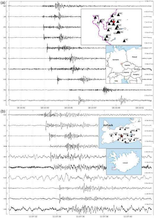
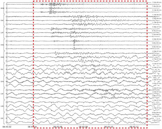
Waveform examples for (a) WEBNET (event of 2018 December 1) and (b) REYKJANET (event of 2017 July 26). Distribution of the WEBNET and REYKJANET stations is depicted in the insets (upper-right in panels a and b). Both events with local magnitude ML = 0.5 (red asterisks in the insets) were located in the centre of the seismic networks at depths characteristic of West Bohemia/Vogtland (d = 9.2 km for WEBNET) and the Reykjanes Peninsula (d = 2.5 km for REYKJANET). Only vertical components of the ground-motion velocity filtered by bandpass (BP) of 1–40 Hz at 10 stations with the best signal-to-noise ratio are depicted. All traces are scaled according to the maximum of absolute value of displayed waveform. The maximum amplitude of each trace is on the right above the traces. It is apparent that the noise is generally lower at the WEBNET stations than at the REYKJANET ones and that the seismograms from the REYKJANET stations are more complex with longer codas which makes their interpretation more demanding.
4 SINGLE STATION DETECTION—METHOD
4.1 Single Layer Recurrent Neural Network (SLRNN)
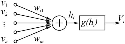
Single neuron scheme for ith neuron with inputs v1 − vn, weights wi1 − win, activation function g(.) and output Vi.1
The SLRNN consists of one neuron layer (parallel neurons) and the outputs of all neurons are fed back as inputs in the next time steps (see the scheme in Fig. 3). The outputs are applied to inputs with various delays which enables the network to get information throughout the history. After performing tests published in Doubravová et al. (2016) we conclude that eight neurons’ configuration with delays 1, 2, 4 and 8 samples is sufficient for event detection. Only three outputs of neurons are used as outputs of the whole network, the rest denoted as hidden neurons is used only for the feedback. We use output (V1) as an event detection signal, output V2 as P-wave detection and output V3 as S-wave detection. The P- and S-wave detection outputs are auxiliary and they are used only during the training process.
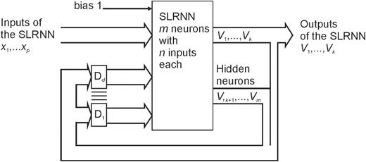
Single Layer Recurrent Neural Network with p inputs x1…xp, k outputs V1…V|$_{ k}$| and |$m-k$| hidden neurons with outputs |$V_{ k+1}...V_{m}$|. All outputs (|$V_{1}...V_{m}$|) are fed back as the inputs with d delays D1 − Dd.2
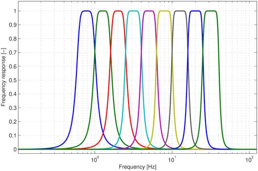
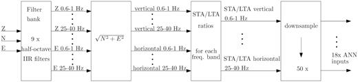
The inputs of the neurons are STA/LTA ratios of seismic traces in different frequency bands. We decompose each of the three components of velocity record (Z, vertical; N, north; E, east) in narrow-band signals by a filter bank of nine half-octave filters from 0.6 to 40 Hz (frequency response of the filters is in Fig. 4), then we combine horizontal components together with computing size of horizontal resultant. The processing scheme is shown in Fig. 5. In the next step we compute STA/LTA ratios and downsample the resulting signal. The original sample rate is then decimated to 5 Hz which is a compromise between the acceptable computational load and a good separation of individual waves.
4.2 Training and tests
For detection of local seismic events we need to emphasize the importance of event detection output right after S-wave onset. This is achieved by a much higher value of η1 near the S-wave arrival (Fig. 6c). After testing (for details and test performed see Doubravová et al.2016) we chose the most important point called LIWE to be 100.
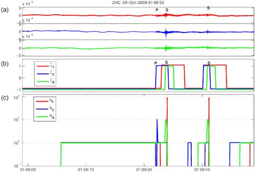
Learning example for two consecutive events. First one is stronger with manual reading of both, P- and S-phase, the latter one has S-wave reading only; (a) seismic traces from top vertical, north, east component of the ZHC station from 2008 October 8, (b) expected outputs, (c) learning coefficient function in logarithmic scale.5
During the training of the individual stations we achieved a good number of true positive rate (TPR) and true negative rate (TNR) compared to manual readings (for the best trained SLRNN TPR = 99.8 per cent and TNR = 78 per cent; that means 22 per cent false alarms). We inspected the results manually and found some false alarms to be small events omitted by manual processing. Some of the stations failed to detect events due to higher noise on the site, due to radiation pattern of a particular event, or in case of masking the waveform by the coda of the previous event. The proposed solution to this imperfection was to make use of the whole network of stations together. The coincidence of event-like waveforms on several stations in the network is crucial for successful and reliable event detection.
5 MULTIPLE STATION DETECTION—COINCIDENCE
In order to reduce the number of false detections as well as the number of undetected events due to higher signal-to-noise ratio we search for detection on other stations in the network to confirm or discard the event detection. Fig. 7 depicts three component velocity record and corresponding detection output. The detection is set whenever the detection output exceeds a certain threshold. The yellow stripes denote seismic events and one can see there are detections also in between the event stripes.
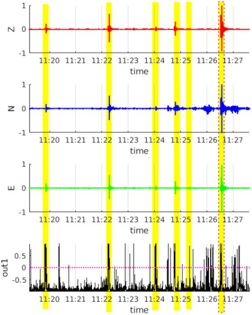
Example of the single-station detection. Seismogram from KLV station (2017 June 5, 11:20 to 11:27 UTC) filtered by BP of 1–40 Hz and detection output (always in range between −1 and 1). From the top: vertical, north, east component of velocity record, detection output of neural network. Yellow stripes denote seismic events (after coincidence), the strongest event marked by red dashed line is an event in SIL catalogue (ML= 0.9). The detection threshold (indicated by the purple dotted line) is exceeded even in between the events.
The proposed algorithm first scans all detections (detection output above zero) on all stations of the network and checks if there is a detection on a sufficient number of stations in the selected time window (we set it to 5 s with respect the size of the networks). In the next step we combine the detections together to make time intervals for events (see example in Fig. 8). As a result we define time segments containing useful information. Multiple overlapping events, especially during a swarm, lead to one time interval containing more events.
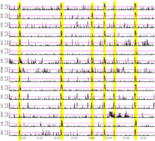
Example of the coincidence detection. Detection outputs of all 15 stations of REYKJANET, detection on at least six stations required. The same time segment as in Fig. 7.
The number of stations, which are needed to declare an event, is closely related to the number of false detections. Additionally, too many stations required might cause loss of weaker events. Fig. 9 shows an example of a coincidence of four and six stations and their comparison with the events detections performed manually (by the experienced interpreter). If we compare the detection results of the four- and six-station coincidence with the manual ones, it can be seen that the six-station coincidence detects all the manually identified events correctly while four-station coincidence detects also false events or events which are not interpretable (three cyan stripes which do not coincide with the yellow ones). Moreover, four station coincidence detecting more events which are merged if they overlap, produce longer time windows for events (broader stripes in Fig. 9). Two clearly separated event detections in six-station coincidence may become one longer event detection in case of four-station coincidence (note the end of the record where two yellow events become one longer cyan event). For both networks—WEBNET and REYKJANET—the coincidence of six stations seems to be the best option (see Tables 2 and 3 in Section 6.3).
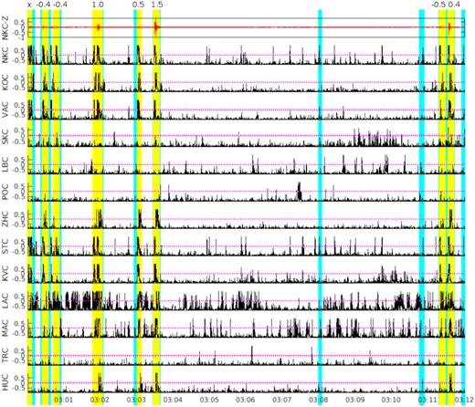
Example of the detection coincidence for four (cyan) and six (yellow) WEBNET stations. Red trace above is the vertical component of seismogram from NKC station from 2018 August 24 3:00–3:12 UTC. All events in yellow were also detected manually, magnitudes ML (from −0.5 to 1.5) are given above the yellow stripes. The first detected event in the seismogram is a multiple event consisting of several weak overlapping events, therefore the magnitude is not assigned (x sign is printed instead).
6 APPLICATION TO DATA FROM LOCAL SEISMIC NETWORKS
6.1 Evaluation of results
In an attempt to automatically compare manual catalogue to detections provided by the SLRNN we faced a problem with many weak events being missing in the manual catalogue correctly detected by the SLRNN. After all, the only reliable method to evaluate the correctness of each detection is to inspect it manually (Table 4). However, precise manual processing revealed also few weak events undetected by the SLRNN (usually with −1 < ML < −0.5). Our goal is to get complete catalogue down to ML = 0 for WEBNET and ML = 0.3 for REYKJANET. The smaller events will never be complete due to lower signal-to-noise ratio and are often unsuitable for further processing either.
In practice, we need to reduce the amount of data for further processing as much as possible, in other words to remove redundant data from the continuous recordings. On the other hand, if the selected time segment with a seismic event is few samples longer or shorter then it does not make a difference. In case of overlapping events during the seismic swarm, we joined detections together and therefore simply counting a number of detections does not correspond to the number of detected events. In case of a very sensitive network with low threshold or little coinciding stations, many swarm events blur into long time segment. The useful information is preserved but the reduction of data is less effective.
6.2 Application to REYKJANET
A potential ANN trained on the South-West Iceland data from REYKJANET poses quite a big problem because of the absence of complete catalogues/bulletins from the REYKJANET network which would be necessary to train the ANN. It is because of the REYKJANET recordings that have not been fully processed in detail like the WEBNET ones. To create relevant bulletins from the REYKJANET stations by manual processing of continuous recording would be extremely time-consuming, requiring an experienced specialist. Consequently, we mostly use the SIL catalogues provided by IMO for the REYKJANET-data analysis. But there are more detectable local events in the REYKJANET seismograms than those given in the SIL catalogues because REYKJANET is an evidently denser network (15 stations) than a regional network SIL including seven stations in the area concerned (Fig. 10). Therefore, an application of the neural network trained for the West Bohemia/Vogtland data (WEBNET) to data from South-West Iceland (REYKJANET) has been a challenging task. We took one of the best-performing SLRNNs as tested for WEBNET and applied it to the REYKJANET data. Since the deployment of the REYKJANET network in 2013, the seismicity on the Reykjanes Peninsula has typically been on a microearthquake level (magnitudes ML < 3) except two earthquake swarms in October 2013 (immediately after putting the REYKJANET stations into operation) with MLmax = 4.8 and in July 2017 with MLmax = 3.9 (MWmax = 4.1), and few weaker swarm-like episodes with magnitudes up to MLmax = 3.5. The swarms in October 2013 occurred on the tip of the peninsula out of the REYKJANET network. We analysed in detail the detection results for (i) four weak activities from the period 2014–2015, (ii) an intensive MLmax = 3.9 swarm of July 2017 and (iii) scattered background seismicity on the Reykjanes Peninsula in June 2017 (for basic data and locations of the analysed activities refer to Table 1 and Figs 10 and A3). The SIL catalogue is the primary reference for evaluation of the SLRNN-detection results for both (i) and (ii). Besides, we used a catalogue of the event detections produced by PePin automatic algorithm (Section 3) and Antelope software package (by Boulder Real Time Technologies, Ltd.) that were applied to the REYKJANET data of the activities given in (i), and a detailed bulletin of the 2017 swarm containing manual onset picks from all the REYKJANET stations.
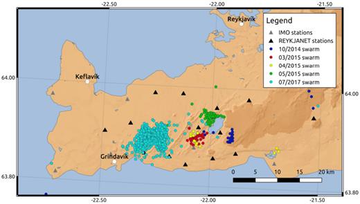
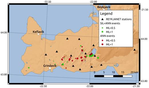
Map of Reykjanes Peninsula. Black triangles, REYKJANET stations; grey triangles, IMO stations; circles, epicentres of analysed earthquake activities. Blue circles, 2014 October 30–31 (MLmax = 2.8); red circles, 2015 March 31 (MLmax = 2.2); yellow circles, 2015 April 28–30 (MLmax = 1.6); green circles, 2015 May 29–30 (MLmax = 3.5); cyan circles: 2017 July 26–28 (MLmax = 3.9).
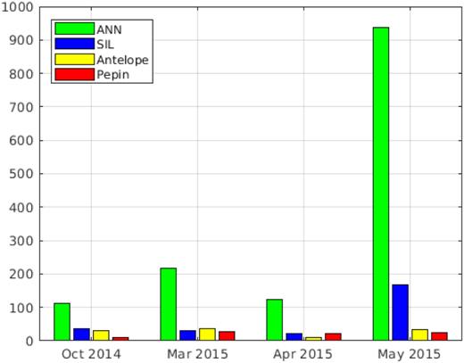
Number of events for all analysed Reykjanes activities.
| ANN | SIL | Antelope | PePin | Manual (above ML > 0) | |
|---|---|---|---|---|---|
| (i) 30–31 Oct 2014 | 112 | 37 | 30 | 9 | N/A |
| 31 Mar 2015 | 216 | 30 | 37 | 29 | N/A |
| 28–30 Apr 2015 | 125 | 23 | 9 | 23 | N/A |
| 29–30 May 2015 | 937 | 167 | 34 | 25 | N/A |
| (ii) 26 June 2017 | 124 | 56 | N/A | N/A | 281 |
| 11:00–12:00 | |||||
| (iii) 6–12 June 2017 | 184 | 34 | N/A | N/A | 64 |
(i) First, we compared the total number of detected events by the SIL processing, PePin algorithm, Antelope software and SLRNN (also denoted as ANN) in the individual weak activities. The Antelope automatic location procedure uses weighted STA/LTA phase detections (mainly P-wave phases are correctly picked). The PePin algorithm uses polarization analysis for event detection. In the first step the S-wave arrivals (which are often clearly polarized) are identified then they are associated with matching P-wave arrivals in the given time window, finally the event is localized. However, in case of a false event location (e.g. due to the incorrect association of the P- and S-wave arrivals) the event is omitted in the catalogue (for more information about the PePin detector see Fischer 2003). The comparison of the SIL, Antelope, PePin and ANN catalogues is depicted in Fig. 11. It is apparent the number of events detected by SIL, PePin and Antelope is comparable for all the activities, while the number of detected events by the SLRNN is about five times higher. We manually checked one of the activities with a reasonable number of events—the mini-swarm of the 2015 March 31. In total, 30 events have been listed in the SIL catalogue (MLmax = 2.2), 37 were located by Antelope and 28 by PePin.
Number of events in analysed microswarms on the Reykjanes Peninsula.
Inspecting the events manually, we found out none of the ‘catalogues’ (SIL, Antelope and PePin) to have been a complete subset of another one; each catalogue contained some unique events which were missing in the other two catalogues (see Fig. A1). The SLRNN detector provided 217 events including all the detected events given in the SIL, PePin and Antelope catalogues. Fig. A1 represents the comparison of detected/undetected events from each catalogue (SIL, PePin and Antelope) with those in the other two catalogues and with the SLRNN detections. By combining the SIL, PePin and Antelope catalogues we obtained 51 real events with minimum magnitudes ML ≈ 0. Our SLRNN detected all of them and in addition to that about three times more weak events. But many of the small detected events are unsuitable for further processing because locating of such events would be unreliable due to unclear P- and S-wave onsets. Nevertheless, Fig. 12 demonstrates that even the small events are true local seismic events, even they are on most of the stations buried in the noise. We believe that further automatic processing leading to a location would reject some of these event detections due to insufficient number of good quality phase readings.
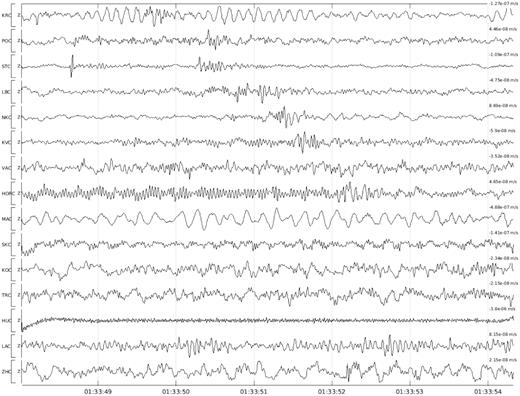
REYKJANET seismograms of one of the weakest events (ML = −0.6, roughly estimated) of 2015 March 31 detected by the SLRNN with six-station coincidence. 10 nearest stations (sorted by the epicentral distance) are shown. It is evident that the event is recognizable on the five nearest stations only, on the remaining stations its ‘useful’ signal is buried in noise. The event (its detection) is characterized by the maximum amplitude over all components of all stations in the whole detection time window (marked by dashed red line). Three component ground-motion velocity seismograms are filtered by BP of 1–40 Hz. The number above each trace gives the maximum amplitude of the ground-motion velocity in the displayed period.
Fig. A1 also point to the imperfect performance of the PePin algorithm because it missed two strongest and several other weaker events in the March 2015 activity (Fig. A1, top diagram in the figure). The PePin algorithm, which defines an event by associating the P- and S-wave phases, might have failed due to more complex waveforms resulting in the false association of the P- and S-wave phases (Section 3). Let us note that PePin has been routinely used in a near-real time processing of data from WEBNET.
(ii) A prominent earthquake swarm in July–August 2017 MLmax = 3.9 was fairly rapid. Most of the seismic moment released during 2 d from July 26 to 28 (Jakoubková 2018), more than 1500 ML > 0 events have been listed in the SIL catalogue for these days (Fig. A2). We concentrated on 1 hr of the swarm activity on July 26, from 11:00 to 12:00 UTC, that included the second strongest earthquake of the swarm (MLmax = 3.7). This segment contains both calm and turbulent phase of the swarm (Fig. A2). We performed detailed manual processing of the continuous seismograms with the assistance of an experienced expert who found 441 events in total out of which 281 were reliably located with magnitude above ML > 0. Then we compared the manually obtained events with detections provided by the SLRNN and with the list of events in SIL catalogue. There were 56 events in SIL catalogue and 124 event detections indicated by SLRNN (due to the turbulent nature of the swarm the detections often included more events). The results are shown in Figs 13 and A2. All of the manually picked events were correctly detected by the SLRNN and only one false SLRNN detection was found.
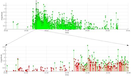
Magnitude-time distribution of the 2017 Reykjanes seismic swarm, only events with magnitude ML ≥ 0 are considered. Upper plot: the whole activity according to the SIL catalogue; lower plot: 1 hr segment around the second strongest shock of ML = 3.7 (2017 June 26, 11:00 to 12:00 UTC). Red points: events of the manually created REYKJANET catalogue which were missing in the SIL catalogue.
(iii) In order to prove the SLRNN ability to detect various local events on the whole Reykjanes Peninsula we selected a time segment containing scattered background non-swarm seismicity only (Fig. A3). We selected one week, 2017 June 6–12, where the seismic events included in the SIL catalogue were scattered in the whole area covered by the REYKJANET network. The SLRNN detected 183 events, 34 events of which had been listed in the SIL catalogue and no event present in SIL catalogue was missed. By manual processing of the waveforms we were able to confirm reliably 37 new events which we located and for which we estimated ML ranging from −0.5 to 1.3 (30 above ML= 0). Remaining 112 events were mostly unfit for location due to insufficient number of clear P- and S-wave onset picks or they were false alarms (or real events hidden in ambient noise).
6.3 Application to WEBNET
The WEBNET data are routinely processed by the PePin software (Fischer 2003) which provides good automatic locations in near-real time. The events located by PePin are then re-interpreted by manual processing (adding or refining picks, location by NLLoc with more precise velocity model, and in case of more significant activities some more advanced analyses). In order to get good location residuals, the PePin software is set up to use only eight nearest stations around the NK focal zone (the central part of the network) which contains more than 90 per cent of the total seismic moment released in the whole seismoactive area since 1991 (Jakoubková et al.2018). This unfortunately may result in omitting events outside the main focal zone. During November–December 2018 we compared in detail all events detected by the SLRNN (running in a pilot operation) with manual readings and with the PePin results. In this period the local seismicity was extremely low with maximum magnitude MLmax = 1.3. We took into account only events with magnitude above ML = −0.5, which resulted in 183 ones. The results of our analysis are summarized in Table 2 and Table 3 and displayed in Fig. 14. There are 106 events of ML > −0.5 successfully detected by both SLRNN and PePin (red circles in Fig. 14), 73 events were successfully detected by the SLRNN only (they are missing in the Pepin catalogue, yellow circles in Fig. 14), and four events missing in in the SLRNN list were successfully located by PePin (green circles in Fig. 14). It is worth mentioning that significant part of the undetected events by the PePin algorithm are located outside the main focal zone of Nový Kostel. Tables 2 and 3 provide more detailed statistics including the comparison of the detection results of the SLRNN with coincidence of six and four stations. The six-station coincidence, which we found to be an optimum for the West Bohemia/Vogtland earthquake-swarm region, results in omitting four events which were located both manually and by PePin; all four undetected events have magnitude MLmax ≈ −0.5. If we use four-station coincidence then all manually located events are successfully detected by the SLRNN but the number of event detections increase significantly. An example of one of the undetected events is given in Fig. A4. It is apparent that such small events may not be above noise level on sufficient number of stations.
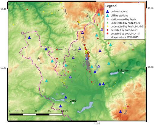
Detection results for local events during November and December 2018 in the map of West Bohemia/Vogtland. Blue triangles, online WEBNET stations; cyan triangles, offline WEBNET stations; pink triangles, stations used for near-real time data processing by the PePin algorithm; grey dots, epicentres of events in time period 1995–2015; red circles, events located manually and by PePin and also detected by SLRNN; yellow circles, events located manually and detected by SLRNN (not located by PePin); green circles, events located manually and by PePin (not detected by SLRNN). Diameter of circles is scaled according to local magnitude.
Number of events November–December 2018
| Data set | Number of events |
|---|---|
| Manual events | 317 |
| SLRNN detections—6 stations coincidence | 392 |
| SLRNN detections—4 stations coincidence | 840 |
| PePin events | 238 |
| Data set | Number of events |
|---|---|
| Manual events | 317 |
| SLRNN detections—6 stations coincidence | 392 |
| SLRNN detections—4 stations coincidence | 840 |
| PePin events | 238 |
Number of events compared to manual events for magnitude from ML > −0.5 and ML > 0, November–December 2018
| Manual events | Subset in SLRNN-6 | Subset in SLRNN-4 | Subset in PePin | |
|---|---|---|---|---|
| ML > −0.5 | 183 | 179 | 183 | 110 |
| ML > 0 | 43 | 43 | 43 | 27 |
| Manual events | Subset in SLRNN-6 | Subset in SLRNN-4 | Subset in PePin | |
|---|---|---|---|---|
| ML > −0.5 | 183 | 179 | 183 | 110 |
| ML > 0 | 43 | 43 | 43 | 27 |
7 DISCUSSION AND CONCLUSIONS
Processing of seismic records is a demanding task even for experts and interpreting continuous data from dense seismic networks is exhaustive and time-consuming. Therefore, it is desirable to hand over this job to machines. Automatic algorithms have served to replace manpower since many decades ago from triggered recording to automatic moment tensor solutions in near-real time. Studying earthquakes with low signal-to-noise ratio or overlapping events is still beyond the limits of automatic procedures although not negligible for many studies. We propose a seismic event detector based on ANNs to reduce the amount of data for further processing. The detector must be sensitive enough to recognize all the weak events with a manageable number of false alarms. The advantage of our neural network is the ability to recognize new events based on training examples (generalization capability) and very fast computation of the trained network. The weak point is the necessity to have very good manually prepared training data set. We showed that well-trained neural network can overcome this shortcoming and that a neural network trained on manually processed seismograms from WEBNET could be successfully applied to different local seismic network.
Following the approach of the interpreters, more stations in the network must be considered. This is an algorithm we call coincidence and setting up the parameters for coincidence we can lower the detection threshold at the cost of potentially more false alarms; or lower the number of false alarms at the cost of omitting weaker events. The result of such a process is a list of time periods containing a useful signal, irrespective to the complexity of seismograms. This way all the multiple and overlapping events remain in consideration for further processing.
The proposed neural network architecture—SLRNN with eight neurons—proved to be capable to detect local seismic events. Compared to automatic location algorithms based on searching for phase onsets the completeness achieved by detection is much higher. The reason is that the location algorithms must find sufficient number of correctly recognized onsets of seismic phases which is sometimes a challenging task even for trained experts. Additionally, the most effective detectors of S waves (as used among others in PePin) are based on polarization analysis, which tends to fail for weak events due to the high frequency content of the waveforms. If the number of phases found is not enough or they are incorrectly assigned, the event is usually irretrievably discarded. In case of detection we only try to recognize earthquake-like signals. This offers advantage for manual processing in terms there is no important event missing and the amount of data is reasonably reduced. For automatic location algorithms the reduction of data could be also beneficial and might increase their efficiency.
A coincidence of six stations for both networks—WEBNET and REYKJANET—seems to be optimal. Such configuration ensures detection of all important events and low completeness magnitude still preserving the number of false detections reasonable even for manual processing (Table 4). For further processing of detected events we recommend to use some amplitude- or power-based criteria to sort the events. We used simply the largest amplitude in the event period which is obviously not the best criteria. On the other hand even such an easy operation gives some guidelines. A weak event can have large amplitudes (for example if there is some disturbing signal present on some stations), but the strong local event will never be of small amplitude. This way we can exclude unimportant or negligible events from further processing by setting a suitable amplitude threshold.
Precision and recall calculated for analysed activities (only for those with manually processed events). The number of false positives (FP) is calculated with respect to a given magnitude threshold (ML > 0 or ML > −0.5) of reference manual events. For a lower magnitude threshold the number of FP decreases and the numbers of both TP and FN increase (compare line 4 and 6). REYKJANET (ii) activity is a piece of an intense swarm period, that is why there are no FPs and more detected events are often joined in one detection (as can be seen in Table 1). Denotation of data sets (i), (ii) and (iii) corresponds with that in Table 1. Abbreviation ‘6 sta’ or ‘4 sta’ denotes 6 or 4 station coincidence.
| Data set | TP | FP | FN | TPR (recall) | PPV (precision) |
|---|---|---|---|---|---|
| REYKJANET (i): 2015 Mar 31, ML > 0 | 51 | 165 | 0 | 1 | 0.236 |
| REYKJANET (ii), ML > 0 | 281 | 0 | 0 | 1 | 1 |
| REYKJANET (iii), ML > 0 | 184 | 120 | 0 | 1 | 0.605 |
| WEBNET 6 sta, ML > −0.5 | 179 | 213 | 4 | 0.978 | 0.457 |
| WEBNET 4 sta, ML > −0.5 | 183 | 657 | 0 | 1 | 0.206 |
| WEBNET 6 sta, ML > 0 | 43 | 349 | 0 | 1 | 0.11 |
| WEBNET 4 sta, ML > 0 | 43 | 797 | 0 | 1 | 0.051 |
Application to the REYKJANET data showed very good generalization ability of the neural network. Thanks to the generalization property of well-trained neural network we can use the same neural network for different region, or in case of West Bohemia for detection of events from different epicentral zones outside the main focal zone. We expect our trained neural network to perform similarly when being applied to any seismic activity with the frequency content similar to that used for training. The only difference in sensitivity is given by the background noise level, so we can expect lower completeness magnitude for the WEBNET data showing generally higher signal-to-noise ratio compared to the REYKJANET data. On the other hand, the proposed architecture could be possibly suitable for detection of regional or teleseismic events after new training and change of the input filtering.
In the near future there is a potential to use our neural network to pre-process data in project ICDP ‘Drilling the Eger Rift’ [more on https://www.icdp-online.org/projects/world/europe/eger/ or Dahm et al. (2013)]. An integral part of this project is the monitoring of seismic activity in West Bohemia using shallow boreholes equipped with broad-band seismometers supplemented with 3-D seismic arrays. The expected significantly larger amount of high-frequency microevents (with local magnitudes as low as ML ≈ −2) might be successfully detected by our SLRNN.
ACKNOWLEDGEMENTS
We thank Dr Gunnar B. Guðmundsson from the Icelandic Meteorological Office for providing SIL catalogues. Our special thanks are due to our colleague Alena Boušková for precise manual processing of the REYKJANET and WEBNET seismograms. We also thank the WEBNET team for technical care of the REYKJANET and WEBNET networks, particularly Jakub Klicpera. We are grateful to Dr Tomas Plenefisch and one anonymous reviewer for their thorough reviews and valuable suggestions that helped us to improve the paper substantially. We also thank the anonymous reviewer for corrections of English. Editor Prof. Huajian Yao devoted careful attention to this paper, we appreciate it. The work was accomplished within the Grant Project 18-05053S of the Grant Agency of the Czech Republic, ‘Physical processes related to swarm-like seismicity on the plate boundary in South Iceland and intraplate earthquake swarms in W-Bohemia/Vogtland’ and the project CzechGeo/EPOS-Sci (CZ.02.1.01/0.0/0.0/16_013/0001800, OP RDE) financed from the Operational Programme Research. The monitoring systems WEBNET and REYKJANET providing earthquake data received considerable support from the project LM2015079 CzechGeo/EPOS.
Footnotes
Reprinted from Computers & Geosciences, 93, Doubravová J., Wiszniowski J., Horálek J., Single layer recurrent neural network for detection of swarm-like earthquakes in W-Bohemia/Vogtland—the method, 138-149, Copyright (2016), with permission from Elsevier
Reprinted from Computers & Geosciences, 93, Doubravová J., Wiszniowski J., Horálek J., Single layer recurrent neural network for detection of swarm-like earthquakes in W-Bohemia/Vogtland—the method, 138-149, Copyright (2016), with permission from Elsevier
Reprinted from Computers & Geosciences, 93, Doubravová J., Wiszniowski J., Horálek J., Single layer recurrent neural network for detection of swarm-like earthquakes in W-Bohemia/Vogtland—the method, 138-149, Copyright (2016), with permission from Elsevier
Reprinted from Computers & Geosciences, 93, Doubravová J., Wiszniowski J., Horálek J., Single layer recurrent neural network for detection of swarm-like earthquakes in W-Bohemia/Vogtland—the method, 138-149, Copyright (2016), with permission from Elsevier
Reprinted from Computers & Geosciences, 93, Doubravová J., Wiszniowski J., Horálek J., Single layer recurrent neural network for detection of swarm-like earthquakes in W-Bohemia/Vogtland—the method, 138-149, Copyright (2016), with permission from Elsevier
REFERENCES
APPENDIX: ADDITIONAL FIGURES
Some more figures demonstrating (i) additional comparisons of events detected for selected activities that were recorded by REYKJANET (Figs A1 and A2), (ii) the distribution of the background seismicity on the Reykjanes peninsula (Fig. A3) and (iii) an example of one of four events undetected by the six-station coincidence for WEBNET (Fig. A4).
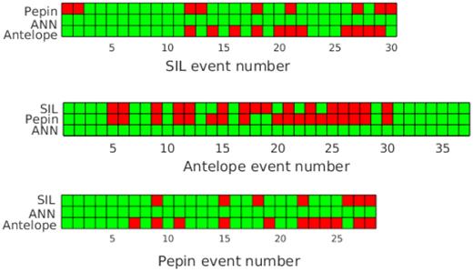
Detailed examination of the SLRNN detection results and the SIL, Antelope and PePin catalogues for mini-swarm of 2015 on the Reykjanes Peninsula. The diagrams represent the individual catalogues except SLRNN; from top to bottom: SIL, Antelope and PePin. Each column in the individual diagrams denotes a particular event in the respective catalogue (thus the number of columns in each diagram equals to the number of events in the catalogue). The events in the SIL and PePin diagrams are ordered according to magnitudes ML given in the SIL and PePin catalogues from the strongest (on the left) to the weakest one (on the right); the events in the Antelope diagram are sorted according to the origin time. The rows in the diagrams denote events which are included (green cells)/missing (red cells) in the remaining three catalogues (indicated on the right). The SLRNN diagram is not presented because a total of 217 events are detected by our SLRNN including all the events given in the SIL, Antelope and PePin catalogues. Note that the each catalogue (SIL, Antelope and PePin) contains some events detected only by ANN and missed in the other two catalogues.
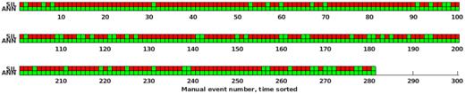
Comparison of the SLRNN detection results with the SIL and manual REYKJANET catalogue for 1 hr period of a larger 2017 swarm on the Reykjanes Peninsula. High rate seismicity in the time window of 2017 June 26, 11:00 to 12:00 UT, is examined. The diagram represents a comparison of the SLRNN results and SIL catalogue with the REYKJANET catalogue (281 ML > 0 events) created manually by an experienced interpreter. For more information on the diagram structure refer to the caption of Fig. A1. The events are sorted according to the origin time.
Examination of the SLRNN detections of background seismicity on the Reykjanes Peninsula in the period 2017 June 6–12. All 34 events listed in the SIL catalogue (green circles) are successfully detected by the SLRNN. Another 37 events (red circles) detected by the SLRNN are located using manual picks of the P- and S-wave onsets. 112 more event detections indicated by the SLRNN are the events unfit for location due to lack of reliable P- and S-wave arrival times or false alarms in some cases.
WEBNET seismograms of the local event (2008 November 14) undetected by SLRNN with the six-station coincidence. Manually estimated magnitude ML = −0.5. Only vertical components of the ground-motion velocity (BP 1–40 Hz applied) are displayed. Stations are sorted by epicentral distance (top trace corresponds to the nearest station).
