


Abstract
It has been shown on several tokamaks that application of a resonant magnetic perturbation (RMP) field to the plasma can lead to suppression or mitigation of edge-localized mode (ELM) instabilities. Due to the rotation of the plasma in the RMP field reference system, currents are induced on resonant surfaces within the plasma, consequently screening the original perturbation. In this work, the extensive set of 104 saddle loops installed on the COMPASS tokamak is utilized to measure the plasma response field for two n = 2 RMP configurations of different poloidal mode m spectra. It is shown that spatially the response field is in opposite phase to the original perturbation, and that the poloidal profile of the measured response field does not depend on the poloidal profile of the applied RMP. Simulations of the plasma response by the linear MHD code MARS-F (Liu et al 2000 Phys. Plasmas 7 3681) reveal that both of the studied RMP configurations are well screened by the plasma. Comparison of measured plasma response field with the simulated one shows a good agreement across the majority of poloidal angles, with the exception of the midplane low-field side area, where discrepancy is seen.
Export citation and abstract BibTeX RIS
1. Introduction
During tokamak operation in high energy confinement mode (H-mode), the plasma experiences periodic relaxations of its edge gradient in the pedestal region which are known as edge-localized modes (ELMs). ELMs carry the energy of bulk plasma to the tokamak wall. The unmitigated type I ELMs are a major concern for operation of the ITER device, since the energy they carry is sufficient to damage the first wall and the plasma divertor [1]. Recent work [2] offers a comprehensive review of investigated type I ELM mitigation techniques, namely high-velocity injection of frozen deuterium pellets into the plasma [3], fast movement of plasma position [4] and the non-axisymmetric perturbation of plasma equilibrium by radial field generated by resonant magnetic perturbation (RMP) coils [5].
Successful mitigation or suppression of the type I ELMs by RMP has already been demonstrated on a number of devices [6–9]. However, the exact physical mechanism of the mitigation is not yet fully understood and therefore extensive dedicated experimental effort is supported by modelling of RMP effects on the plasma with a variety of numerical codes (reviewed in [10]). One of the leading theories of plasma response to the RMP (supported by recent observations in [11]) states that when the hot conducting plasma is rotating in the reference frame connected with the RMP field, the screening currents are generated on corresponding resonant magnetic surfaces.
The present work compares experimental observations of the RMP plasma response on the COMPASS tokamak with the model based on the theory above. This paper is organized as follows: section 2 introduces the COMPASS system for RMP field generation as well as the magnetic diagnostics used to measure the plasma response to the RMP. Subsequently, section 3 provides the measured plasma RMP response for two studied RMP field configurations. In section 4 results are presented of the modelling of plasma RMP response by a linear MHD code MARS-F [12]. The spectra of generated perturbations mapped for the respective plasma equilibria are shown and the effect of plasma is discussed. In the last part of the paper in section 5, the measured and the modelled plasma responses are compared with each other, with similarities and differences discussed. The work is then summarized, and future work outlined, in section 6.
2. Experimental arrangement
2.1. RMP field generation in the COMPASS tokamak
The COMPASS tokamak is a compact-sized (R = 0.56 m, a = 0.2 m) experimental device of an ITER-like cross section, operated in a diverted plasma regime [13] (for more information about the discharge parameters used in this work, see section 4.2). Its RMP coil system consists of a series of independent ex-vessel conductors that cover the whole vacuum chamber and can be connected into a variable saddle coil configuration [14]. This offers a unique variability of the poloidal mode number m spectrum of the generated RMP. The two specific RMP configurations investigated in this work are depicted in figures 1(a) and (b) (plots were made using ERGOS code [15, 16]) and are referred to as on+off-midplane configuration and off-midplane configuration, respectively. All coils are single-turned, with the off-midplane coils being of even parity, while the midplane coils are of opposite polarity to them. Toroidally, the windings cover tokamak quadrants, generating an RMP field with toroidal mode number n = 1 and 2. In this work, the n = 2 field is used, since n = 1 field is more prone to causing mode locking of magnetic islands that are typically present in the plasma [14]. The spectrograms of the RMP field for magnetic equilibria studied in this work, generated by the on+off-midplane and off-midplane coil configuration are depicted in figures 7(a) and (b), respectively.
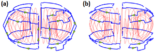
Figure 1. COMPASS RMP coil configurations used in this study. (a) On + off-midplane RMP configuration. (b) Off-midplane RMP configuration. Bold blue lines represent RMP windings; green arrows show direction of current; thin red lines represent plasma separatrix.
Download figure:
Standard image High-resolution imageThe RMP power supplies enable a single DC pulse per tokamak discharge of the same current magnitude in all of the RMP coils. The temporal evolution of the current waveform has the form of a trapezoid, with flat-top phase lasting several tens of milliseconds and current ramps from units to tens of milliseconds. The arrangement of the conductors generating the RMP uses two independent IGBT power supplies based on the design described in [17], but is capable of producing higher voltage.
2.2. Magnetic diagnostics of the RMP field
The tokamak chamber is covered by a set of 104 ex-vessel saddle loops, arranged into four quadrants (radially located below the RMP coil quadrants), as depicted in figure 2. Poloidal and toroidal angles (θ and ϕ, respectively) are shown for reference. Additionally, the radial location of the saddle loops with respect to the separatrix and the RMP coils is shown in figure 3.
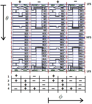
Figure 2. Scheme (not in scale) of 104 diagnostic saddle loops covering the chamber. Poloidal and toroidal angles θ and ϕ, respectively are shown, as well as low-field side LFS and high-field side HFS poloidal positions. Signs in the rows represent possible combinations of loop signals in order to obtain the n = 2 component, with the row in the top corresponding to large quadrant loops and the four bottom rows corresponding to octant loops.
Download figure:
Standard image High-resolution image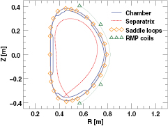
Figure 3. Poloidal cut of the COMPASS tokamak showing positions of separatrix (red dashed line), tokamak chamber and limiters (full blue lines), diagnostic saddle loop ends (orange diamonds) and RMP windings (green diamonds). Note that each saddle loop and RMP coil cover the whole poloidal surface between the two neighboring symbols.
Download figure:
Standard image High-resolution imageEach of the four quadrant sets consists of 22 large saddle loops covering the whole quadrant in toroidal direction (e.g. SE1-22), and of four smaller saddle loops on low-field side (LFS) that cover both octants per quadrant in two poloidal rows (e.g. SSE1-2 and ESE1-2). In order to cover the whole chamber, it is necessary for the loops to often adopt a more complex shape to avoid vacuum vessel ports. Moreover, the simplified scheme in figure 2 does not take into account that the loops cover a different poloidal range, as seen from the in-scale figure 3. Note, however, that the real loop geometry was taken into consideration in the evaluation of the magnetic field signals presented in this work.
The poloidal cut of the COMPASS tokamak in figure 3 depicts the relative positions of the tokamak chamber, diagnostic saddle loops, RMP coils and typical plasma separatrix. This illustrates that on the COMPASS tokamak:
- Plasma separatrix is located close to RMP coils.
- The RMP coils cover large poloidal sections—especially the midplane coil.
- Diagnostic saddle loops are of different size, with the largest area loops located on high field side (HFS) and the smallest area loops located on the top and the bottom part of the chamber.
- There is a sufficient number of saddle loops located underneath the RMP coils to provide good information about the spatial distribution of the RMP field.
By an appropriate combination of the signals of each poloidal row of the saddle loops across all four toroidal quadrants as illustrated by the signs in figure 2, namely:

the quantity Bn2 is obtained, which represents the n = 2 harmonic part of the normal component of the magnetic field. Since the quantities  represent normal components of the magnetic field measured by the loops of the respective quadrant (on the chosen row), the resultant Bn2 is averaged across both the toroidal and the poloidal span of the used loops. Given the unique diagnostic arrangement on the COMPASS tokamak, it is possible to measure Bn2 on up to 22 different poloidal positions. Moreover, with the two rows of small octant-covering saddle loops on LFS, there are four possible combinations for obtaining the Bn2 quantity (as shown in the bottom part of figure 2). Therefore, measurements on four different toroidal positions ϕ (corresponding to the center of the used octant or quadrant) are provided. Note that the combination of the small loops No. 2 is equivalent to combinations of the large quadrant loops and in fact is a linear combination of combinations No. 1 and No. 3 (just like combination No. 4 is). As the loops are located outside of the vessel, the high-frequency part of Bn2 is cut-off by skin effect at the frequency of approximately 40 kHz. However, this is of no concern since only the flat-top part of the DC RMP pulse is analyzed in this paper. The RMP current driven by the two independent power supplies is measured with a set of two Rogowski coils.
3. Measurement of plasma response to RMP field
To study the plasma response to the RMP field on COMPASS, two similar discharges with different RMP configurations were chosen. Namely, discharge #8078, with on+off-midplane RMP configuration, and discharge #9655, with off-midplane RMP configuration are considered and compared. Both discharges are ohmically heated, with plasma in diverted L-mode (lower single null configuration), i.e. in the regime that shows very good repeatability. The summary of their basic parameters is presented in table 1, with  representing the toroidal magnetic field, Iplasma the plasma current,
  the line-averaged electron density, q95 the safety factor and IRMP the current in RMP coils. Further information on profiles of the electron and ion temperatures and density are provided in figure 8 and discussed in section 4.2.
Table 1. Parameters of the analyzed discharges.
| Discharge number | 8078 | 9655 |
|---|---|---|
| RMP configuration | On+off-midplane | Off-midplane |
 (T) (T) |
1.14 | 1.14 |
| Iplasma (kA) | 230 | 230 |
 ( ( ) ) |
6.5 | 6.0 |
| q95 (—) | 3.6 | 3.5 |
| IRMP (kA) | 1.5 | 1.8 |
Due to its electro-magnetic nature, the plasma screening effect on the spectrum of generated RMP (see section 4 for details) can be detected by the magnetic diagnostic system of the saddle loops. During the RMP waveform, the measured Bn2 quantity from equation (1) is equivalent to

There, the original perturbation  was altered by the plasma response field
  . Taking into account the total mutual inductance
  between RMP coils and the corresponding saddle loop combination of poloidal position
  (measured by performing a vacuum shot with the RMP pulse of the given coil configuration), the original perturbation signal is obtained from:

 represents the total effective surface of the saddle loop row j and IRMP represents current in the RMP coils.
The resulting poloidal profile of the plasma response field  , as well as that of the original perturbation
  , is shown in figures 4(a) and (b) for on+off-midplane and off-midplane RMP configurations, respectively. Typically, the plasma RMP response is in opposite phase with respect to the vacuum field for the resonant harmonics of the RMP field spectrum, while being in-phase for some of the non-resonant components (see e.g. [18]). In figure 4 the phase between the overall
  and the
  seems to be opposite, which suggests that the screening effect might be dominant over the penetration. Measurements on TEXTOR [11, 19] indeed show that outside the plasma the overall response field of the screening-dominant regime is in opposite phase to the vacuum field and suggest that this phase difference might change as the RMP penetration advances. The validation of the latter effect on COMPASS is planned within the scope of future work.

Figure 4. Full poloidal angle θ profile of measured  (black triangles and the axis on the left) and
  (red diamonds and the axis on the right) components. (a) Discharge #8078 of on+off-midplane RMP. (b) Discharge #9655 of off-midplane RMP. Note that the missing data point in figure (a) is due to the malfunction of one of the detection loops.
Download figure:
Standard image High-resolution imageInterestingly, the strongest plasma response is observed in the LFS area of  , regardless of the RMP field configuration used. Additionally, in both configurations the ratio of
  under the bottom/top row RMP coils to the
  on the midplane is approximately the same, having a value of ≈0.5. Despite the fact that the vacuum field ratios are
  and
and  for on+off-midplane and off-midplane configurations, respectively. This implies that the midplane RMP coil row on COMPASS primarily affects the amplitude of the response, but not its poloidal profile. It is also observed that
  is approximately by an order of magnitude smaller than
  , which is further discussed in section 5.
Sketches of coil combinations in figure 2 show that Bn2 combinations are identical with respect to  shift and only opposite in polarity with respect to a
  shift. Therefore, the
  distribution of the
  can be illustrated by assigning the measured
  values to the whole quadrant and, afterwards, extended to the whole ϕ by using the symmetry described above. Moreover, the octant-covering saddles on LFS offer
  measurements on four different ϕ locations per quadrant. Thanks to the good spatial resolution of octant saddles, it can be seen from the
 plot in figure 5 that the plasma response field to both RMP configurations is, in fact, of helical nature, rather than being strictly in opposite phase to the imposed RMP field. This helical character is also further discussed in section 5, with respect to the modelling.
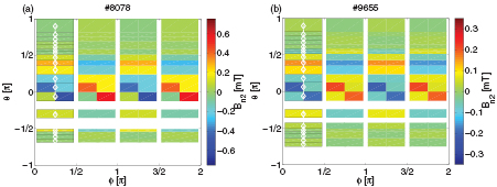
Figure 5. Visualization of the  profile of
  as measured by the saddle loops (taking their real dimensions into account). (a) On+off-midplane configuration of discharge #8078. (b) Off-midplane configuration of discharge #9655. White line and symbols represent the positions of the data points in figure 4. The black line grid represents the extent of the diagnostic saddle loops.
Download figure:
Standard image High-resolution image4. Modelling of plasma response
4.1. MARS-F code and modelled perturbation
The plasma response to both RMP configurations was modelled using the linear resistive MHD code MARS-F [12]. This code solves the linearized single-fluid MHD equations, assuming that the resulting perturbation of plasma equilibrium remains small [20]. Essentially, the non-axisymmetric RMP perturbation is imposed on the axisymmetric plasma equilibrium and a forced eigenvalue problem of stability is solved [10].
The unperturbed magnetic equilibrium of both discharges is provided by the numerical code EFIT+ + [21, 22], with the local magnetic measurements, the total plasma current Iplasma and the toroidal magnetic field  used as inputs. In both cases, the chosen equilibrium corresponds to the temporal moment of 1164 ms, i.e. to the flat-top phase of the RMP current waveform. In addition, the cross-talk of the RMP field on the magnetic measurements used as the input for the equilibrium reconstruction was eliminated in the same manner as shown in equation (3). The magnetic equilibria were remapped to a straight field line coordinate system, using the equilibrium solver CHEASE [23], prior to being used as the input for the MARS-F code. However, since the code requires a finite, well-defined q(a), the plasma X-point was slightly smoothed in the process of re-mapping.
In the model the RMP coils are represented as toroidally aligned straight lines of finite poloidal width that carry a toroidal harmonic current ∼ (with n = 2 in this paper) [24]. This representation naturally differs from the real coil geometry, and thus the RMP field calculated by MARS-F was compared to the RMP field calculation by the Biot–Savart law-based ERGOS code [15, 16], which takes into account the real coil geometry. Specifically, the comparison between the RMP field components aligned with the pitch angle of the magnetic equilibrium of discharge #7454, generated by the on+off-midplane RMP configuration can be seen in figure 6. Since the difference stays below 8%, the MARS-F coil representation is considered satisfactory.

Figure 6. Amplitudes of the pitch-aligned (i.e. on positions where q = m/n is fulfilled) components of  for the calibration discharge #7454, using the on+off-midplane RMP configuration. Black triangles represent calculation by ERGOS code, using the real RMP coil geometry. Red diamonds represent the calculation by MARS-F, using the simplified RMP geometry.
Download figure:
Standard image High-resolution imageThe quantity describing the spectrum of the RMP field in this paper (and consequently also plotted in figure 6), is the normal field component [15]:
R0 represents the radial position of the magnetic axis with B0 being the toroidal field on this position.  , with the poloidal magnetic flux ψ normalized with respect to the magnetic axis flux
  and to the magnetic flux on the plasma separatrix
  .
.  (note that
  ). The quantity
  represents the perturbation due to the RMP coils and
  the magnetic equilibrium field. Note that
  corresponds to the definition used in the ERGOS code. While n = 2 is fixed for the applied perturbation field, numerous poloidal mode number m harmonics of variable radial distribution are present. The spectra of the two studied RMP configurations (for the given plasma equilibria) are shown in figure 7.
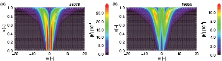
Figure 7. Spectrograms of the n = 2 vacuum RMP field  , calculated by MARS-F code. (a) On+off-midplane configuration of discharge #8078. (b) Off-midplane configuration of discharge #9655. White diamonds represent positions where condition q = m/n is fulfilled.
Download figure:
Standard image High-resolution imageFigure 7 shows the vacuum RMP field, i.e. without the effect of plasma. Comparison of figures 7(a) and (b) implies that the large midplane row RMP coils have a significant effect on the amplitude of the field, providing approximately half of the field magnitude. Distribution-wise, absence of the midplane coil row leads to the shift of the pronounced  harmonics from the plasma center to the edge regions, leading to much weaker magnitude of the generated RMP field on the midplane, with respect to the poloidal positions of the bottom/top coil row (see vacuum field distribution in figure 4 and discussion in section 3). The white diamond symbols in figure 7 show the location of the resonant surfaces satisfying the condition
  . Having them located close to the ridge of the spectrum, rather than its valleys implies good resonance between the plasma equilibrium and the vacuum RMP field at the COMPASS tokamak.
4.2. Modelled plasma response
In order to model the effect of plasma screening on the  spectrum, MARS-F needs to be provided with radial profiles of electron density ne, electron and ion temperatures Te and Ti and of toroidal plasma flow. On the COMPASS tokamak, the ne and Te profiles are measured by high-resolution Thomson scattering (HRTS, or TS in short) system [25–27], with spatial resolution up to 3 mm at the edge plasma, at the frequency of 60 Hz—see figure 8 for both studied discharges. The direct measurement of the Ti profile is not available presently. However, it is possible to obtain the profiles of Te and Ti from the METIS code simulations [28]. By overplotting all of the obtained temperature profiles in figures 8(b) and (d), one can see that there is a good agreement between the results by METIS and TS. Therefore, the Te and Ti profiles by METIS are used as the input for MARS-F in this paper.
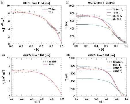
Figure 8. Plasma density and temperature profiles measured by TS and modelled by METIS. (a) ne profile of discharge #8078. (b) Te of discharge #8078 as measured by TS diagnostics, in comparison to Te and Ti provided by METIS simulation. (c) ne profile of discharge #9655 by TS diagnostics. (d) Te of discharge #9655 by TS and compared to Te and Ti provided by METIS simulation.
Download figure:
Standard image High-resolution imageSimilarly to Ti, the measurement of toroidal plasma flow is not available either. Although a well-established inter-machine empirical scaling relation exists for H-mode regimes [29], no such study was carried out for ohmic L-mode plasmas. However, on the Tokamak à Configuration Variable (TCV) an empirical relation for radial profile and magnitude of toroidal rotation velocity for ohmically heated L-mode discharges [30]
was found. We use this relation to obtain the toroidal plasma flow in this paper, taking into account that the TCV and COMPASS tokamaks are not too different in size ( m,
m,  m,
m,  m,
m,  m), as well as the similarity of the discharge parameters used to derive the relation (5) in [30] to the parameters shown in table 1. Therefore, the radial profile shapes of the toroidal plasma rotation frequency of the studied discharges are the same as those of Ti, with central
  kHz and
  kHz for discharges #8078 and #9655, respectively. This also yields central toroidal plasma rotation velocities of
  km s−1 for discharge #8078 and
  km s−1 for discharge #9655, which also agrees with typical
  magnitudes expected for ohmic L-mode tokamak plasmas (table 1 in [31]). Although the estimates from relation (5) developed for the TCV tokamak might not be entirely valid for COMPASS, in section 4.3 it is shown that the principal modelling results are fairly robust with respect to the possible
  uncertainty.
The resulting  spectrograms, with the plasma response included, are shown in figures 9(a) and (b) for the on+off-midplane configuration and the off-midplane configuration, respectively. By comparison with the spectra of the original vacuum perturbations in figure 7, it can be seen that the screening effect of plasma is strong in both studied discharges—the pitch-aligned components of the perturbation field, whose positions are depicted by the white diamonds, are having low magnitudes. Note also the shift of field spectrum distribution from the resonant components of positive m towards negative m values of the non-resonant components. The relation of the described RMP spectrum distortions with the
  quantity is further discussed in section 5.

Figure 9. Spectrograms of the total (including plasma response) n = 2 RMP field  , calculated by MARS-F code. (a) On+off-midplane configuration of discharge #8078. (b) Off-midplane configuration of discharge #9655. White diamonds represent positions where condition q = m/n is satisfied.
Download figure:
Standard image High-resolution imageAdditional insight into the nature of RMP screening on COMPASS is provided by figure 10. Here, the magnitudes of pitch-aligned components of  across the q = m/n resonant surfaces are shown—the original perturbation versus the perturbation with plasma response is included. First, comparison of the on+off-midplane configuration in figure 10(a) to the off-midplane configuration in figure 10(b) once again shows that the magnitude of generated resonant field is significantly lower in the absence of the large midplane coil row. Also, both plots show shallow RMP penetration into plasma, which takes place at approximately the same depth, regardless of the RMP configuration. Simulations with the quasi-linear MARS-Q code [20] are planned within the scope of future work, where the modelled penetration of the RMP is expected to reach deeper into the plasma [32].
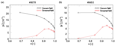
Figure 10. Amplitudes of the pitch-aligned components of RMP of the original vacuum perturbation (black triangles) and of the plasma-screened perturbation (red diamonds). (a) On+off-midplane configuration of discharge #8078. (b) Off-midplane configuration of discharge #9655.
Download figure:
Standard image High-resolution image4.3. Robustness with respect to plasma rotation
While it is safe to assume that the radial profile of toroidal plasma rotation is similar to that of Ti, the magnitude from the relation (5) might not entirely characterize the plasma rotation on the COMPASS tokamak. Therefore, an uncertainty by a factor of 2 was assumed and simulations with  and
and  were carried out. Specifically, central rotations
  kHz and
  kHz were assumed for discharge #8078 and
  kHz and
  kHz for discharge #9655, respectively.
The results of the simulations are shown in figure 11 on the pitch-aligned components of  , together with the original rotation simulations plotted for reference. It can be seen that within the tested frequency range, the effect on the magnitude of screened pitch-aligned components of
  is linear and small for both of the RMP configurations. Moreover, the depth of the penetration did not significantly change either. It is therefore concluded that the results are not significantly sensitive to the possible uncertainties in the determination of the
  .
.
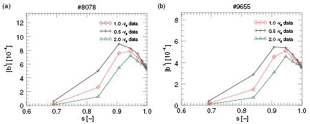
Figure 11. Amplitudes of the pitch-aligned components of the screened RMP field, for the plasma with original  (red diamonds), halved
  (black crosses) and double
  (green triangles). (a) On+off-midplane configuration of discharge #8078. (b) Off-midplane configuration of discharge #9655.
Download figure:
Standard image High-resolution image5. Comparison of the simulated  with the measurements

To compare the MARS-F simulated plasma response field to the experimentally determined quantity of  from section 3, a relevant quantity needs to be extracted from the simulation results. Specifically, the component of the total (with respect to m) magnetic field of n = 2 periodicity, radially located on the tokamak chamber and of normal direction to this surface is calculated from the
  spectrum for this purpose. The magnetic field component representing the plasma response is obtained using relation (2), with
  representing the vacuum perturbation field from section 4.1, and
  representing the screened perturbation field from section 4.2. Additionally, due to the different definitions of Bn2 quantities by MARS-F and relation (1), we normalized the MARS-F results by

The resulting modelled 
 profile is depicted in figures 12(a) and (b), for on+off-midplane and off-midplane RMP configuration, respectively. Comparison of these profiles with the measurements in figure 5, shows that the used model reproduces both the helical character of the
  , as well as its poloidal localization in the
  range. It should be noted, however, that the measured response in figure 5 and the simulated response in figure 12 are not entirely the same quantity as the former is averaged across the whole surface of a saddle loop. Therefore, the known
  dimensions of the detection saddle loops are used to average the modelled local
  field across the loop surfaces (see figure 12). The appropriate toroidal positioning of the loop mesh was validated by finding the best fit between the measured
  and the modelled one upon averaging. The relative position of the saddle loop mesh and
  generated by the both RMP coil configurations can be seen in figure 13. It should also be noted that, while for simplicity the loop system illustrated in figures 12 and 13 has no port-avoiding turns (e.g. seen in figure 2), they are in fact implemented in the averaging procedure.

Figure 12.  profile of
  as calculated by MARS-F. (a) On+off-midplane configuration of discharge #8078. (b) Off-midplane configuration of discharge #9655. The black lines represent the saddle loop grid, over which the averaging for figure 14 took place. Note that the depicted saddle loop scheme is simplified for clarity.
Download figure:
Standard image High-resolution image
Figure 13.  profile of
  as calculated by MARS-F, illustrating the relative position between the original RMP field and the averaging grid. (a) On+off-midplane configuration of discharge #8078. (b) Off-midplane configuration of discharge #9655.
Download figure:
Standard image High-resolution imageThe model-averaged and the measured  are compared in figures 14(a) and (b), for on+off-midplane and off-midplane configurations, respectively. Figure 14 shows good agreement between the linear MARS-F model and measurements of the plasma RMP response for both tested RMP field configurations across most of the poloidal angle θ. Linking this to the simulated strong plasma screening effects reported in section 4.2, together with the observations of spatial anti-phase of
  to
to  , it confirms that the measured
  is indeed expected to be an order below the original perturbation.

Figure 14. θ profile of  field, both measured by saddle loops (red diamonds) and modelled by MARS-F and averaged across the surface spanned by the saddle loops (blue triangles). (a) On+off-midplane configuration of discharge #8078. (b) Off-midplane configuration of discharge #9655.
Download figure:
Standard image High-resolution image
There is, however, a notable discrepancy between the simulated and measured  in the LFS area. Specifically, the measured LFS plasma response field is dominant over the one corresponding to the locations of the bottom and the top rows of the RMP coils (
 ) by approximately a factor of 2, as was mentioned in section 3. This is not observed in the simulated results and will be subject to investigation in future work, e.g. by using quasi-linear modelling with MARS-Q to take into account momentum transport and its effect on plasma screening [32], or by using more relevant profiles of toroidal plasma flow, obtained from the CXRS measurements [33].
6. Summary
Two configurations of the n = 2 RMP field on the COMPASS tokamak were introduced. They differ by the presence or absence of the large RMP coils on the midplane, in addition to the standard bottom and top coil rows of even parity. The RMP field was analyzed:
- By magnetic measurements using the extensive set of 104 saddle loops covering the whole tokamak vessel.
- By linear MHD simulations using the MARS-F code, based on the measured and simulated plasma profiles and equilibria.
In the experiment, it was observed that for both of the studied RMP configurations, the plasma response field of  is close to being in opposite phase to the original perturbation of
  as well as being approximately one order of magnitude below the
  . The shape of the plasma response field profile along θ was reported to be invariant to the inclusion of the large RMP coils at the midplane. The ratio between the
  magnitudes on the poloidal positions of
  (where the top and the bottom rows of the RMP coils are located) and the midplane
  magnitude, remains ≈0.5 across the studied RMP configurations, which implies that their perturbation eigenmode structure might be the same or very similar. The large midplane RMP coils have nevertheless a significant effect on the magnitude of the RMP field as a whole.
By modelling the RMP configurations with the MARS-F code, it was seen that there is a good resonance between the original, non-screened RMP and the chosen plasma equilibria. Similarly to the experimental observations, the midplane RMP coils' row was seen to have a significant effect on the magnitude of the perturbation as a whole. Simulations of the plasma response have revealed a strong screening effect of the plasma on the RMP spectra, consistent with the experimentally observed phase shift between  and
and  . Also, both the experiment and the model show that
  is of helical character in the
  plane. According to the linear model simulations, the penetration of the RMP into the COMPASS plasma is relatively shallow.
A good agreement between the  from the experiment and the model is reported across most of the θ angle, with an exception of the discrepancy on the LFS. The reason for this is currently under investigation and may be associated with the physics not taken into account by the linear model, or with the variation of the toroidal plasma flow profiles. Future endeavours in this specific area will thus include simulations by the quasilinear MHD code MARS-Q, more accurate measurements of the Ti and
  profiles by using CXRS, and attempts to directly measure the screening currents.
Acknowledgments
This work was supported by the Ministry of Education, Youth and Sports CR grant numbers 8D15001 and LM2015045, by the Czech Science Foundation grants GA14-35260S and GA16-24724S. This work has been carried out within the framework of the EUROfusion Consortium and has received funding from the Euratom research and training programme 2014–2018 under grant agreement number 633053 and from the RCUK Energy Programme, grant number EP/I501045. The views and opinions expressed herein do not necessarily reflect those of the European Commission.