
Development and Optimization of VGF-GaAs Crystal Growth Process Using Data Mining and Machine Learning Techniques


1
Leibniz-Institut für Kristallzüchtung, Max-Born-Str. 2, 12489 Berlin, Germany
2
Leibniz Institute for Catalysis, Albert-Einstein-Str. 29A, 18069 Rostock, Germany
3
Institute of Computer Science, Pod vodárenskou věží 2, 18207 Prague, Czech Republic
*
Author to whom correspondence should be addressed.
Crystals 2021, 11(10), 1218; https://doi.org/10.3390/cryst11101218
Submission received: 16 September 2021
/
Revised: 1 October 2021
/
Accepted: 5 October 2021
/
Published: 9 October 2021
(This article belongs to the Special Issue Artificial Intelligence for Crystal Growth and Characterization)
Abstract
:The aim of this study was to assess the ability of the various data mining and supervised machine learning techniques: correlation analysis, k-means clustering, principal component analysis and decision trees (regression and classification), to derive, optimize and understand the factors influencing VGF-GaAs growth. Training data were generated by Computational Fluid Dynamics (CFD) simulations and consisted of 130 datasets with 6 inputs (growth rate and power of 5 heaters) and 5 outputs (interface position and deflection, and temperatures at various positions in GaAs). Data mining results confirmed a good dispersion of the training data without the feasibility of a dimensionality reduction. Data clustering was observed in relation to the position of the crystallization front relative to the side heaters. Based on the statistical performance criteria and training results, decision trees identified the most decisive inputs and their ranges for a favorable interface shape and to keep GaAs temperature beyond limits for heavy arsenic evaporation. Decision trees are a recommendable machine learning technique with short training times and acceptable predictive accuracy based on small volume of CFD training data, capable of providing guidelines for understanding the crystal growth process, which is a prerequisite for the growth of low-cost, high-quality bulk crystals.
1. Introduction
The development and optimization of bulk crystal growth processes is a demanding task due to the multidisciplinarity of the phenomena associated with a phase change, numerous process parameters, challenging scale up and, in particular, the dynamic nature of the process with a considerable time delay [1].
Conventional experimental and CFD approaches to derive crystal growth process recipes are laborious, costly and time consuming. The common optimization approach described in [2] for process development based on the strategy of “inverse modeling” is limited to a small number of specific independent parameters (power of heaters) and a single optimization parameter interface deflection.
The recent tremendous success of artificial neural networks (ANN) [3] in detecting the complex patterns and relationships in non-linear static and dynamic data sets in related fields (e.g., [4]) has triggered feasibility studies on the application of ANN for the prediction of transport phenomena in crystal growth furnaces of semiconductors and optimization of growth parameters, inter alia [5,6,7,8,9,10,11,12,13,14,15,16,17,18]. In this case, the number and specification of the independent and optimization parameters are constrained only by the availability of the training data and not by the method. The process parameters could be numerous and various. Beyond ANN, there are also other various machine learning algorithms available. The guiding principles for the choice of the employed algorithm depend primarily on the quality of input data (e.g., data volume, noise, number of outliers, missing data etc.), type of output needed (regression, classification or clustering) and application constraints (trade-off between accuracy and interpretability). For example, a decision tree (DT) algorithm is successful in handling noisy data and outliers, artificial neural networks (ANN) in handling missing data and support vector machines (SVM) in the cases with low data volume. At the same time, some algorithms’ inter alia. random forests (ensembles of DTs) perform poorly out of the range of the training data.
It has been reported in the literature that ANNs outperform inter alia. decision trees, random forest, support vector machine, Gaussian processes, etc., concerning the accuracy of their predictions [19]. However, ANNs require much more data to be effective and therefore are computationally expensive. If an understanding of how each variable contributes to the prediction model is important, i.e., the interpretability of the predictions, then DTs are the better choice [20]. This is particularly important for the search for optimized growth conditions as, a priori, the variation of many parameters is necessary. If ‘‘sensitive parameters’’ have been identified, an optimization is easy and feasible [1].
In this study, the task of process understanding and optimization was approached by combining several data mining (DM) techniques: correlation analysis, k-means clustering and principal component analysis with machine learning (ML) methods: decision trees, i.e., regression (RT) and classification (DT) trees. DM integrates methods of exploratory statistical data analysis and ML methods. The above methods were chosen, while bulk crystal growth is generally viewed as a small data field where training data is expensive to produce or difficult to obtain from proprietary sources.
The final goal was to derive, optimize and understand the factors influencing the vertical gradient freeze (VGF) crystal growth process. Training data were generated by 2D CFD simulations.
All selected techniques were used to understand, quantify and rank influences of growth rate and the power of heaters on the interface deflection and maximal temperature in GaAs in order to grow low-cost high-quality crystals. The latter is characterized inter alia by a high growth velocity and by a flat solid/liquid interface.
As a process example, VGF-GaAs growth of 4-inch crystals was used. This process was selected due to the recent strong revival of interest in the III-V crystals as the crucial future materials for the next generation of wireless communications, i.e., for the microelectronic and optoelectronic devices in 5G and 6G technologies [21]. The success of the latter highly depends on the advancement in crystal manufacturing and obtained crystal quality. An additional reason was the axisymmetric nature of the VGF furnace [22] and fulfilled constraints for a quasi steady-state approach [23,24] that assures realistic high volume and high quality of training data. It is important to note that the applied methodology can be easily adopted by other materials and growth processes.
2. Models and Methodology
2.1. Generation of Training Data by CFD Modelling
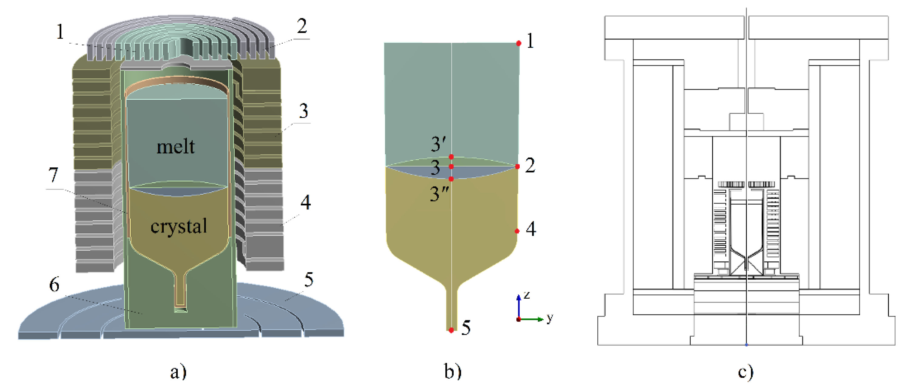
A simplified schema of the VGF-GaAs model is shown in Figure 1. The furnace geometry corresponded to a commercial furnace with five graphite resistance heaters. Top and side heaters were adopted for a generation of magnetic fields. In this study, no magnetic fields were considered. A cylindrical crucible made of pyrolytic boron nitride was loaded with ca. 9 kg of GaAs.
Due to the rotational symmetry, the furnace for the growth of 4 inches GaAs crystals was described by a 2D axisymmetric model. Governing equations for CFD modeling included equations of continuity, Navier Stokes with the Boussinesq approximation and energy equation (Equations (1)–(3)).
Weak buoyancy-driven melt convection [22] was described by the laminar flow model. All CFD simulations were performed using quasi steady-state (QSS) assumption. The QSS is justified if the characteristic time of the growth process is much larger than the characteristic time for heat transport, as is the case in VGF growth with weak buoyancy convection.
In the QSS approach, the latent heat released during crystal growth is included as an additional heat source at the crystallization front, and the growth rate is considered as a fixed input parameter. Along the solid/liquid interface, Stefan and isotherm conditions have to be satisfied (Equations (4) and (5)):
The GaAs material properties used in this study are given in [22]. The crystals were grown in Ar atmosphere under the pressure of 4 bar. The CFD simulations were performed using commercial code Crysmas.
For the generation of datasets for ML simulations, 130 combinations of heating power in 5 heaters in the range from 0–4 kW and growth rates in the range 0.1–5.4 mm/h were used as input parameters for the CFD simulations. From the obtained axisymmetric CFD results, the temperatures in the key monitoring points (MPs) in the melt and crystal (points marked 1 to 5 in a Figure 1b) and their corresponding coordinates were extracted for the ML training database. The interface deflection Δz was measured at the melt symmetry axis with respect to the three-phase junction (melt/crystal/crucible) and varied between detrimental concave (Δz > 0) and favorable slightly convex (Δz < 0) [22]. The origin of the coordinate system corresponded to the MP5. The GaAs crystals were grown in a positive z direction.
2.2. Data Mining
The DM techniques [25]: correlation analysis, k-means clustering and principal component analysis were used in this study before ML with the aim of assessing the quality of the training data and examining their relationships.
Correlation analysis is used to study the degree to which the variables are associated with each other, measured by the value of some kind of correlation coefficient, e.g., Pearson’s coefficient of correlation r given in Equation (6).
Two variables can be positively correlated (r > 0), when they are changing in the same direction (either increasing or decreasing simultaneously), negatively correlated (r < 0), when they are changing in the opposite direction, or can have a zero correlation (r = 0), when there is no relationship between the variables. In this study, a correlation plot with correlation coefficients for all input and output pairs of variables was prepared in order to examine their relationships.
Principal component analysis (PCA) is a data mining technique typically used to structure, simplify and illustrate large data sets by approximating a large number of statistical variables with a smaller number of linear combinations (the main components) that retain as large part of the overall variance as possible. A resulting PCA biplot can be used to visualize data dispersion, variables correlation and feasibility of dimensionality reduction by means of the PCA from the point of view of the retained variance. If the projections of two original variables into the 2-dim subspace of the first and second eigenvector form a small angle and at the same time have a very high proportion of the variance, the two variables are positively correlated. If the eigenvectors are orthogonal (close to 90°), they are not likely to be correlated. When they form a large angle (close to 180°), they are negatively correlated. If vectors have lengths completely different or the vectors are concentrated in the same quadrant of biplot, the distribution of data points has to be rethought.
K-means clustering is another data mining technique that aims to find groups in the data (clusters) based on feature similarity with the number of groups represented by the variable K. The goal is to divide vector (x1, x2, …, xn), into k (≤n) sets S = {S1, S2, …, Sk} so as to maximize the sum of squared deviations between points and the cluster center in the same cluster (Equation (7)):
2.3. Machine Learning
In this study, we selected the following DM/ML techniques: regression trees (RT) and classification trees (CT) [26] for the accurate prediction of VGF-GaAs growth recipes and easy understanding of the role of various process parameters. The RT is a type of DTs where the target variables are real numbers. The CT is other kind of DT where the target variables are labels of classes. Consequently, the RT is a type of supervised learning algorithm that can be used in regression problems, while the CT can be used in classification problems.
For both kinds of DT techniques, data comes in records of the form: (x, y) = (x1, x2, …, xk,y). The dependent variable y is the target variable that one is trying to model and predict. The vector x is composed of the inputs, x1, x2, …, xk.
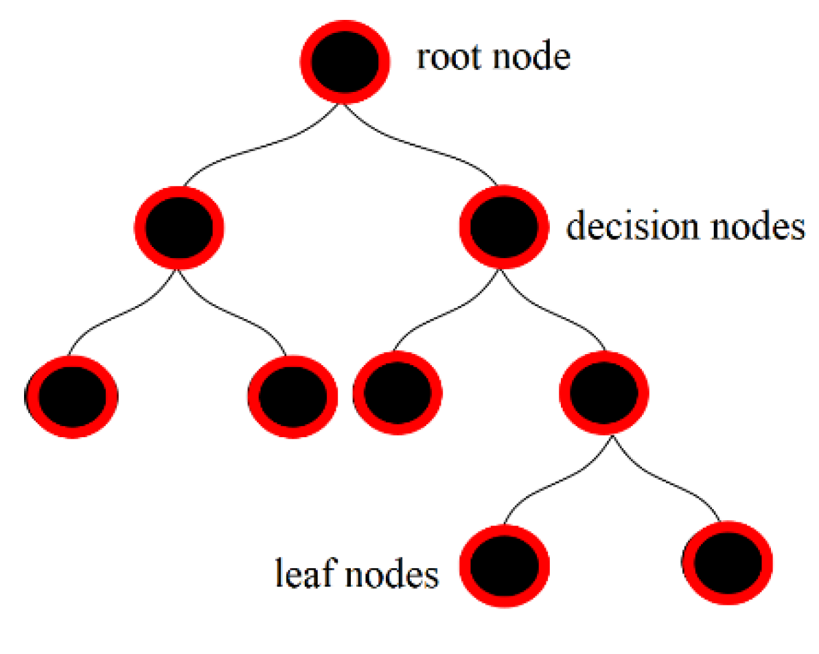
All DT algorithms have a tree structure (see Figure 2). Each node in the tree represents a variable from the input datasets, each branch a decision and each leaf at the end of a branch the corresponding output value. The decision process starts from the top root node (the entire dataset) downwards through the tree until a bottom leaf is reached, which contains the result (more homogeneous subsets of the initial dataset). At each node, the process of splitting and the path to be followed depends on the values yi of the output variable for the inputs xi in that node. More precisely, building a DT consists of recursive binary splitting of the training data, stopping only when each terminal node has fewer than some minimum number of datasets. In this study, that minimum leaf size was set to 4 and the maximum tree depth was set to 10.
For a regression tree, the splits are made in such a way that the sum of squared errors (SSE) with respect to the average values of the yi in the above subsets is minimal (Equation (8)).
Among all possible splits (S1,S2), a split (S1*,S2*) leading to the minimal SSE is chosen (Equation (9)).
First, this method is applied to the entire set of available input data, then to the resulting sets (S1*,S2*), etc. The splitting continues as long as necessary, forming a hierarchy of regions (tree) in the input space. The best tree is derived using cross-validation.
In RT analysis of process parameters affecting the crystal growth, the following six inputs were studied: x1 crystal growth rate, x2 and x3 heating power in the inner-top and outer-top heater, x4 and x5 heating power in the upper-side and lower-side heater and x6 heating power in the bottom heater.
The input variables were correlated with the two key outputs: y2-interface deflection and y3-temperature at GaAs free surface at the crucible rim (corresponding to MP3 and MP1 in Figure 1b, respectively).
In the CT analysis, the input variables were correlated with the output y2 to assess conditions for the growth of convex s/l interface, i.e., interface deflection y2 > 0. The same analysis can be performed for all other output variables.
The training data were identical to those used in DM analysis and consisted of the 130 (x,y) pairs. For assessing the effect of various inputs on specific output, regression and classification tree analysis and the comparison of mean output values were applied.
For both kinds of DT simulations, the commercial software Matlab® was used.
3. Results and Discussion
3.1. CFD Modeling
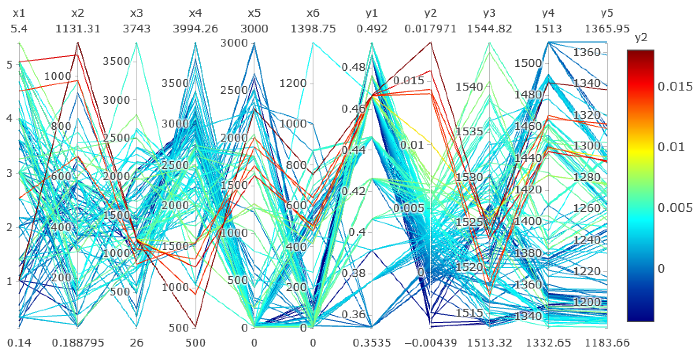
From the literature (e.g., [22] and beyond), it is known that typical temperature gradients in the GaAs melt and crystal in the industrial VGF processes are in the range of 2–10 K/cm and up to 15 K/cm, respectively. The crystal growth rate is typically in the range of 2–4 mm/h. The maximal temperature in the GaAs should not exceed 15 K above the melting temperature of GaAs (ca. T = 1528 K) in order to avoid a great loss of arsenic [2]. Guided by these facts, 130 process recipes were simulated and values of interface deflections, interface position and temperatures at the monitoring points at the GaAs seed bottom, end of cone and at the melt-free surface (Figure 1b) were collected. All data in the form of 11-dimensional datasets are shown in parallel coordinates in Figure 3. Each line in the plot corresponds to one data set (x1…x6, y1…y5). The generated database was used for DM/ML training and analysis.
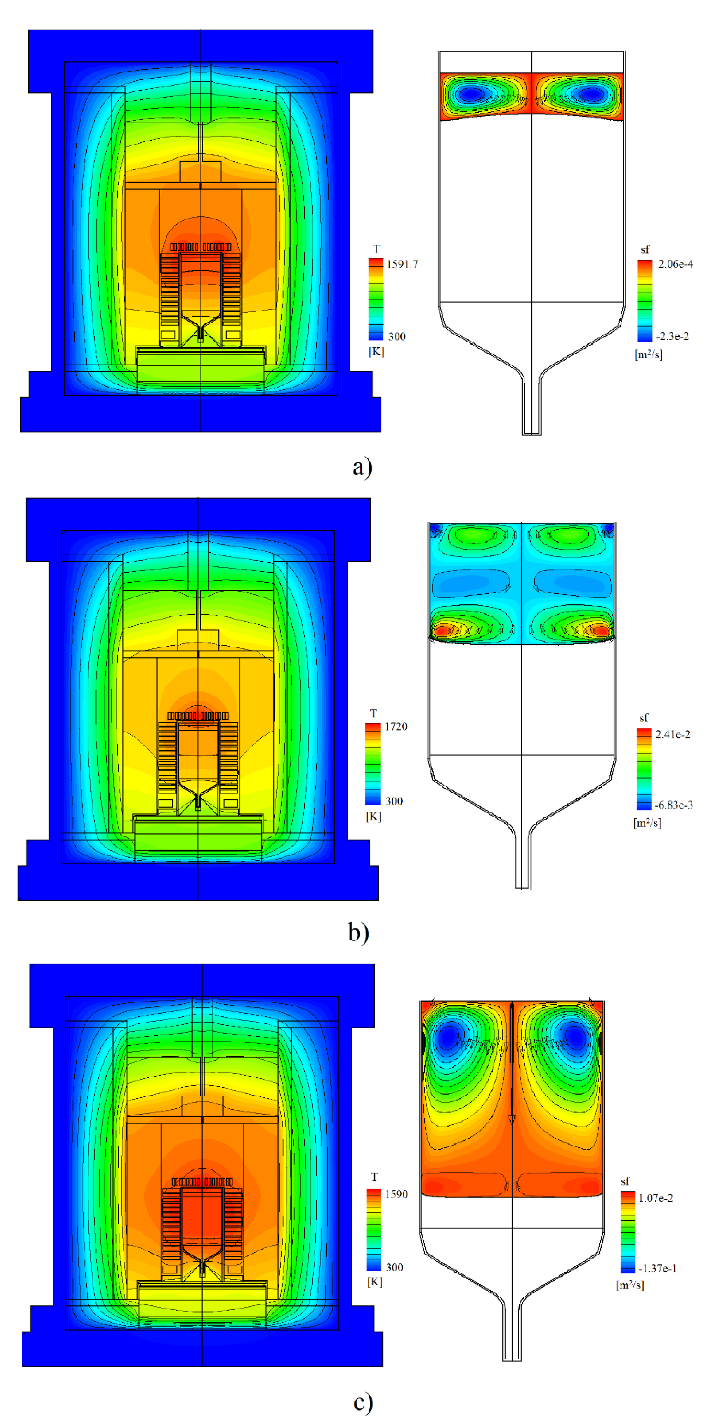
Examples of axisymmetric quasi steady-state CFD simulation results for buoyancy-driven flows in the form of temperature and stream function distributions in the VGF-furnace are shown in Figure 4. Due to the cylindrical geometry of the crucible, the melt flow was always toroidal, varying between multi-vortices (Figure 4b,c) and single vortex (Figure 4a) velocity distribution. Interface deflection varied between convex (Figure 4a), flat and concave (Figure 4b,c), depending on the used growth recipe.
As expected, our results confirmed the fact that generally favorable flat and/or a slightly convex s/l interface shape (y2 ≤ 0) was easier to obtain by lower growth rates x1 (Figure 3, blue lines). On the contrary, with an increase of the crystal growth rate (Figure 3, red lines), more latent heat is generated at the s/l interface and interface deflection turns toward concavity (y2 > 0).
Obviously, the search for the optimal VGF process parameters is a difficult task that requires advanced statistical methods.
3.2. Data Mining
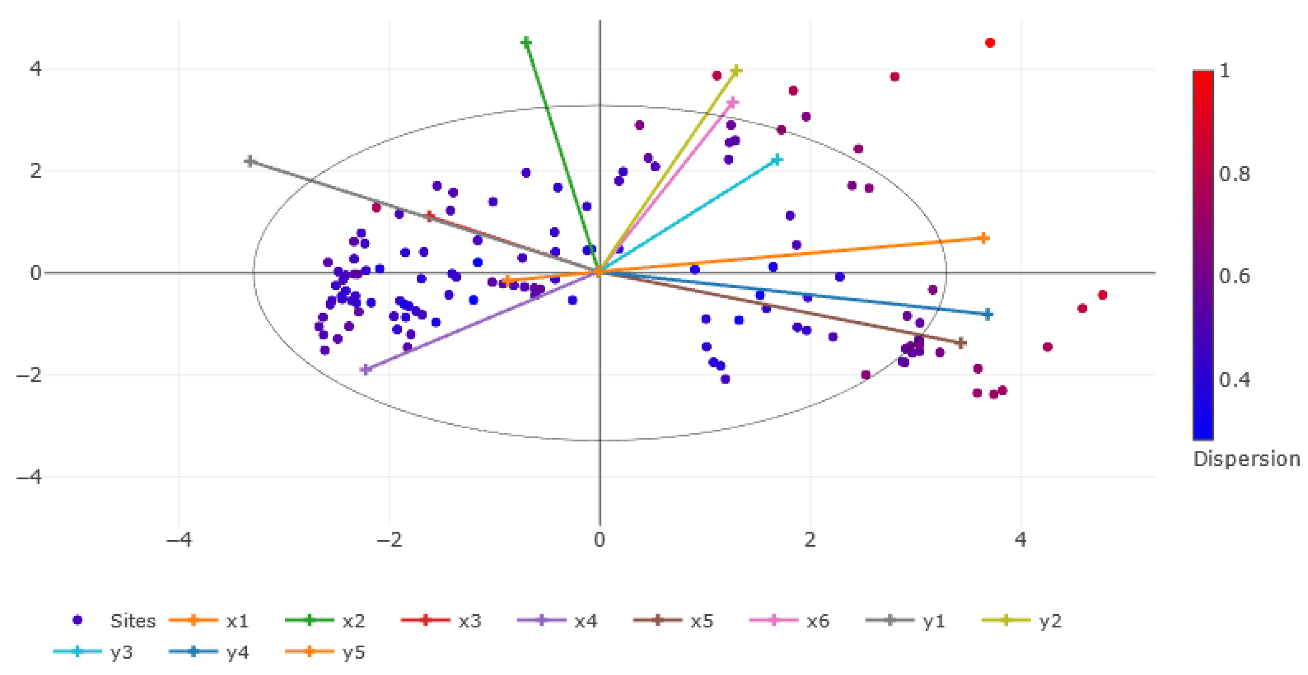
As mentioned before, PCA-biplot was used to visualize training data dispersion and variables correlation and to show the feasibility of dimensionality reduction without loss of information. The findings are given in Figure 5 and summarized below.
Since the two main components’ combined contribution to the variance is only 60.6%, i.e., not high enough, further discussion about the projections of original variables into the 2-dim subspace and corresponding correlations was not justified. However, the results showed that all vectors were present in all quadrants of the PCA-biplot and were of similar lengths, and therefore the distribution of points can be considered appropriate for further ML/DM analysis.
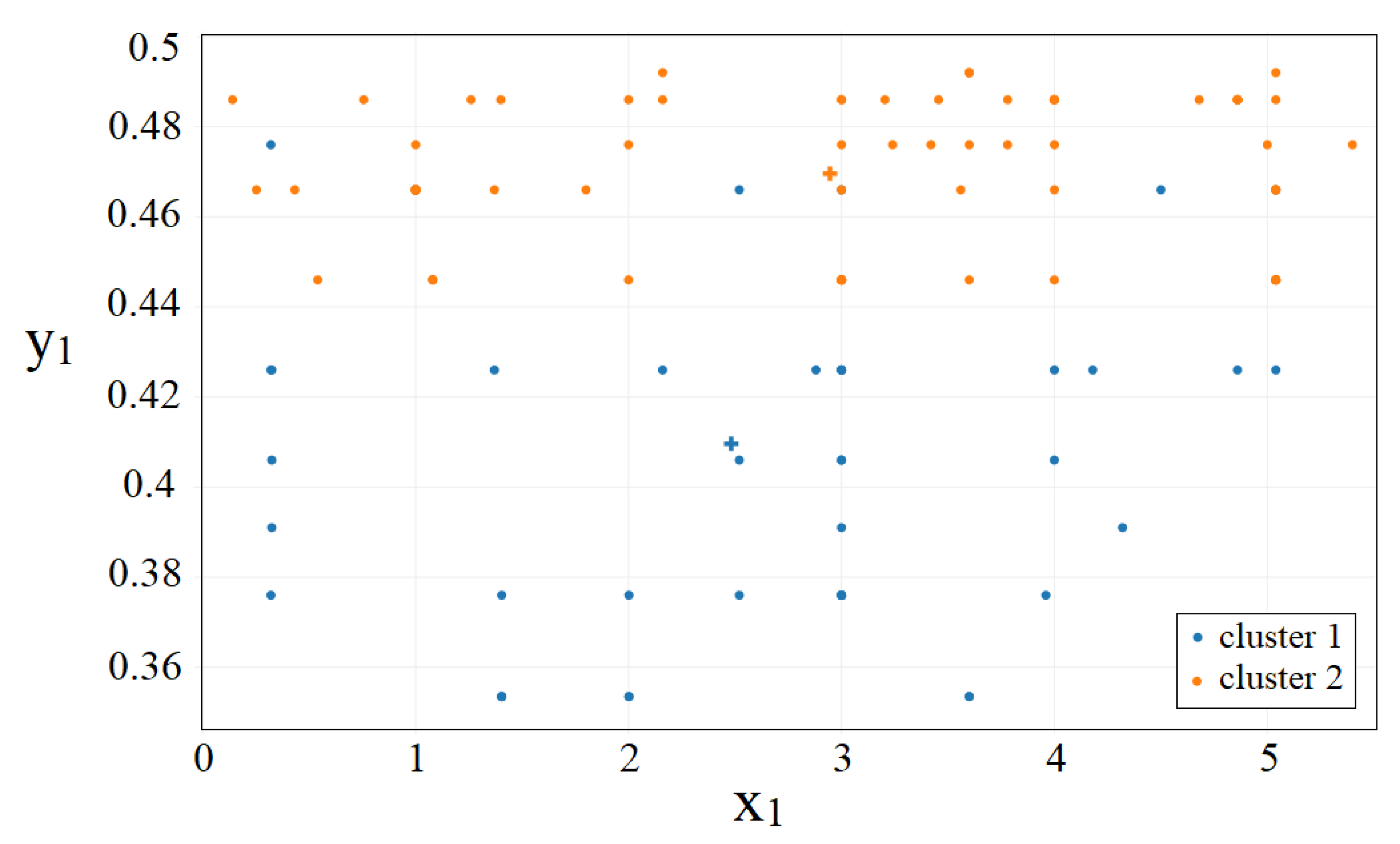
The k-means clustering method was applied to all 11 variables in this study. The k value varied from k = 2 to k = 10. The best clustering was observed for k = 2. Selected results for input x1 and output y1 are shown in Figure 6. These point out that, for all growth rates x1, there are 2 clusters of data with respect to the s/l interface position y1, i.e., data corresponding to the interface position y1 in the zone of influence of the upper side heater (z > 0.423 m) behave differently compared to the data in the zone of influence of the lower side heater (z < 0.423 m). This observation was used in further correlation analysis.
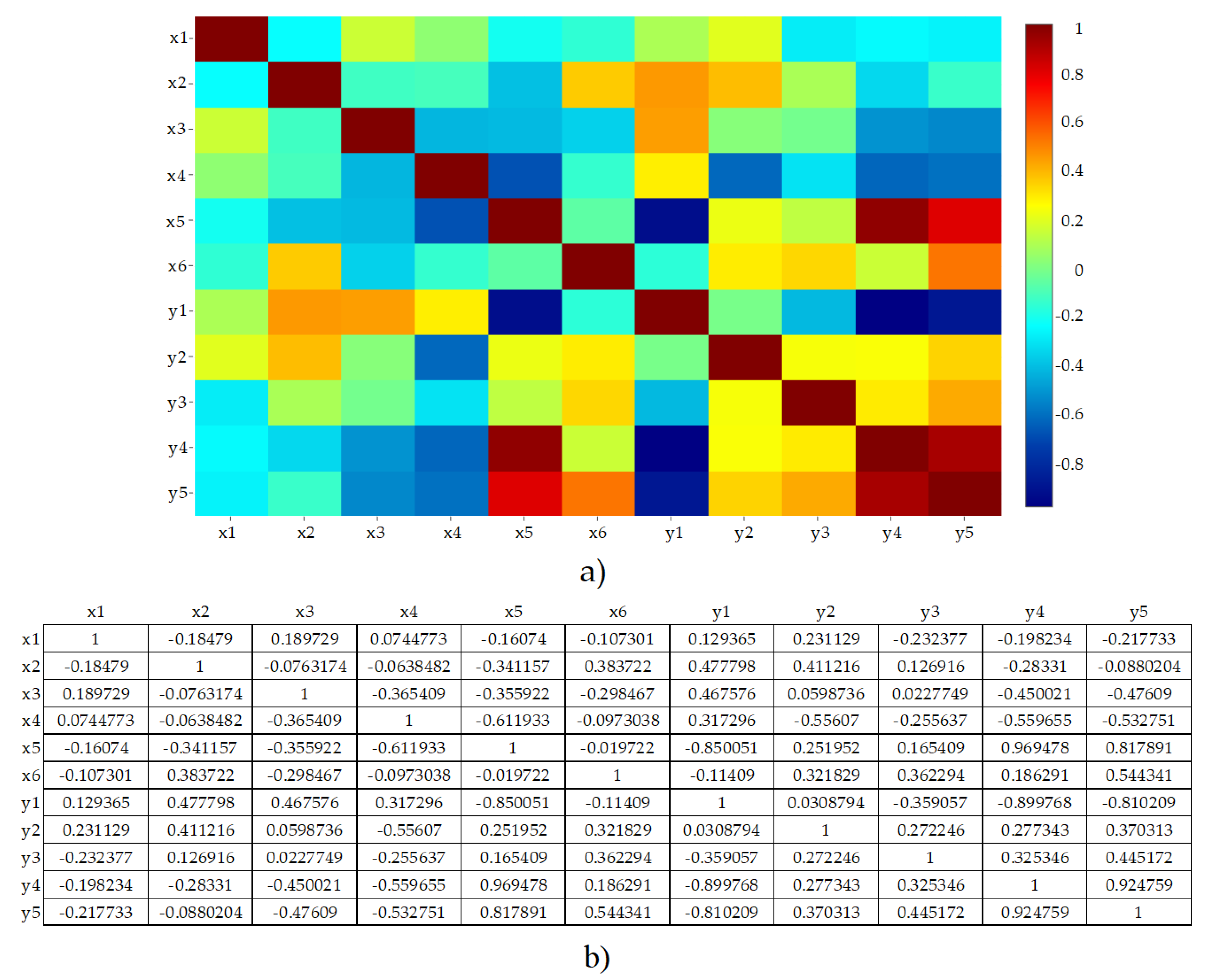
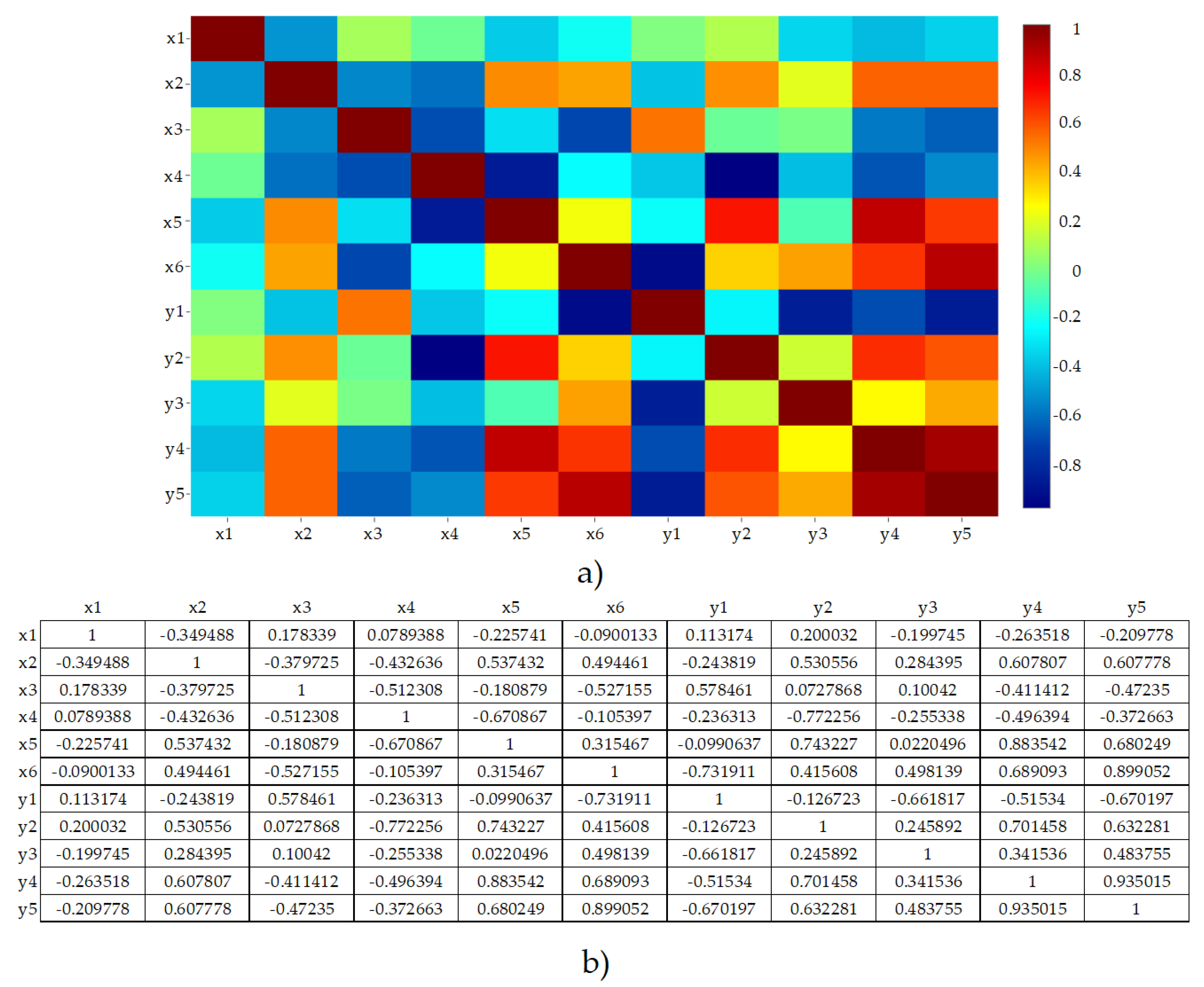
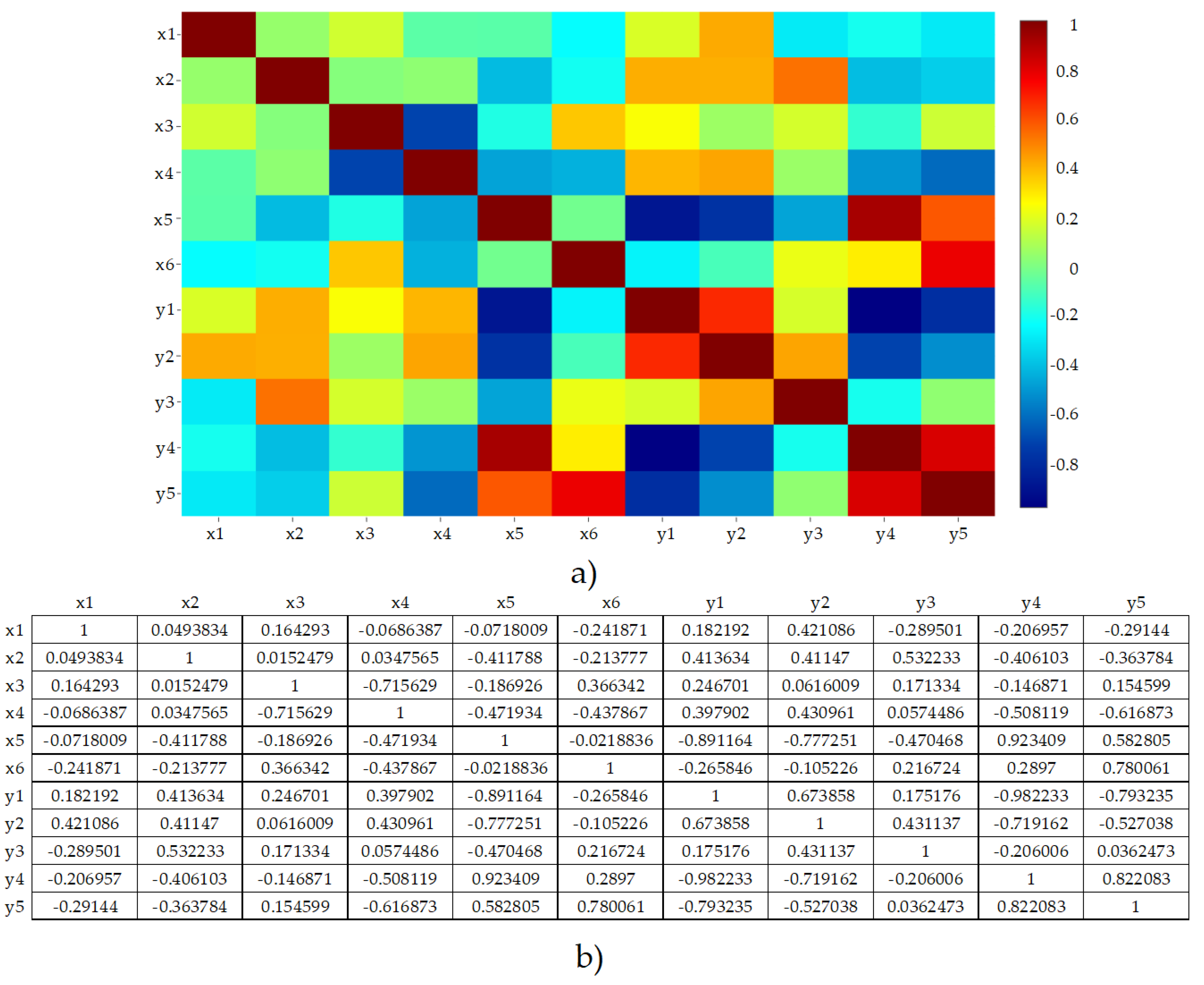
Results for the correlation plots for all data (whole crystallization process) for “lower” cluster 1 and “upper” cluster 2 are shown in Figure 7, Figure 8 and Figure 9, respectively.
From the analysis of the correlation coefficients for all data (Figure 7), it is possible to derive how inputs and outputs are correlated. The most pronounced correlation among inputs was observed by x4 and x5, i.e., by the power of the side heaters. Their correlation coefficient showed that they were weakly up to medium–strongly negatively correlated, with maximal value for rx4,x5 = −0.611. This result is in agreement with the nature of the VGF process, where the position of the crystallization front corresponds to a certain amount of the heating power and power distribution, and the growth rate determines the interface shape. Consequently, more power in the upper side heater implies less power in the lower side heater and vice versa. Concerning interface deflection y2, it is the most negative correlated by the increase of the power of upper side heater x4 (rx4,y2 = −0.556) and the most positive correlated by the increase of the power of top inner heater x2 (rx2,y2 = 0.411). Please note that in this study, convex interface deflection has a negative value (y2 < 0) and that a negative correlation is beneficial for the crystal quality.
For the GaAs temperature at the melt-free surface y3, the most pronounced negative correlation (weak with beneficial influence) had inputs: the power of upper side heater x4 and growth rate x1, since they decreased y3 value and therewith they limited severe As evaporation (rx4,y3 = −0.256, rx1,y3 = −0.232). The most pronounced positive correlation, but a detrimental influence on y3, had the power of the bottom heater x6 and the lower side heater x5 (rx6,y3 = 0.362, rx5,y3 = 0.165). These results can be explained if one recalls the typical heat transfer in the VGF growth, where heat is entering GaAs via melt and leaving via crystal periphery, in addition to the heat generated at the crystallization front. More heat coming from the crystallization front x1 and the upper side heater x4 means less heat coming from the top heaters x2 and x3 that are closer to the melt-free surface. More heat coming into the system from the x5 and x6 retards heat transfer out of the GaAs and consequently triggers the rise of the temperature y3.
From the analysis of the correlation coefficients for the “upper” data cluster 2 (Figure 8), interface deflection y2 was the strongest negative correlated by the power of upper side heater x4 (rx4,y2 = −0.772) and the strongest positive correlated by the power of lower side heater x5 (rx5,y2 = 0.743). The first result was identical to the result for the whole VGF process, i.e., for all data. The second result differed. It can be understood by remembering that the “upper” data cluster is related to the second half of the crystallization process with the crystallization front positioned above the lower side heater. In this case, x5 was bringing heat to the GaAs crystal that was harmful for y2.
For the temperature at the melt-free surface y3, the most pronounced negative and positive correlation were achieved by x4 (rx4,y3 = −0.255) and x6 (rx6,y3 = 0.498), respectively. These findings are similar to the case when data for the whole process are considered.
From the analysis of the correlation coefficients for the “lower” data cluster 1 (Figure 9), interface deflection y2 was influenced detrimentally in a similar strength by the x4, x1 and x2 (rx4,y2 = 0.431, rx1,y2 = 0.421, rx2,y2 = 0.411) and the most beneficially influenced by the power of lower side heater x5 (rx5,y2 = −0.777). The results are different in comparison to the result for the whole VGF process, i.e., for all data. This can be explained by the fact that the “lower” data cluster was related to the first half of the crystallization process, with the crystallization front positioned sidewise on the lower side heater and far away down from the top and upper side heaters.
For the temperature at the melt-free surface y3, the most beneficial and detrimental influence had x5 (rx5,y3 = −0.470) and x2 (rx2,y3 = 0.532), respectively. The greater heat was coming from the GaAs side periphery (x5), and less heat was coming from the top (x2) so that, consequently, y3 decreases.
Interestingly, the analysis of all correlation plots pointed out that the power of side heaters had a much stronger influence on the interface shape and maximal GaAs temperature than solely the crystal growth rate.
3.3. Decision Trees
As mentioned before, a successful VGF process is characterized inter alia by a flat crystallization front during the growth and constrained maximal temperatures in the melt to prevent strong arsenic evaporation/loss. The purpose of the DT analysis was to better understand the role of various process parameters and to identify their suitable values for the growth of high-quality crystals.
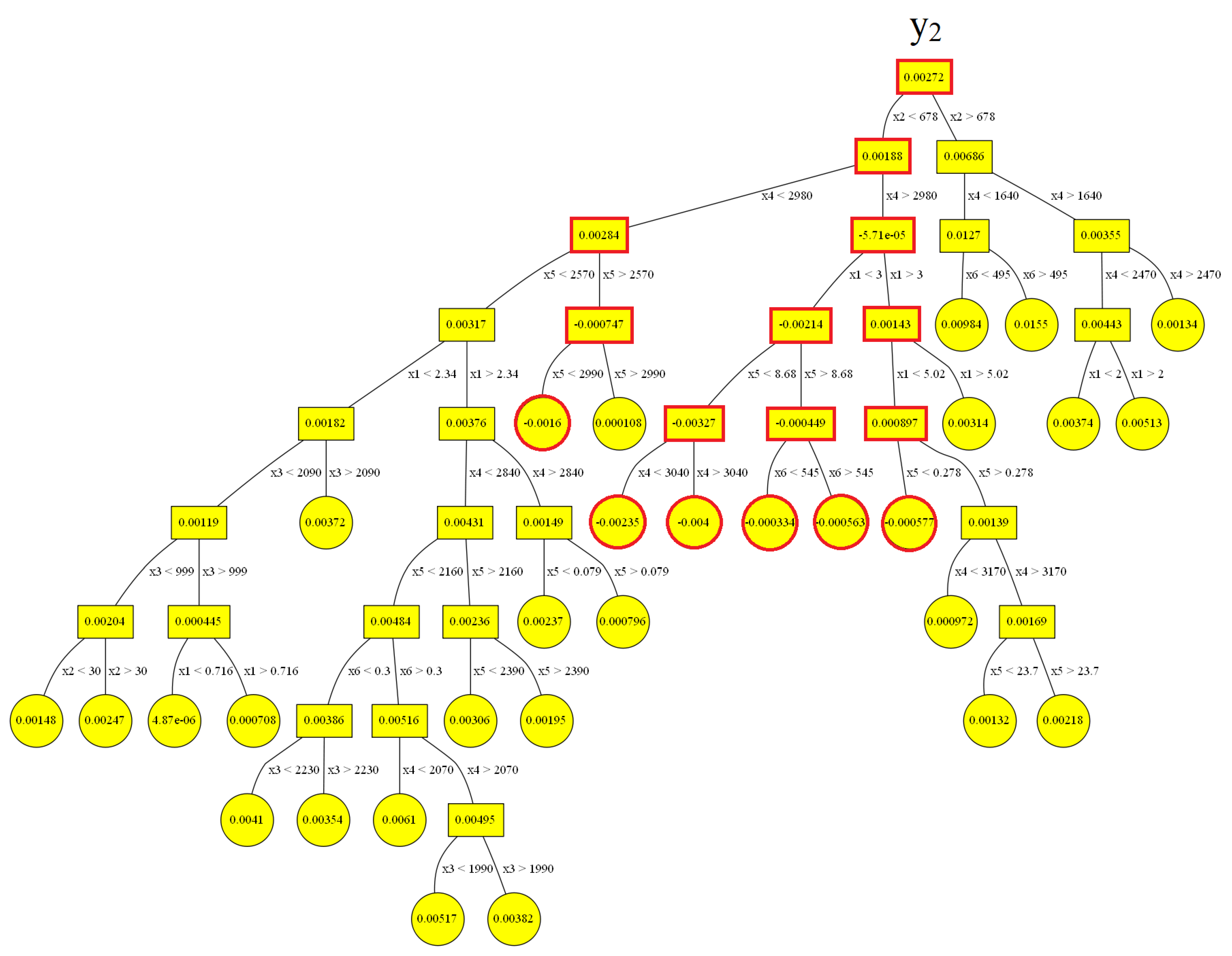
The most important DT results for both regression (RT) and classification trees (CT) are given in Figure 10, Figure 11 and Figure 12 with errors and summarized results in Table 1, Table 2, Table 3, Table 4 and Table 5. The errors are given in Table 1 and Table 4, in the form of the root mean square error RMSE corresponding to the nodes in the regression tree. The root node in the regression tree stands for the average value of the studied output among all data in the database. The path from the root to leaf states the influence of a certain input on the studied output, with the highest relevance at the top, decreasing downwards.
The resulting RT for interface deflection y2 is shown in Figure 10. It reveals x2, followed by x4 and x1, as the most decisive inputs for the favorable flat or slightly convex interface shape (interface deflection y1 ≤ 0, the branches marked red in the tree graph). Their significance decreases in the order mentioned above. The most decisive input is x2 (the heating power of the inner top heater) that has a deteriorating effect on the interface flattening, i.e., x2 should be below 678 W to strongly push y2 towards lower values (less concavity), i.e., from average y2 = 0.00272 m to average y2 = 0.00188 m. All decisive inputs and ranges of their optimal values that assure the VGF-GaAs growth with flat or slightly convex s/l interface (y2 ≤ 0 m), derived from RT analysis, are given in Table 2. For the fast growth of GaAs crystals (growth rate > 3 mm/h) with a flat or slightly convex interface, the process heat should be provided predominantly from the upper side heater (x4), while the bottom and lower side heater should be turned off. Moreover, the inner top heater should provide only a very limited amount of heat to the system. Obtained RT results are consistent with the findings from our correlation analysis, remembering the fact that the most influential input in RT doesn’t mean that its influence is necessarily beneficial for the variable y2. In the literature and among the crystal growers, there is a common opinion that the growth rate x1 has the strongest influence on the interface deflection (i.e., the higher the growth rate, the more generated latent heat at the crystallization front and consequently more concave s/l interface shape). Here obtained RT results do not refute the strong influence of x1. They mean only that other inputs outperformed the importance of x1 for y2.
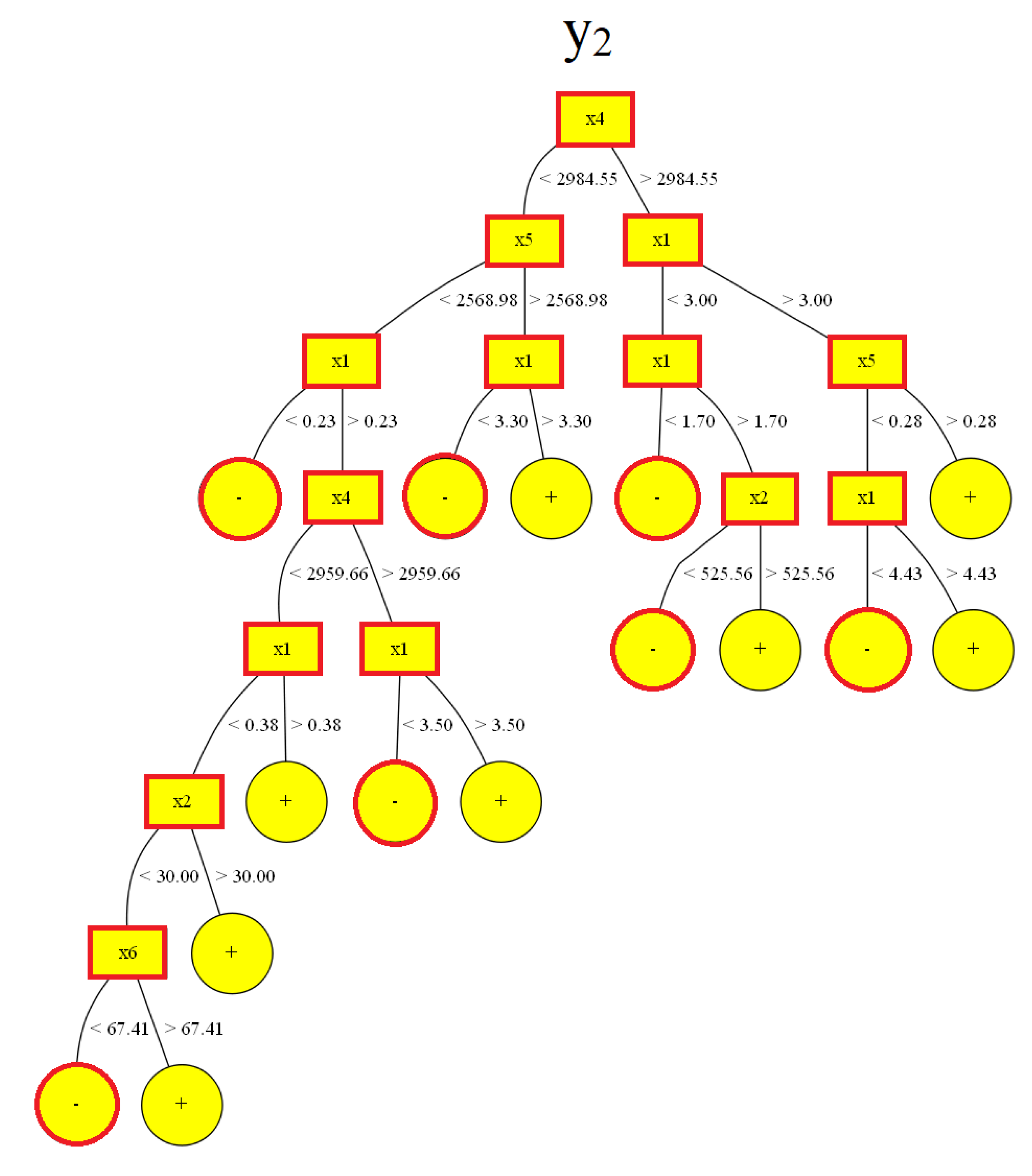
The same optimization task for y2 was solved using a classification tree. The target variable y2 consists further of real numbers and the classification task was performed associating these numbers with labels “+” for concave interface (y2 > 0) and “-“ for convex interface (y2 < 0). The CT results for interface deflection y2 are given in Figure 11, and the corresponding most influential inputs and their ranges for optimized growth are given in Table 3. Except for x3, all other inputs played some role. The most influential input for obtaining the convex interface was x4, followed by x1 and x5. As with the RT, the results showed that during the rapid growth of crystals with a slightly convex interface, the process heat should mainly be provided by the upper side heater (x4), while the lower side heater should be almost switched off.
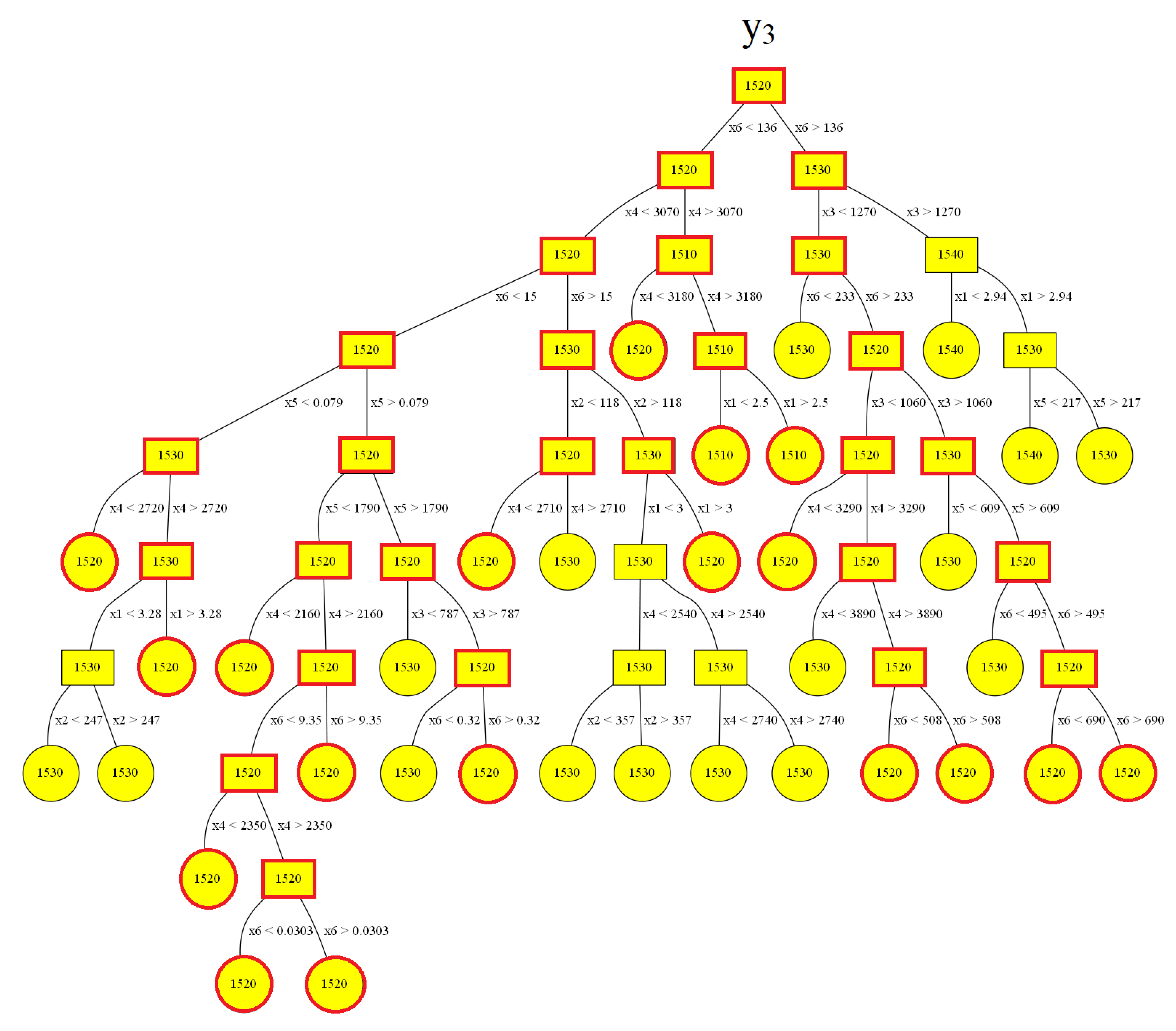
The resulting RT for the temperature at the melt top rim y3 is showed in Figure 12. The most decisive inputs and the range of their optimal values that prevent great loss of arsenic are given in Table 5. The data ranges correspond to the red marked branches in Figure 12.
The range of suitable parameters vary depending on the chosen maximal allowed temperature value, e.g. either 1520 K or even more conservative 1510 K. Still, all inputs x1-x6 played the role. The most influential input is x6, followed by x4. Other inputs are less important and appear at the lower position in the tree. The increase of the initial average value of y3 from 1520 K→1530 K after the first split, by the increase of the power of the bottom heater x6, showed their positive correlation, but detrimental influence. On the contrary, higher values of the x4 (x4 > 3070 W) after the second split caused the decrease of the average y3 values from 1520 K→1510 K and confirmed their negative correlation (with beneficial influence) observed by the correlation plots. As with the RT for y2, the results of RT analysis for y3 showed again that during the optimized rapid growth of crystals (x1 > 3.28 mm/h) without great loss of arsenic, the process heat should mainly be provided by the upper side heater (x4), while the lower side and bottom heaters (x5 and x6) should be almost switched off (Table 5).
In summary, our RT and CT analysis revealed the key process parameters, their importance and the ranges of their values for achieving beneficial conditions for the VGF-GaAs growth.
To compare the DM and ML techniques used here, it is important to note that the DM techniques measured the relationship between one pair of variables among the inputs and outputs (x1…x6, y1…y5), while ML/DT measured the relationships between all inputs and one output (x1,…x6, yi) and suggested the range of their optimal values. For the simultaneous optimization of all outputs in relation to all inputs, artificial neural networks are the best choice. The latter, however, is associated with a loss of interpretability, much higher computing times and a vast amount of training data, which is often difficult to come by.
4. Conclusions
This study demonstrated the capabilities of data mining and machine learning in smart derivation of the crystal growth recipes on the example of VGF-GaAs growth.
The data mining and machine learning techniques used were: correlation analysis, k-means clustering, principal component analysis and decision trees extract patterns and correlations among the raw process data. The decision trees, both regression and classification type, are an excellent choice if we need a machine learning model with short training times based on a low volume of CFD training data able to provide human-comprehensible results. The decision trees also provide ranges of process parameters (e.g., power of heaters and growth rate) where nearly-optimal values of the output variables (e.g., interface deflection or maximal temperature in GaAs) can be found.
The results of the correlation analysis, the k-means clustering and the principal component analysis showed the good scatter of the training data and the existing correlation between all variables, without the possibility of dimensionality reduction.
The regression trees predicted: (i) the most influential input to keep the GaAs temperature below the limits for high arsenic evaporation is the heating power in the bottom heater x6, followed by the heating power in the upper side heater x4; (ii) the most influential input for shaping the solid–liquid interface is the heating power of the inner top heater x2, followed by the heating power of the upper side heater x4 and the crystal growth rate x1. The classification trees predicted that the most influential input for obtaining the convex interface would be x4 followed by x1 and x5.
The proposed combination of two modern data-driven techniques and standard CFD modeling can be easily further deployed in the fast development of the novel crystal growth processes/grown materials, as well as their scale up.
Author Contributions
Conceptualization, N.D.; methodology, N.D., and M.H.; software, M.H. and N.D.; investigation, N.D. and M.H..; data generation, N.D. and K.B.; writing—original draft preparation, N.D.; writing—review and editing, N.D., M.H., and K.B.; funding acquisition, N.D. and M.H.; All authors have read and agreed to the published version of the manuscript.
Funding
This work was partly funded by the Czech Science Foundation (grant 18-18180S) and the German Research Foundation DFG (grant DR 1224/6-1 | LI 2047/4-1).
Acknowledgments
Proofreading of the article by Ta-Shun Chou is gratefully acknowledged.
Conflicts of Interest
The authors declare no conflict of interest.
Nomenclature
| Cp | heat capacity [J/kgK] |
| HS,L | latent heat of solidification [J/m3] |
| p | pressure [Pa] |
| r | coefficient of correlation [-] |
| rgrowth | growth rate [mm/h] |
| T | temperature [K] |
| Tm | melting temperature [K] |
| t | time [s] |
| u | velocity [m/s] |
| x1 | crystal growth rate [mm/h] |
| x2 | heating power in inner top heater [W] |
| x3 | heating power in outer top heater [W] |
| x4 | heating power in upper side heater [W] |
| x5 | heating power in lower side heater [W] |
| x6 | heating power in bottom heater [W] |
| y1 | interface position at crucible rim in MP2 [m] |
| y2 | interface deflection at MP3 [m] |
| y3 | temperature at GaAs free surface in MP1 [K] |
| y4 | temperature at the end of GaAs cone in MP4 [K] |
| y5 | temperature at the seed bottom in MP5 [K] |
| z | axial coordinate [m] |
| β | thermal expansion coefficient [1/K] |
| ε | emissivity [-] |
| λ | thermal conductivity [W/m· K] |
| ν | viscosity [Pa·s] |
| ρ | density [kg/m3] |
References
- Müller, G.; Friedrich, J. Challenges in modeling of bulk crystal growth. J. Cryst. Growth 2004, 266, 1–19. [Google Scholar] [CrossRef]
- Kurz, M.; Müller, G. Control of thermal conditions during crystal growth by inverse modeling. J. Cryst. Growth 2000, 208, 341–349. [Google Scholar] [CrossRef]
- Rojas, R. Neural Networks: A Systematic Introduction; Springer: Berlin/Heidelberg, Germany, 1996. [Google Scholar]
- Schmidt, J.; Marques, M.R.G.; Botti, S.; Marques, M.A.L. Recent advances and applications of machine learning in solid state materials science. Npj Comput. Mater. 2019, 5, 83. [Google Scholar] [CrossRef]
- Schimmel, S.; Tomida, D.; Saito, M.; Bao, Q.; Ishiguro, T.; Honda, Y.; Chichibu, S.; Amano, H. Boundary Conditions for Simulations of Fluid Flow and Temperature Field during Ammonothermal Crystal Growth-A Machine-Learning Assisted Study of Autoclave Wall Temperature Distribution. Crystals 2021, 11, 254. [Google Scholar] [CrossRef]
- Qi, X.; Ma, W.; Dang, Y.; Su, W.; Liu, L. Optimization of the melt/crystal interface shape and oxygen concentration during the Czochralski silicon crystal growth process using an artificial neural network and a genetic algorithm. J. Cryst. Growth 2020, 548, 125828. [Google Scholar] [CrossRef]
- Tsunooka, Y.; Kokubo, N.; Hatasa, G.; Harada, S.; Tagawa, M.; Ujihara, T. High-speed prediction of computational fluid dynamics simulation in crystal growth. Cryst. Eng. Comm. 2018, 20, 6546–6550. [Google Scholar] [CrossRef] [Green Version]
- Tang, Q.; Zhang, J.; Lui, D. Diameter Model Identification of Cz Silicon Single Crystal Growth Process. In Proceedings of the International Symposium on Industrial Electronics (IEEE) 2018, Banja Luka, Bosnia and Herzegobina, 1–3 November 2018; pp. 2069–2073. [Google Scholar]
- Boucetta, A.; Kutsukake, K.; Kojima, T.; Kudo, H.; Matsumoto, T.; Usami, N. Application of artificial neural network to optimize sensor positions for accurate monitoring: An example with thermocouples in a crystal growth furnace. Appl. Phys. Express 2019, 12, 125503. [Google Scholar] [CrossRef]
- Dang, Y.; Liu, L.K.; Li, Z. Optimization of the controlling recipe in quasi-single crystalline silicon growth using artificial neural network and genetic algorithm. J. Cryst. Growth 2019, 522, 195–203. [Google Scholar] [CrossRef]
- Ujihara, T. The Prediction Model of Crystal Growth Simulation Built by Machine Learning and Its Applications. Vac. Surf. Sci. 2019, 62, 136–140. [Google Scholar] [CrossRef]
- Wang, L.; Sekimoto, A.; Takehara, Y.; Okano, Y.; Ujihara, T.; Dost, S. Optimal Control of SiC Crystal Growth in the RF-TSSG System Using Reinforcement Learning. Crystals 2020, 10, 791. [Google Scholar] [CrossRef]
- Asadian, M.; Seyedein, S.H.; Aboutalebi, M.R.; Maroosi, A. Optimization of the parameters affecting the shape and position of crystal–melt interface in YAG single crystal growth. J. Cryst. Growth 2009, 311, 342–348. [Google Scholar] [CrossRef]
- Zhang, J.; Tang, Q.; Liu, D. Research into the LSTM neural network based crystal growth process model identification. IEEE Trans. Semicond. Manuf. 2019, 32, 220–225. [Google Scholar] [CrossRef]
- Yu, W.; Zhu, C.; Tsunooka, Y.; Huang, W.; Dang, Y.; Kutsukake, K.; Harada, S.; Tagawa, M.; Ujihara, T. Geometrical design of a crystal growth system guided by a machine learning algorithm. Cryst. Eng. Comm. 2021, 23, 2695–2702. [Google Scholar] [CrossRef]
- Dropka, N.; Holena, M.; Ecklebe, S.; Frank-Rotsch, C.; Winkler, J. Fast forecasting of VGF crystal growth process by dynamic neural networks. J. Cryst. Growth 2019, 521, 9–14. [Google Scholar] [CrossRef]
- Dropka, N.; Holena, M. Optimization of magnetically driven directional solidification of silicon using artificial neural networks and Gaussian process models. J. Cryst. Growth 2017, 471, 53–61. [Google Scholar] [CrossRef]
- Dropka, N.; Ecklebe, S.; Holena, M. Real Time Predictions of VGF-GaAs Growth Dynamics by LSTM Neural Networks. Crystals 2021, 11, 138. [Google Scholar] [CrossRef]
- Wu, X.; Kumar, V.; Ross Quinlan, J.; Ghosh, J.; Yang, Q.; Motoda, H.; Ng, A.; Liu, B.; Yu, P.S.; Zhou, Z.-H.; et al. Top 10 algorithms in data mining. Knowl. Inf. Syst. 2008, 14, 1–37. [Google Scholar] [CrossRef] [Green Version]
- Shalev-Shwartz, S.; Ben-David, S. Decision Trees. In Understanding Machine Learning; Cambridge University Press: Cambridge, UK, 2014. [Google Scholar]
- Yuan, Y.; Zhao, Y.; Zong, B.; Parolari, S. Potential Key Technologies for 6G Mobile Communications. Sci. China Inf. Sci. 2018, 61, 080404. [Google Scholar]
- Frank-Rotsch, C.; Dropka, N.; Rotsch, P. Chapter 6: III-Arsenides. In Single Crystals of Electronic Materials: Growth and Properties; Fornari, R., Ed.; Woodhead Publishing Elsevier: Amsterdam, The Netherlands, 2018; ISBN 9780081020968. [Google Scholar]
- Virozub, A.; Brandon, S. Revisiting the quasi-steady state approximation for modeling heat transport during directional crystal growth. The growth rate can and should be calculated! J. Cryst. Growth 2003, 254, 267–278. [Google Scholar] [CrossRef]
- Derby, J.J.; Brown, R.A. On the quasi-steady-state assumption in modeling Czochralski crystal growth. J. Cryst. Growth 1988, 87, 251–260. [Google Scholar] [CrossRef]
- Han, J.; Kamber, M. Data Mining: Concepts and Techniques; Morgan Kaufmann: Amsterdam, The Netherlands, 2001; ISBN 978-1-55860-489-6. [Google Scholar]
- Breiman, L.; Friedman, J.; Olshen, R.; Stone, C. Classification and Regression Trees; CRC Press: Boca Raton, FL, USA, 1984. [Google Scholar]
Figure 1.
Sketch of the VGF-GaAs geometry: (a) the furnace hot zone with top heaters 1 and 2, side heaters 3 and 4 and bottom heater 5, the crucible support 6 and the crucible 7; (b) GaAs melt and crystal with key monitoring points at the melt-free surface (MP 1), the solid-liquid interface (MP 2 and 3/3’/3”), the end of crucible cone (MP 4) and the seed bottom (MP 5); (c) axisymmetric furnace model.

Figure 2.
Example of a decision tree based on recursive binary splitting of the training data from the root node down to the leaf nodes.
Figure 2.
Example of a decision tree based on recursive binary splitting of the training data from the root node down to the leaf nodes.

Figure 3.
All CFD results derived from 130 crystal growth recipes are shown in a parallel coordinate system for inputs x1–x6 and outputs y1–y5. The line color matches the value of the interface deflection y2. The database was used for ML training and DM analysis.
Figure 3.
All CFD results derived from 130 crystal growth recipes are shown in a parallel coordinate system for inputs x1–x6 and outputs y1–y5. The line color matches the value of the interface deflection y2. The database was used for ML training and DM analysis.

Figure 4.
Examples of CFD results for the temperature in the furnace and the stream function in GaAs melt for various growth recipes and percentage of crystalized GaAs. The results correspond to the following datasets (x1,…,x6, y1,…,y5): (a) (1, 50, 2076, 3038, 0, 2.1, 0.465994,−0.003998, 1526.57, 1353.82, 1200.64); (b) (3, 720, 1458, 1740.6, 1620, 15.4, 0.425998, 0.005567, 1538.31, 1449.14, 1267.78); (c) (2.99988, 325, 562, 2410, 2281, 27.17, 0.3759994, 0.003187, 1532.61, 1490.1, 1292.59). Notation: x1-crystal growth rate [mm/h], x2- power in inner top heater [W], x3- power in outer top heater [W], x4- power in upper side heater [W], x5- power in lower side heater [W], x6- power in bottom heater [W], y1-interface position at crucible rim [m], y2-interface deflection [m], y3-temperature at the melt top rim [K], y4-temperature at the end of GaAs cone [K], y5-temperature at the seed bottom [K].

Figure 5.
Results of PCA: biplot in the principal axes 0–1.

Figure 6.
Results for k-means clustering (k = 2) for input x1 and output y1.

Figure 7.
Correlation coefficients r for all 130 data sets, shown as: (a) colored correlation plots and (b) numerical matrix.
Figure 7.
Correlation coefficients r for all 130 data sets, shown as: (a) colored correlation plots and (b) numerical matrix.

Figure 8.
Correlation coefficients r for “upper” data cluster 2, shown as: (a) colored correlation plots and (b) numerical matrix.
Figure 8.
Correlation coefficients r for “upper” data cluster 2, shown as: (a) colored correlation plots and (b) numerical matrix.

Figure 9.
Correlation coefficients r for lower data cluster 1, shown as: (a) colored correlation plots and (b) numerical matrix.
Figure 9.
Correlation coefficients r for lower data cluster 1, shown as: (a) colored correlation plots and (b) numerical matrix.

Figure 10.
Regression tree analyzing the dependence of the solid–liquid interface deflection y2 on the power of heaters, i.e., inputs x1–x6. The values in yellow marked interior nodes and leaf nodes correspond to the mean value of output y2 in the set of data remaining in the node after the last splitting. Red frames correspond to branches where leaf nodes have a mean deflection y2 ≤ 0 m, i.e., a convex shape of s/l interface.

Figure 11.
Classification tree analyzing the dependence of the solid-liquid interface deflection y2 on the power of heaters, i.e., inputs x1–x6. The values in leaf nodes correspond to the sign of the mean value of output y2 in the remaining set of data after the last splitting. Red frames correspond to brunch where leaf nodes have mean deflection y2 < 0, i.e., a convex shape of s/l interface.

Figure 12.
Regression trees analyzing the dependence of the temperature y3 at the rim of the melt-free surface on the power of heaters and the growth rate, i.e., inputs x1-x6. Values in yellow marked interior nodes and leaf nodes correspond to the mean value of output y3 in the remaining set of data after the last splitting. Red frames correspond to brunches where leaf nodes have mean T ≤ 1520 K.


Table 1.
Root mean square error RMSE corresponding to the nodes in regression tree for interface deflection y2 [m] in Figure 10.
Table 1.
Root mean square error RMSE corresponding to the nodes in regression tree for interface deflection y2 [m] in Figure 10.
| Node | Mean y2 | RMSE |
|---|---|---|
| 1 | 0.00272 | 0.00370 |
| 2 | 0.00188 | 0.00265 |
| 3 | 0.00686 | 0.00510 |
| 4 | 0.00284 | 0.00224 |
| 5 | −5.71×10⁻⁵ | 0.00232 |
| 6 | 0.01266 | 0.00361 |
| 7 | 0.00355 | 0.00179 |
| 8 | 0.00317 | 0.00200 |
| 9 | −0.00075 | 0.00146 |
| 10 | −0.00214 | 0.00163 |
| 11 | 0.00143 | 0.00144 |
| 12 | 0.00984 | 0.00277 |
| 13 | 0.01547 | 0.00159 |
| 14 | 0.00443 | 0.00118 |
| 15 | 0.00134 | 0.00096 |
| 16 | 0.00182 | 0.00178 |
| 17 | 0.00376 | 0.00180 |
| 18 | −0.00160 | 0.00153 |
| 19 | 0.00011 | 0.00065 |
| 20 | −0.00327 | 0.00107 |
| 21 | −0.00045 | 0.00036 |
| 22 | 0.00090 | 0.00109 |
| 23 | 0.00314 | 0.00100 |
| 24 | 0.00374 | 0.00090 |
| 25 | 0.00513 | 0.00100 |
| 26 | 0.00119 | 0.00106 |
| 27 | 0.00372 | 0.00213 |
| 28 | 0.00431 | 0.00148 |
| 29 | 0.00149 | 0.00110 |
| 30 | −0.00235 | 0.00092 |
| 31 | −0.00400 | 0.00041 |
| 32 | −0.00033 | 0.00029 |
| 33 | −0.00056 | 0.00039 |
| 34 | −0.00058 | 0.00061 |
| 35 | 0.00139 | 0.00071 |
| 36 | 0.00204 | 0.00091 |
| 37 | 0.00044 | 0.00043 |
| 38 | 0.00484 | 0.00116 |
| 39 | 0.00236 | 0.00064 |
| 40 | 0.00237 | 0.00092 |
| 41 | 0.00080 | 0.00064 |
| 42 | 0.00097 | 0.00065 |
| 43 | 0.00169 | 0.00059 |
| 44 | 0.00148 | 0.00116 |
| 45 | 0.00247 | 0.00011 |
| 46 | 0.00000 | 0.00032 |
| 47 | 0.00071 | 0.00021 |
| 48 | 0.00386 | 0.00075 |
| 49 | 0.00516 | 0.00109 |
| 50 | 0.00306 | 0.00016 |
| 51 | 0.00195 | 0.00043 |
| 52 | 0.00132 | 0.00040 |
| 53 | 0.00218 | 0.00041 |
| 54 | 0.00410 | 0.00086 |
| 55 | 0.00354 | 0.00036 |
| 56 | 0.00610 | 0.00072 |
| 57 | 0.00495 | 0.00104 |
| 58 | 0.00517 | 0.00099 |
| 59 | 0.00382 | 0.00027 |
Table 2.
The most decisive inputs and their optimal values for the VGF-GaAs growth with flat or slightly convex s/l interface (y2 ≤ 0 m), derived from RT analysis. The data ranges correspond to the red marked branches in Figure 10.
Table 2.
The most decisive inputs and their optimal values for the VGF-GaAs growth with flat or slightly convex s/l interface (y2 ≤ 0 m), derived from RT analysis. The data ranges correspond to the red marked branches in Figure 10.
| Mean | Decisive Inputs | ||||
|---|---|---|---|---|---|
| y2 | x1 | x2 | x4 | x5 | x6 |
| −0.0016 | - | <678 | <2980 | 2570< x5 < 2990 | - |
| −0.00235 | <3 | <678 | 2980< x4 < 3040 | <8.48 | - |
| −0.004 | <3 | <678 | >3040 | <8.48 | - |
| −0.000334 | <3 | <678 | >2980 | >8.68 | <545 |
| −0.000563 | <3 | <678 | >2980 | >8.68 | >545 |
| −0.000577 | 3< x1 <5.02 | <678 | >2980 | <0.278 | - |
Table 3.
The most decisive inputs and their optimal values for the VGF-GaAs growth with convex s/l interface (y2 < 0), derived from CT analysis. The data ranges correspond to the red marked branches in Figure 11.
Table 3.
The most decisive inputs and their optimal values for the VGF-GaAs growth with convex s/l interface (y2 < 0), derived from CT analysis. The data ranges correspond to the red marked branches in Figure 11.
| Mean | Decisive Inputs | ||||
|---|---|---|---|---|---|
| y2 | x1 | x2 | x4 | x5 | x6 |
| 3 < x1 < 4.43 | - | >2984.55 | <0.28 | - | |
| <1.7 | - | >2984.55 | - | - | |
| 1.7 < x1 < 3 | <525.56 | >2984.55 | - | - | |
| < 0 | <3.3 | - | <2984.55 | >2568.98 | - |
| 0.23 | - | <2984.55 | <2568.98 | - | |
| 0.23 < x1 < 3.5 | - | 2959.66 < x4 < 2984.55 | <2568.98 | - | |
| 0.23 < x1 < 0.38 | <30 | 2959.66 < x4 < 2984.55 | <2568.98 | 67.41 | |
Table 4.
Root mean square error RMSE corresponding to the nodes in regression tree for critical GaAs temperature for arsenic evaporation y3 in Figure 12.
Table 4.
Root mean square error RMSE corresponding to the nodes in regression tree for critical GaAs temperature for arsenic evaporation y3 in Figure 12.
| Node | Mean y3 | RMSE |
|---|---|---|
| 1 | 1520 | 6.893 |
| 2 | 1520 | 6.105 |
| 3 | 1530 | 7.036 |
| 4 | 1520 | 5.694 |
| 5 | 1510 | 1.853 |
| 6 | 1530 | 4.472 |
| 7 | 1540 | 5.871 |
| 8 | 1520 | 4.747 |
| 9 | 1530 | 5.375 |
| 10 | 1520 | 1.372 |
| 11 | 1510 | 0.261 |
| 12 | 1530 | 3.366 |
| 13 | 1520 | 3.905 |
| 14 | 1540 | 1.828 |
| 15 | 1530 | 5.216 |
| 16 | 1530 | 2.617 |
| 17 | 1520 | 4.624 |
| 18 | 1520 | 4.551 |
| 19 | 1530 | 4.726 |
| 20 | 1510 | 0.083 |
| 21 | 1510 | 0.189 |
| 22 | 1520 | 2.646 |
| 23 | 1530 | 3.589 |
| 24 | 1540 | 1.683 |
| 25 | 1530 | 5.888 |
| 26 | 1520 | 4.208 |
| 27 | 1530 | 0.850 |
| 28 | 1520 | 2.827 |
| 29 | 1520 | 4.379 |
| 30 | 1520 | 1.734 |
| 31 | 1530 | 1.128 |
| 32 | 1530 | 3.229 |
| 33 | 1520 | 4.901 |
| 34 | 1520 | 2.417 |
| 35 | 1520 | 2.166 |
| 36 | 1530 | 3.054 |
| 37 | 1520 | 1.355 |
| 38 | 1530 | 0.312 |
| 39 | 1520 | 0.282 |
| 40 | 1520 | 2.794 |
| 41 | 1520 | 1.795 |
| 42 | 1530 | 3.140 |
| 43 | 1520 | 3.315 |
| 44 | 1530 | 3.352 |
| 45 | 1530 | 1.801 |
| 46 | 1530 | 1.396 |
| 47 | 1520 | 0.815 |
| 48 | 1530 | 0.689 |
| 49 | 1520 | 1.099 |
| 50 | 1530 | 0.368 |
| 51 | 1530 | 0.043 |
| 52 | 1520 | 1.429 |
| 53 | 1520 | 0.735 |
| 54 | 1530 | 2.170 |
| 55 | 1520 | 0.986 |
| 56 | 1530 | 2.966 |
| 57 | 1530 | 2.710 |
| 58 | 1530 | 1.359 |
| 59 | 1530 | 1.586 |
| 60 | 1520 | 0.437 |
| 61 | 1520 | 0.272 |
| 62 | 1520 | 0.752 |
| 63 | 1520 | 0.976 |
| 64 | 1520 | 0.451 |
| 65 | 1520 | 1.045 |
| 66 | 1520 | 0.582 |
| 67 | 1520 | 0.802 |
Table 5.
The most decisive inputs and their optimal values for the VGF-GaAs growth that prevent significant loss of arsenic (y3 < 1528 K), derived from RT analysis. The data ranges correspond to the red marked branches in Figure 12.
Table 5.
The most decisive inputs and their optimal values for the VGF-GaAs growth that prevent significant loss of arsenic (y3 < 1528 K), derived from RT analysis. The data ranges correspond to the red marked branches in Figure 12.
| Mean | Decisive Inputs | |||||
|---|---|---|---|---|---|---|
| y3 | x1 | x2 | x3 | x4 | x5 | x6 |
| 1520 | - | - | - | <2720 | <0.079 | <15 |
| 1520 | >3.28 | - | - | 2720 < x4 < 3070 | <0.079 | <15 |
| 1520 | - | - | - | <2160 | 0.079 < x5 < 1790 | <15 |
| 1520 | - | - | - | 2160 < x4 < 2350 | 0.079 < x5 < 1790 | <9.35 |
| 1520 | - | - | - | 2350 < x4 < 3070 | 0.079 < x5 < 1790 | <0.0303 |
| 1520 | - | - | - | 2350 < x4 < 3070 | 0.079 < x5 < 1790 | 0.0303 < x6 < 9.35 |
| 1520 | - | - | - | 3070 < x4 < 3180 | - | <136 |
| 1510 | <2.5 | - | - | >3180 | - | <136 |
| 1510 | >2.5 | - | - | >3180 | - | <136 |
| 1520 | - | <118 | - | <2710 | - | 15 < x6 < 136 |
| 1520 | >3 | >118 | - | <3070 | - | 15 < x6 < 136 |
| 1520 | - | - | <1060 | <3290 | - | >233 |
| 1520 | - | - | 1060 < x3 < 1270 | - | >609 | >690 |
| 1520 | - | - | 1060 < x3 < 1270 | - | >609 | 495 < x6 < 690 |
| 1520 | - | - | <1060 | >3890 | - | 233 < x6 < 508 |
| 1520 | - | - | <1060 | >3890 | - | <508 |
| 1520 | - | - | >787 | <3070 | >1790 | 0.32 < x6 < 15 |
| 1520 | - | - | - | 2160 < x4 < 3070 | 0.079 < x5 < 1790 | 9.35 < x6 < 15 |
Publisher’s Note: MDPI stays neutral with regard to jurisdictional claims in published maps and institutional affiliations. |
© 2021 by the authors. Licensee MDPI, Basel, Switzerland. This article is an open access article distributed under the terms and conditions of the Creative Commons Attribution (CC BY) license (https://creativecommons.org/licenses/by/4.0/).
Share and Cite
MDPI and ACS Style
Dropka, N.; Böttcher, K.; Holena, M. Development and Optimization of VGF-GaAs Crystal Growth Process Using Data Mining and Machine Learning Techniques. Crystals 2021, 11, 1218. https://doi.org/10.3390/cryst11101218
AMA Style
Dropka N, Böttcher K, Holena M. Development and Optimization of VGF-GaAs Crystal Growth Process Using Data Mining and Machine Learning Techniques. Crystals. 2021; 11(10):1218. https://doi.org/10.3390/cryst11101218
Chicago/Turabian StyleDropka, Natasha, Klaus Böttcher, and Martin Holena. 2021. "Development and Optimization of VGF-GaAs Crystal Growth Process Using Data Mining and Machine Learning Techniques" Crystals 11, no. 10: 1218. https://doi.org/10.3390/cryst11101218
Note that from the first issue of 2016, this journal uses article numbers instead of page numbers. See further details here.