
Abstract
Obtaining stable aqueous dispersions of graphene-based materials is a major obstacle in the development and widespread use of graphene in nanotechnology. The efficacy of atomistic simulations in obtaining a molecular-level insight into aggregation and exfoliation of graphene/graphene oxide (GO) is hindered by length and time scale limitations. In this work, we developed coarse-grained (CG) models of graphene/GO sheets, compatible with the polarizable Martini water model, using molecular dynamics, iterative Boltzmann inversion and umbrella sampling simulations. The new CG models accurately reproduce graphene/GO–water radial distribution functions and sheet–sheet aggregation free energies for small graphene (−316 kJ mol−1) and GO (−108 kJ mol−1) reference sheets. Deprotonation of carboxylic acid functionalities stabilize the exfoliated state by electrostatic repulsion, providing they are present at sufficiently high surface concentration. The simulations also highlight the pivotal role played by entropy in controlling the propensity for aggregation or exfoliation. The CG models improve the computational efficiency of simulations by an order of magnitude and the framework presented is transferrable to sheets of different sizes and oxygen contents. They can now be used to provide fundamental physical insights into the stability of dispersions and controlled self-assembly, underpinning the computational design of graphene-containing nanomaterials.
Export citation and abstract BibTeX RIS

Original content from this work may be used under the terms of the Creative Commons Attribution 4.0 licence. Any further distribution of this work must maintain attribution to the author(s) and the title of the work, journal citation and DOI.
1. Introduction
Since graphene was first isolated in 2004, numerous nanotechnology applications of graphene-based materials have been proposed and investigated [1]. Many of these applications require, as a processable and easily scalable precursor, graphene dispersions at reasonably high concentration, but achieving this remains a significant hurdle [2]. Of the available options, liquid phase exfoliation (LPE) is preferable to growth by chemical vapor deposition because it can employ established scale-up technologies (e.g. sonication and centrifugation) and does not require transfer of graphene from a substrate [2–5]. Some promising organic solvents for LPE of graphene have been identified, but problems associated with their toxicity and incompatibility with other aspects of processing remain. To avoid these problems, it is desirable to use water as a solvent. However, pristine graphene is insoluble in pure water due to an unfavorable balance between large attractive inter sheet van der Waals (VDW) forces and the high surface tension of water. Despite this, some progress towards the exfoliation and dispersion of graphene in water has been made in the last decade using traditional and novel surfactants [6–11]. Surfactants bind to graphene non-covalently, preserving the extended network of π-electrons, and prevent reaggregation by Coulombic repulsion of electrical double layers, as explained by DLVO theory [5, 12].
An alternative route to the preparation of stable graphene-based dispersions is the oxidation of graphite to form graphite oxide, followed by exfoliation of individual flakes of graphene oxide (GO) by sonication [13, 14]. Owing to disruption caused to the π-electron network, oxidation leads to a deterioration of the electronic and mechanical properties relative to pristine graphene, but it also stabilizes dispersions above pH 4 without the need for surfactants or additives [15]. The stability of GO dispersions arises from a combination of increased hydrophilicity and electrostatic repulsion resulting from deprotonation of the oxygen-containing functionalities [15, 16]. GO can subsequently be reduced to form reduced graphene oxide (rGO) [17], recovering some of the desirable properties of graphene. Aside from being useful as a precursor to graphene, GO has many potential applications in aqueous solution in its own right, such as water purification by membrane filtration [18, 19], corrosion resistant films [20], stimuli-responsive materials [21] and as an adsorbent for the removal of environmental contaminants [22, 23].
A molecular-level insight into the exfoliation and aggregation of graphene or GO in aqueous solution is required to improve fundamental understanding of the physics underlying the stability of their dispersions and ultimately to enhance the design of new graphene-containing nanomaterials. In addition, the self-assembly and colloidal stability of graphene/GO are crucial factors determining their fate and transport in the aqueous environment, which is increasingly of concern.
In principle, atomistic simulations, in which each particle represents a single atom and particles interact via interatomic potentials, can provide insight into graphene-based materials [24, 25]. In practice, the length and time-scales that can be accessed by atomistic simulations are often too small to yield useful information within the confines of currently available computational power. Graphene and GO are much larger in the lateral dimension [26] than the length-scales of typical atomistic models, which means simulations must employ much smaller sheets. Finite-size effects have been reported in atomistic simulations of the self-assembly of surfactants on a graphene surface [27], aggregation of GO sheets [28] and the structure of hydrated GO membranes [29]. In addition, exfoliation and aggregation processes often involve energy barriers that require enhanced sampling techniques to overcome, but such calculations can be prohibitively expensive for large systems. Even if no energy barrier exists and enhanced sampling techniques can be avoided, self-assembly may not be observed within the time-scales accessible to atomistic simulations due to slow diffusion and reorientation of the sheets [28]. To compound these problems, the 2D geometry of graphene-based materials means that the computational expense of a simulation of a sheet in solvent is dominated by calculating interactions between solvent molecules that are far from the material of interest and do not directly contribute to aggregation/exfoliation processes. It is therefore desirable to extend beyond the spatiotemporal limitations of atomistic simulations by employing coarse-grained (CG) models.
Systematically developed CG models can facilitate efficient simulation of complex systems by integrating out atomic degrees of freedom. The CG models remove the degrees of freedom by mapping multiple atomic entities into simple CG particles. CG particles interact via effective potentials which are constructed using top-down or bottom-up approaches. Top-down approaches use macroscopic thermodynamics information [30], while bottom-up approaches, such as iterative Boltzmann inversion (IBI) [31], multiscale coarse-graining [32] or relative entropy [33], employ information from atomistic simulations. The coarse-graining leads to a smoothing of the free energy landscape and a loss of friction in the CG system. CG models thus allow the simulation of larger systems and, when coupled with a larger integration timestep, also longer time-scales compared to atomistic models.
Several previous CG simulations of graphene-based materials [34–38] employ the Martini model [39], in which particles representing three or four heavy atoms interact via a Lennard-Jones 12-6 potential. Unfortunately, solid–liquid properties are not included in the calibration of the Martini model so transferability to graphene–water interfacial environments cannot be assumed. As a result, simulations of the graphene–water interface may require arbitrary scaling of interaction potentials [34, 36]. In addition, 'anti-freeze' particles are commonly required to prevent freezing of water at the interface when the standard non-polarizable Martini model is employed [36, 38]. Several groups have calculated the experimental water droplet contact angle on graphene using CG simulations by fitting graphene–water potentials with various functional forms using the polarizable Martini [40], ELBA [41] and mW [41–43] models of water. Brandenburg et al [43] demonstrated the stark difference in contact angle depending on the functional form and interaction strength used for the graphene–water potential.
In the context of simulating the self-assembly of graphene/GO sheets, inter sheet interactions must also be properly described. Ruiz et al [44] parameterized a CG model of multi-layer graphene using a strain energy conservation approach to reproduce various experimental mechanical properties and interlayer adhesion energies. Shen and co-workers later employed this model to study the self-assembly of graphene flakes into 3D structures, but not in the presence of solvent [45]. Meng et al [46] extended the framework of Ruiz to develop a CG model of GO using DFT tight-binding calculations. Critically, this model also included different particles types, representative of hydroxide and epoxide functionalized regions, with distinct bonded and non-bonded parameters, enabling the flake composition to be varied. However, GO–water interactions were not considered and the model did not include carboxylic acid groups at the sheet edges, which are thought to be crucial in determining the aggregation/exfoliation properties of GO [15]. They are therefore unsuitable for the simulation of aqueous graphene/GO dispersions.
In this work molecular dynamics (MD) simulations were used to develop a fully flexible CG model for graphene and GO for use in aqueous solution, compatible with the polarizable Martini water model [47]. The remainder of the paper is organized as follows. Section 2 provides a brief summary of the sequence of steps followed to parameterize the models. Sections 3.1–3.5 detail the reference models and various simulation methods employed. Section 4 describes the development, parameterization and validation of reference models of graphene (section 4.1) and protonated/deprotonated GO (section 4.2) at the CG level. In each case, the Helmholtz free energy for aggregation of a pair of sheets, ΔF, which is a crucial property in determining dispersion stability, was calculated. Finally, in section 4.3 it is shown how the modelling framework presented could be employed to optimize the stability of GO dispersions.
2. Parameterization strategy
A step-wise parameterization strategy was adopted, transferring potentials to subsequent steps, following the sequence (a)–(k):
- (a)Define the structures of atomistic reference models for graphene and GO and map onto a CG representation using a 4:1 mapping ratio.
- (b)Perform an atomistic simulation of GO in vacuum to obtain distribution functions for all graphene and GO bonded potentials.
- (c)Derive CG graphene/GO bonded potentials by Boltzmann inversion of the distribution functions obtained in (b).
- (d)Calculate radial distribution functions from an atomistic simulation of pristine graphene in water, using the K-means algorithm to optimize the center-of-mass of water molecule clusters.
- (e)Calculate the atomistic graphene–graphene aggregation free energy in water.
- (f)Perform IBI to obtain non-bonded CG potentials for graphene in water, using the potentials developed in (c) and the distribution functions calculated in (d) as a target.
- (g)Tune CG graphene–graphene potentials to match the atomistic graphene–graphene aggregation free energy in water, using the potentials developed in (c) and (e).
- (h)Calculate target GO-water radial distribution functions from an atomistic simulation of GO in water, using the K-means algorithm to optimize the center-of-mass of water molecule clusters.
- (i)Calculate the atomistic GO–GO aggregation free energy in water for protonated and deprotonated GO.
- (j)Perform IBI to parameterize non-bonded CG potentials for GO in water (only for the particles representing oxidized regions) using the bonded potentials developed in (b), the graphene–water potentials for pristine regions developed in (e) and distribution functions calculated in (g) as a target.
- (k)For protonated GO, tune the CG GO–GO potentials representing oxidized regions to match the atomistic GO–GO aggregation free energy in water, using the potentials developed in (c), (e), (f) and (i).
- (l)Calculate the CG GO–GO aggregation free energy in water for deprotonated GO using the potentials developed in (c), (e), (f), (i) and (j).
3. Simulation details
3.1. Graphene and GO reference models
The atomistic representation of the graphene and GO reference systems, shown in figure 1(a), contain 112 carbon atoms in the graphitic backbone and have a lateral area of 2.68 nm2. Although atomistic simulations can be used to study larger sheet sizes than this reference system, it is large enough to contain all possible types of bonded interactions between particles in the CG model of GO and reduces the computational cost of parameterization relative to a larger reference sheet. For graphene, carbon atoms on the edge of the graphene sheet are terminated with hydrogen atoms resulting in a total of 140 atoms.

Figure 1. Mapping of reference systems used for parameterizing CG models of (a) pristine graphene and (b) GO.
Download figure:
Standard image High-resolution imageSince the oxygen content of GO is amorphous, its structure cannot be unambiguously defined. The Lerf–Klinowski structural model [48] is the mostly widely accepted, in which oxygen-containing functionalities are randomly distributed on the basal plane (hydroxide, OH, and epoxide groups) and flake edges (carboxylic acid, COOH). To construct the GO reference system, the pristine graphene sheet was modified according to the Lerf–Klinowski structural model (figure 1(b)), except that epoxide functionalities were not considered for the sake of simplicity. Firstly, four of the hydrogen atoms at the sheet edges were randomly chosen and swapped for COOH. Secondly, five carbon atoms away at the edge were chosen as sites for functionalization. For each of the five sites, the carbon atom and another carbon atom bonded directly to it were both functionalized with OH, on opposite sides of the flake, resulting in a total of ten OH groups. This approach maintains stoichiometry and ensures that oxidized regions had the same character on both sides of the flake, simplifying the subsequent mapping to the CG representation. The molecular formula of the GO reference system is C112H24(OH)10(COOH)4, corresponding to an oxygen content of ~17% by weight, which is supported by evidence from experimental XPS data [28, 49]. GO is a pH-sensitive material with pKa values of 4.3, 6.6 and 9.8 [15]. The latter value corresponds to deprotonation of OH, but the first two values correspond to deprotonation of the more acidic COOH functionalities. The GO reference system can therefore be used to model pH > 4 by deprotonation of the COOH group, resulting in a sheet with a net negative charge. Although specific graphene/GO reference systems were defined for the purposes of parameterization in this work, the sheet size, oxygen content and oxygen distribution could easily be varied within the framework described.
A key decision in the development of a CG model is the mapping ratio, i.e. the number of atoms represented by a single CG particle. A balance must be struck between a resolution that is low enough to achieve a significant improvement in the computational efficiency of the simulations but high enough so that the nanometer-scale heterogeneity of the GO surface can be retained. Various mapping ratios have been employed for CG models of graphene in the literature, ranging from 2:1 [41] to 250:1 [50]. A ratio of 4:1 was chosen in this work, with each particle representing four carbon atoms; one atom in the center of each particle and the three carbon atoms bonded directly to it. Therefore, the CG representation of the pristine reference system shown in figure 1(a) has 28 particles. Pristine particles away from the edge of the flake bonded to three other particles (type A) are considered to be distinct from those at the sheet edge bonded to two other particles (type B). For GO, it is particularly important to have separate particle types for oxygenated and pristine graphene regions to enable the oxygen content and distribution to be varied. The chosen 4:1 mapping ratio of the underlying graphene backbone provides high enough resolution to enable this. For any lower resolution than 4:1 it would be very difficult to vary the composition within the experimental range of GO oxygen contents. COOH functionalities were represented by a particle with 3:1 mapping of heavy atoms (type C) and doubly OH-functionalized regions with 6:1 mapping of heavy atoms (type D). The reference GO system therefore has 32 particles in the CG representation. Deprotonation of the sheet at pH > 4 can be modelled by adding a negative charge to type C particles.
3.2. Atomistic reference simulations
Atomistic MD simulations were performed in order to obtain target data for CG model parameterization. Firstly, a 1 ns NVT simulation was performed by placing a single sheet of the GO reference system in an empty cubic box with side lengths of 5 nm. This simulation was used to obtain distribution functions for the parameterization of bonded potentials using the carbon atoms that map to the centers of the CG particles.
Separately, a single graphene/GO reference sheet was placed in a box and solvated with ~4000 pre-equilibrated water molecules. A 500 ps NPT simulation was performed to obtain a realistic bulk water density, followed by a 11 ns NVT simulation, the final 10 ns of which was used to calculate radial distribution functions, g(r), between graphene/GO and water for use as target data in the development of CG non-bonded potentials. However, g(r) between atoms in graphene/GO and the oxygen atom in water cannot be used as the target distribution function in the CG simulations. This is because the employed CG water model represents a cluster of four neighboring molecules. To obtain the relevant g(r) from the atomistic simulations, the K-means algorithm [51, 52] was employed to dynamically allocate water into clusters. The K-means algorithm works by finding the optimal way of allocating a large number of data points (oxygen atom positions) onto a smaller number of data points (the center of mass of four molecule clusters). The cluster positions must first be initialized; by comparing initial positions on a grid, randomly distributed in the simulation and using randomly selected water oxygen atoms, the cluster size distribution was found to be independent of the choice of cluster positions at the start. The centers of mass of the optimized clusters were used to calculate the relevant g(r), averaged over the 10 ns simulation, providing a distribution function which could be used for the parameterization of the CG non-bonded potentials.
The CHARMM [53] and TIP3P [54] potentials were used to model graphene/GO and water, respectively. Graphene/GO partial charges were taken from a previous study [29]. VDW forces were switched smoothly to zero in the region from 1.0 nm to 1.2 nm and potentials shifted over the whole range, using the Gromacs 'force-switch' function [55]. Cross-terms were determined using the Lorentz–Berthelot combining rules. For atom pairs in the same molecule, VDW interactions were not computed if separated by less than three bonds. The geometry of water was constrained using the SETTLE algorithm [56].
MD simulations were performed using Gromacs version 2016.3 [55]. The leap-frog algorithm was used to integrate the equations of motion with a timestep of 1 fs. The neighbor list was updated every ten steps using the Verlet scheme and a neighbor-list cutoff of 1.2 nm. A constant temperature of 298 K was maintained using the Nosé-Hoover thermostat [57, 58] with a relaxation time constant of 2 ps. A pressure of 1 bar was maintained in the NPT simulations using the Berendsen barostat [59] with a time constant of 1 ps and a compressibility of 4.5 × 10⁻⁵ bar−1. Coordinates, forces and energies were output for analysis every 1 ps. Electrostatic interactions were evaluated to within a tolerance of 10−5 kJ mol−1 using the smooth particle-mesh Ewald approach [60, 61] with a real space cutoff of 1.2 nm, Fourier-grid spacing of 0.12 nm and cubic interpolation.
3.3. CG simulations
In the CG simulations, graphene/GO reference systems were modelled as fully flexible molecules and contain intramolecular terms for bond stretching (ur), angle bending (uθ) and dihedral angles (uϕ), defined by the potentials

where the force constants and equilibrium values for each interaction type (kr, kθ, kϕ, req, θeq, ϕeq) were obtained by fitting the chosen analytical form to Boltzmann-inverted volume-normalized probability distribution functions calculated from the atomistic trajectory of GO in the absence of solvent [62]. For simplicity, where there was commonality of bonded terms for different particle types, potentials were grouped into a single term. This resulted in separate potentials for all bond stretch terms, grouping of some angle bending terms and a single term for all dihedral angles. The final bonded parameters are summarized in table 1. Based on a sensitivity analysis, a timestep of 10 fs was chosen for all CG MD simulations, which is ten times the timestep used in the equivalent atomistic MD simulations. Unless otherwise stated, all other CG simulation parameters were the same as in the atomistic simulations.
Table 1. Bonded parameters obtained by potential fitting to a Boltzmann inversion of probability distributions from an atomistic simulation of GO in vacuum.
| Bond stretch | |||
|---|---|---|---|
| i–j | req (nm) | kr (105 kJ mol−1 nm−2) | |
| A–A | 0.277 | 1.420 35 | |
| A–B | 0.277 | 1.312 35 | |
| A–C | 0.248 | 0.653 14 | |
| A–D | 0.283 | 0.433 33 | |
| B–B | 0.277 | 1.277 44 | |
| B–D | 0.280 | 0.749 06 | |
| C–D | 0.257 | 0.578 27 | |
| D–D | 0.293 | 0.907 42 | |
| Angle bend | |||
| i–j –k | θeq (degrees) | kθ (103 kJ mol−1 rad−2) | |
| A–A–A | 120 | 4.521 | |
| A/B–A/B–A/B (B ⩾ 1) | 120 | 3.534 | |
| A/B–A/B–D | 119 | 1.317 | |
| A/B–D–A/B | 118 | 0.923 | |
| A/B/D–D–D | 116 | 0.534 | |
| A/B/D–A/B/D–C | 120 | 0.914 | |
| Dihedral angle | |||
| i–j –k–l | ϕeq (degrees) | kϕ (kJ mol−1) | n |
| ABCD–ABCD–ABCD–ABCD | 180 | 12.0 | 2 |
The polarizable Martini model of water [47], which represents four water molecules, was used in the CG simulations. The polarizable Martini water model has a single VDW particle at its center, W, with two charge sites that can rotate around the central particle. The explicit screening of electrostatic interactions provided by the charge sites results in a background dielectric constant (2.5) that is reduced relative to the non-polarizable counterpart and anti-freeze particles are not required to prevent spurious phase transitions in interfacial regions.
All non-bonded potentials and forces in the CG MD simulations were tabulated with a spacing of 5 × 10⁻⁴ nm. Potentials involving graphene/GO were subject to parameterization. Preliminary simulations using the Martini potential [39], a Lennard-Jones 12-6 potential with forces smoothly switched to zero between 0.9 nm and 1.2 nm, showed that the target g(r) for graphene–W pairs could not be reproduced even with arbitrary scaling of interaction parameters. Therefore, for graphene/GO–water interactions the use of a potential with fixed functional form was abandoned, instead parameterizing new potentials using the IBI approach.
3.4. Iterative Boltzmann inversion
Non-bonded interaction potentials for graphene/GO–water pairs were developed using the IBI approach as implemented in VOTCA 1.2.3 [31, 62],
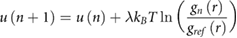
where u(n) is the pairwise interaction potential at iteration number n, kB the Boltzmann factor, T the temperature, gn(r) is the radial distribution function for the nth iteration, gref(r) is the target distribution function obtained from the atomistic simulation and λ is the relaxation parameter controlling IBI convergence. The initial guess for each potential was based on Boltzmann inversion of gref(r). λ stabilizes the scheme and takes values of 0.1 (n ≤ 5), 0.25 (5 < n ≤ 20) and 1.0 (n > 20), respectively. Without λ, water near the graphene/GO froze in the first few iterations, due to a poor initial guess of the potential, leading to convergence problems. For each potential, IBI convergence was assessed using the penalty function, f (n) [63], where
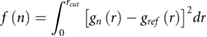
where rcut is the potential cutoff.
Prior to IBI, CG systems with an initial box size of 5 nm and 954 Martini water particles were first pre-equilibrated in an NPT simulation to achieve an appropriate density. For each iteration a 100 ps NVT simulation was performed, followed by 10 ns production run. The initial coordinates of the n + 1th iteration were obtained from the final configuration of the nth iteration and two smoothing steps were applied to the update potential. Various rcut values were investigated.
3.5. Graphene/GO aggregation free energy, ΔF
ΔF was determined from a potential of mean force [64], w(d), using an umbrella sampling approach [65, 66]. The reaction coordinate, d, is the distance between the center of mass of two of the reference sheets shown in figure 1. In the initial configuration, two sheets were arranged parallel in the z-direction in a cubic simulation cell with a side length of 7 nm. The initial distance between the sheets, dmin, was set to 0.35 nm and 0.45 nm for the graphene and GO reference systems, respectively. The initial configurations were then solvated with ~11 000 TIP3P waters or ~2300 Martini water beads, for the atomistic and CG representations. A harmonic potential with a force constant, kd, of 5 × 10⁴ kJ mol−1 nm−2 was then used to pull the GO flakes apart at a rate of 1 nm ns−1 until d = 3.0 nm (dmax). Since the umbrella potential applies only to the center of mass of the two sheets they are able to deviate from their initial parallel arrangement and rotate freely in all three dimensions of the simulation cell. This contrasts with many simulation studies in the literature which enforce an aggregation pathway in which the two sheets are perfectly parallel to each other and aggregate only in the out-of-plane direction. The trajectory from this simulation was used to obtain initial coordinates for individual umbrella sampling simulation windows, which were spaced at d intervals of 0.05 nm in the range from dmin to dmax. In each simulation window, the system was first equilibrated for 100 ps in the NPT ensemble, followed by an NVT equilibration simulation and an NVT production simulation. In the atomistic system the NVT equilibration and production simulations were 2 ns and 4 ns long, respectively. In the CG system, the NVT equilibration and production simulations were 1 ns and 100 ns long, respectively. The reason for the difference in simulation length is that the CG system was faster to equilibrate but was accompanied by a larger integration error, thus a longer production run is required to obtain ΔF to within a similar degree of uncertainty. For both atomistic and CG systems, d was restrained by force constants of 1 × 10⁵ kJ mol−1 nm−2 and 1 × 10⁴ kJ mol−1 nm−2 in the NPT and NVT simulations, respectively. The final ΔF was obtained as the difference in w(d) between the aggregated (the minimum value of w(d)) and exfoliated (dmax) states and its uncertainty estimated using block averaging. w(d) was calculated by unbiasing and recombining the set of biased probability distributions from the umbrella sampling windows using the weighted histogram analysis method [67, 68]. For each system, the reverse process (starting at dmax) was also calculated to ensure reversibility and validity of the method employed to calculate ΔF.
ΔF was computed for the two reference systems shown in figure 1 as well as two additional systems. The first additional system was a deprotonated version of the GO reference system shown in figure 1(b). The second was the deprotonated GO reference system with four additional type C particles. In the atomistic representation of deprotonated GO, a total charge of −1.0e was enforced on the COO− functionality by adjusting the partial charge of the carbon atom after removal of H. In the CG representation of deprotonated GO, a charge of −1.0e was added to type C particles. For the deprotonated simulations, electroneutrality was maintained by the addition of K+ ions. K+ was modelled using the Joung–Cheatham [69] and Martini potentials [39], in the respective atomistic and CG representations.
4. Results and discussion
4.1. Pristine graphene
Radial distribution functions from the atomistic simulation of pristine graphene in water are shown in figure 2. At radial distances greater than ~0.9 nm, g(r) for molecular and clustered waters are identical. However, the position of first maximum shifts to a greater distance upon clustering, associated with loss of resolution at short distances. For gAW(r) there is weak structuring and a peak at 0.56 nm in the clustered case, shifted from 0.40 nm in the molecular case. For gBW(r), a much stronger peak is evident at 0.50 nm, shifted from 0.39 nm in the molecular case. The water surrounding graphene does not become representative of the bulk, giW(r) = 1, until approximately 1.6 nm.

Figure 2. Molecular (dashed lines) and clustered (solid lines) radial distribution functions for (a) gAW(r) (black) and (b) gBW(r) (red), obtained from an atomistic simulation of the reference graphene system in water.
Download figure:
Standard image High-resolution imageThe final CG potentials after 200 IBI iterations and g(r) at selected iterations are shown for A–W and B–W pairs in figures 3(a) and (b), respectively. Using the initial guess of the CG potential (n = 1), g(r) was in poor agreement with clustered atomistic simulations. The potentials drastically improved up to n = 25 and continued to evolve up to n = 100, although the radial distribution functions were relatively insensitive to changes in the potential beyond n = 25. Figure 3(c) shows the penalty function for both CG potentials. No further improvement of agreement with the reference g(r) was achieved beyond n = 100, so the IBI process was finally stopped at n = 200. Fluctuations in f iw(n) for n > 100 were attributed to statistical uncertainty arising from the MD simulations.

Figure 3. IBI for (a) A–W and (b) B–W interactions. In each case the orange line shows the final potential after 200 iterations, uiW(r). The black/red solid lines are the reference g(r) obtained from atomistic simulations and the black/red dashed lines show the radial distribution functions at the iterations denoted by symbols. (c) the penalty function, f iw(n), for each interaction type, with the bold line showing convergence with a line of best fit for n > 100.
Download figure:
Standard image High-resolution imageThe final, converged, CG potential for A–W interactions, uAW(r), has a well depth of −4.6 kJ mol−1 at 0.58 nm. Despite the chemical similarity between A and B type particles, uBW(r) is quantitatively and qualitatively different from uAW(r), with a well depth of just −0.3 kJ mol−1 at 0.59 nm and an energy barrier of 1.2 kJ mol−1 at 0.9 nm. This is thought to be a consequence of the relative length-scales of bonded and non-bonded interactions in the system. Distances between bonded particles within the graphene sheet are much smaller (~0.28 nm) than the typical distances of the nearest-neighbours (~0.5 nm) between graphene and water (see the Martini model [39], in which equilibrium bond distances are typically 0.47 nm), leading to the strong interdependence of uAW(r) and uBW(r) potentials. For instance, this means that water particles adjacent to type B particles at the edge of the sheet also have a relatively strong interaction with type A particles away from the sheet edge. The repulsive barrier in uBW(r) at 0.9 nm prevents the accumulation of too many water molecules at the sheet edges.
For A–W interactions, g(r) was also calculated with a LJ 12-6 potential using parameters in the literature (figure S1 (stacks.iop.org/TDM/7/025025/mmedia)). Firstly, using the parameters of Titov et al [35], a series of intense peaks in gAW(r) were observed, indicating strong layering at the interface. This layering was not observed using our IBI-derived potentials, despite them having a deeper energy well. Secondly, using the parameters of Sergi et al [40], water is repelled from the interface and gAW(r) = 0.05 at r = 0.56 nm (the position where the peak should appear), compared to gAW(r) = 0.87 using the IBI-derived potential. Finally, gAW(r) was also calculated using a LJ 12-6 potential with parameters fitted to the position and energy of the minimum in the IBI-derived potential. Once again, this potential results in a poor prediction of gAW(r). This demonstrates the unsuitability of a LJ 12-6 potential for describing graphene–water interactions at the CG level. This is due to the shape of the potential, which is much too repulsive in the short range region that predominantly determines the first peak in g(r).70
Potentials of mean force for graphene aggregation, w(d), are shown in figure 4, with w(d) shifted to zero at large distances to enable ΔF to be directly extracted from the minimum along the profile of w(d). In the atomistic case, ΔF = −312 kJ mol−1, with the position of the minimum, d0, at 0.36 nm, close to the interlayer distance of bulk graphite. The energy increases rapidly and smoothly for increasing d, reaching a plateau by ~2.0 nm. The deep minimum at short distances and the absence of any energy barrier in the pathway from the aggregated state suggests that water is not capable of producing stable graphene dispersions in the absence of surfactants. Analysis of graphene–graphene configurations at various distances reveals that aggregation occurs via a 'sliding' process, consistent with the results of Lv and Wu [71]. Decomposition of ΔF (table 2) shows that aggregation is favorable both in terms of internal energy (ΔU = −196 kJ mol−1) and entropy (TΔS = ΔU − ΔF = +116 kJ mol−1), thus revealing the important role played by entropy in driving the aggregation of graphene in water. ΔF for the reverse pathway was −311 kJ mol−1, with exact overlap of w(d) demonstrating the reversibility and validity of the employed method. Analysis of interaction energies shows that aggregation is primarily driven by a combination of strong VDW attraction between graphene sheets (−462 kJ mol−1) and a decrease in the water–water energy (−96 kJ mol−1), which is only partly compensated by a decrease in graphene–water energy (+368 kJ mol−1). The average graphene–graphene interaction energy in the aggregated state corresponds to 4.1 kJ mol−1 atom−1, within the range reported in experiments and other simulations.72
Table 2. Summary of thermodynamics of atomistic (AA) and CG graphene/GO sheet aggregation, including decomposition into internal energy and entropy components, and sheet–sheet equilibrium distances, obtained from potential of mean force calculations. The numbers in brackets denote statistical uncertainties.
| model | d0 (nm) | ΔF (kJ mol−1) | ΔU (kJ mol−1) | TΔS (kJ mol−1) | |
|---|---|---|---|---|---|
| graphene | AA | 0.36 | −312(1) | −196(14) | +116(15) |
| CG | 0.34 | −316(3) | −666(2) | −350(5) | |
| GO (pH < 4) | AA | 0.51 | −108(3) | −329(13) | −222(16) |
| CG | 0.45 | −109(4) | −241(2) | −131(6) | |
| GO (pH > 4) | AA | 0.48 | −96(3) | −462(14) | −366(17) |
| CG | 0.44 | −98(3) | −192(2) | −94(5) | |
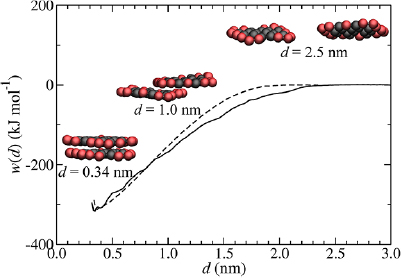
Figure 4. Atomistic (dashed line) and CG (solid line) potentials of mean force for the aggregation of pristine graphene, with graphene–graphene configurations from the CG representation shown at d = 0.34 nm, 1.0 nm and 2.5 nm.
Download figure:
Standard image High-resolution imageArea-normalized graphene aggregation free energies in the simulation literature range from −140 kJ mol−1 nm−2 to −250 kJ mol−1 nm−2 [71, 73–77]. The wide range can be attributed to differences in graphene sheet size, the graphene–water potential, sheet flexibility and the degree of restraint placed on the mutual orientation of graphene sheets. Normalizing with respect to surface area, the value of −116 kJ mol−1 nm−2 obtained in this work is lower than the range reported in the literature. This can be attributed to a combination of sheet flexibility and size. Cao et al [77] showed that the entropy component associated with lattice vibrations of graphene is not negligible and favors the exfoliated state. Inclusion of sheet flexibility therefore provides entropic stabilization of the exfoliated state, lowering the magnitude of ΔF relative to a model in which sheet flexibility is not considered. Additionally, the small reference sheets employed in this work lead to the increased relative contribution of edge regions, which have a lower average graphene–graphene interaction energy. The normalized free energies of the models developed in this work are expected to scale with sheet size due to decreasing relative contributions of edge regions to ΔF.
During the IBI process for pristine graphene, it was found that the final CG potentials were sensitive to the potential cutoff employed. Ultimately, the choice of cutoff is a trade-off between robustness of the potential (i.e. long enough to get reasonable representation of forces well beyond the potential minimum) and computational efficiency [70]. Using the same cutoff as other short-range interactions in the system (rcut = 1.2 nm), uAW(r) had a repulsive region, peaking at an energy of +0.4 kJ mol−1 at r = 0.98 nm. This potential energy barrier was found to destabilize the aggregated state because its distance from the first graphene sheet was commensurate with the position of the water layer at the opposite interface of the second graphene sheet. This ultimately results from a smaller graphene–graphene equilibrium distance compared to relatively large graphene–water distances, and is a consequence of the '2D' mapping. It has previously been suggested that the transition to a purely attractive tail is dependent on the short-range cutoff employed [78]. It was found that the repulsive region could be eliminated during IBI by increasing rcut. Figure S2 shows the converged potentials, after 200 iterations, using various cutoffs in the range rcut = 1.2 nm to 1.6 nm. Within this range of cutoffs, all potentials were able to reproduce the target distribution functions and they converge with respect to rcut, with almost no difference between potentials obtained using rcut = 1.5 nm and rcut = 1.6 nm. It is important to again note the strong interdependence between the graphene–water potentials shown in figure S2, e.g. use of a 1.2 nm cutoff leads to a deeper energy well in uBW(r) than a 1.6 nm cutoff, which is compensated by the shallower energy well of uAW(r), demonstrating how two combinations of potentials can reproduce the correct target distribution functions. Using rcut = 1.6 nm, uAW(r) has a purely attractive tail. This cutoff distance is thought to be a more appropriate due to the slow decay of gAW(r) to unity, finally becoming representative of bulk water at ~1.6 nm. The results presented herein therefore employ rcut = 1.6 nm for graphene/GO–water CG potentials. All other CG potentials in this work use rcut = 1.2 nm to retain compatibility with the Martini model and prevent a deterioration in computational efficiency. Due to the cutoff sensitivity and the sequential approach to parameterization, we encourage consistency in the use of the models by using exactly the same combination of potentials and cutoffs reported in this paper for future studies.
For the CG potentials of mean force, a LJ 12-6 potential was used to model interactions between sheets of graphene or GO. Initial guesses of the graphene parameters (type A and B) were derived from the atomistic potentials. Specifically, the interaction distance, σA/B, was set equal to that of aromatic carbon atoms in the atomistic model (σA/B = 0.355 nm). This choice was justified by consideration that inter sheet interactions are predominantly perpendicular to the plane and that mapping from atomistic to CG systems is in 2D, i.e. the thickness of a particle in the reference system does not increased relative to the atomistic system. The initial choice of interaction strength, εA/B, was made by summing over the 16 atomistic pairwise interactions that had been incorporated into a single CG particle (εA/B = 4.868 kJ mol−1). However, using these initial parameters ΔF was underpredicted relative to the atomistic model, in spite of both the excellent agreement of graphene–graphene and graphene–water potential energy differences. This discrepancy can be explained by comparison of internal energy and entropy contributions to exfoliation; see table 2. In contrast to the atomistic simulations, where aggregation is favorable both in terms of energy and entropy, aggregation of the CG model is strongly entropically hindered (TΔS = −350 kJ mol−1). It should be noted that coarse graining inherently reduces the entropy of the CG system compared to that of the atomistic system since the entropic contributions from translational, rotational and vibrational modes associated with integrated-out degrees of freedom with the CG particles, are no longer resolved. This leads to a shifted energy-entropy balance [30, 79]. Hence, to compensate for the incorrect CG entropy change, the graphene–graphene interaction strength, εA/B, was increased. The final, optimized value of εA/B is 5.8 kJ mol−1, giving excellent agreement with the atomistic simulations, with respect to the shape of w(d), d0 (0.34 nm) and ΔF (−316 kJ mol−1), as shown in figure 4. The optimized parameters for the LJ 12-6 potential are provided in table 3.
Table 3. Summary of non-bonded CG parameters used in this work. Apart from interactions between graphene/GO and water, which used an IBI-derived potential with no fixed functional form, all other pairwise interactions are modelled using a LJ 12-6 potential. For graphene–graphene or GO–GO interactions, parameters were developed by fitting to atomistic potentials of mean force/ΔF. Cross-terms were obtained using Lorentz–Berthelot combining rules, apart from interactions not involving graphene/GO, which use standard Martini interaction parameters* (i.e. σij = 0.47 nm and εij = 4.0 kJ mol−1 (i = W, j = W), 5.0 kJ mol−1 (i = K, j = K) or 5.6 kJ mol−1 (i = K, j = W). For type C particles, the numbers in brackets are for COO− functionalities.
| i | Mi (g mol−1) | εii (kJ mol−1) | σii (nm) | qi (e) |
|---|---|---|---|---|
| A | 48.043 | 5.8 | 0.355 | 0.0 |
| B | 50.059 | 5.8 | 0.355 | 0.0 |
| C | 45.017 (44.009) | 1.3 | 0.598 | 0.0 (−1.0) |
| D | 82.057 | 1.3 | 0.598 | 0.0 |
| K | 72.000 | * | 0.470 | 1.0 |
| W | 24.000 | * | 0.470 | 0.0 |
| WP/WM | 24.000 | — | — | ±0.46 |
4.2. Graphene oxide
Radial distribution functions from the atomistic simulations of GO in water are shown in figure 5. Similar to the pristine graphene case, clustering leads to a loss of resolution at short distance and a shift of the first peak to a larger distance. For gCW(r), which represents ordering of water around COOH functionalities at the edge of the flake, there is an intense peak at 0.37 nm in the molecular case which broadens, decreases in intensity and shifts to 0.50 nm when water is clustered. There is also a distinct minimum at 0.69 nm. For gDW(r), which represents ordering of water around OH-functionalized regions, the first peak, at 0.40 nm in the molecular case, broadens and shifts to 0.58 nm when water is clustered. The first peak in the clustered gDW(r) is at a greater distance than for other particle types because type D particles have a larger effective diameter due to inclusion of atoms not lying in the graphene plane.
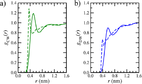
Figure 5. Molecular (dashed line) and clustered (solid lines) radial distribution functions for (a) gCW(r) (green) and (b) gDW(r) (blue), obtained from an atomistic simulation of the reference GO system in water.
Download figure:
Standard image High-resolution imageThe final CG potentials after 200 IBI iterations and g(r) at selected iterations are shown for C–W and D–W pairs in figures 6(a) and (b), respectively. In these simulations A–W and B–W potentials are kept constant and not subject to parameterization (i.e. the same as for pristine graphene as shown in figure 3). An initial guess of the CG potentials (n = 1) provides much better estimates of g(r) compared to the case of pristine graphene (type A and B) particles. As a result, far fewer iterations were required to reach agreement with gref(r) with no further improvement beyond ~40 iterations (figure 6(c)), where f iw(n) = 10−4. The final C–W potential is attractive over the entire range and has a minimum energy of −3.3 kJ mol−1 at 0.5 nm with a weak secondary minimum of −1.1 kJ mol−1 at 1.1 nm. The secondary minimum is necessary to reproduce the secondary peak in g(r), indicating strong water layering around COOH functionalities. However, the D–W potential is repulsive for r < 1.1 nm but has energy minima of 0.4 kJ mol−1 and −0.4 kJ mol−1 at 0.6 nm and 1.2 nm, respectively, separated by a barrier of 1.5 kJ mol−1 at 0.9 nm. The reason for the repulsive potential is that the particle involved (type D) has a larger effective size than adjacent particle types because it includes atoms (OH functionalities) out of the plane of the graphene sheet.

Figure 6. IBI for (a) C–W and (b) D–W interactions. In each case the orange line shows the final potential after 200 iterations, uiW(r). The green/blue solid lines are the reference g(r) obtained from atomistic simulations and the green/blue dashed lines show the radial distribution functions at the iterations denoted by symbols. (c) The penalty function, f iw(n), for each interaction type, with the bold line showing convergence with a line of best fit for n > 100.
Download figure:
Standard image High-resolution imagePotentials of mean force for GO aggregation, w(d), are shown in figure 7. In the atomistic case, d0 = 0.51 nm, which is shifted by 0.15 nm relative to the pristine sheet. The OH functionalities act as spacers, preventing the sheet from residing at a distance that maximizes attractive VDW interactions in pristine graphene regions. d0 is slightly smaller than the experimentally reported average interlayer distance of GO membranes but this could be attributed to variations in oxygen content, imperfect flake stacking and the presence of trapped water molecules in the membrane's interlayer space [80, 81]. For GO, ΔF = −108 kJ mol−1, ~200 kJ mol−1 less favorable than pristine graphene, indicating that the addition of OH functionalities has the effect of stabilizing the exfoliated state relative to the aggregated state. Free energy decomposition shows that, in terms of internal energy differences, GO aggregation is actually much more favorable than pristine graphene aggregation (ΔU = −329 kJ mol−1). However, in contrast to pristine graphene, the aggregated state is strongly entropically unfavorable (TΔS = −222 kJ mol−1), leading to a much reduced ΔF. This suggests that entropy contributes significantly to the stability of aqueous dispersions of GO relative to pristine graphene. Analysis of GO–GO configurations along the profile of w(d) demonstrates that GO aggregation occurs via a similar 'sliding' mechanism as observed for pristine graphene and no water was observed in between the sheets along the entire profile. However, the profile is much less smooth than the pristine graphene case, due to increased surface roughness associated with the OH functionalities, which require realignment of sheets along the aggregation pathway. The largest energy barrier associated with this is 7 kJ mol−1, at d = 1.2 nm.
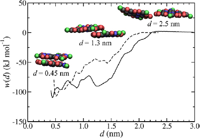
Figure 7. Atomistic (dashed line) and CG (solid line) potentials of mean force for the aggregation of protonated GO, with CG GO–GO configurations shown at d = 0.45 nm, 1.3 nm and 2.5 nm.
Download figure:
Standard image High-resolution imageCompared to pristine graphene the number of molecular simulations studies of the aggregation/exfoliation of GO in aqueous solution in the literature is surprisingly limited, with especially few examples of free energy calculations [75, 82]. In one example, Shih et al [82] calculated the potential of mean force for GO aggregation using fixed parallel sheets and observed minima of 11.6 kJ mol−1 nm−2 and 5.4 kJ mol−1 nm−2 at 0.75 nm and 1.15 nm. Raghav et al also observed significant energy barriers to aggregation [75]. These energy barriers are due to the confinement of discrete water layers in 'stacked' GO–water–GO structures, leading to large oscillations in the solvent mediated forces [12, 76]. Although ΔF is not dependent on the pathway linking the aggregated state to the exfoliated state, modelling the aggregation pathway of two GO sheets in parallel alignment leads to an unrealistic pathway to aggregation with artificially large free energy barriers. Normalizing for surface area, the largest free energy barrier for GO in this work corresponds to ~2 kJ mol−1 nm−2, which is much smaller. This is because our simulations do not place any constraints on the relative orientation of GO sheets. This means they can deviate from the stacked configuration and adopt configurations that lower the energy along w(d). Comparisons with literature suffers from similar problems to pristine graphene (e.g. variations in sheet size, potential model, treatment of flexibility). In addition, the structure of GO is ambiguous, so the specific types and distribution of oxygen functionalities used in the models may also affect results.
For the CG potentials of mean force, additional parameters are required for interactions between sheets involving type C and D particles. As in the case of pristine graphene, atomistic interaction parameters were used to obtain an initial guess of the CG interaction parameters for the LJ 12-6 potential, before fitting εA/B to obtain agreement with the atomistic ΔF. The final interaction parameters for type C and D particles are provided in table 3. For the CG system, ΔF = −109 kJ mol−1, in agreement with the atomistic value, but d0 = 0.45 nm, which is a slightly smaller equilibrium distance than the atomistic simulations. Although ΔF agrees with atomistic case, there are some differences in the shape of w(d); for instance, the CG w(d) decreases much more rapidly from d = 2.0 nm such that at d = 1.2 nm, w(d) = −88 kJ mol−1 in the CG system, compared to −45 kJ mol−1 in the atomistic system. This difference is due to the longer range of CG potentials. Such an acute difference in w(d) at intermediate d was not observed in the pristine case due to σA/B taking the same value in both atomistic and CG simulations. As was the case in the atomistic system, aggregation is energetically favored (ΔU = −241 kJ mol−1) but entropically hindered (TΔS = −131 kJ mol−1), although the entropic component is not as large as in the atomistic system.
Both atomistic and CG simulations predict that the aggregated state of protonated GO is thermodynamically favored over the exfoliated state, suggesting that aqueous GO dispersions are not stable at low pH (<4), in agreement with experiments [15, 83–85]. To understand the origins of the stability of GO dispersions at higher pH (>4), w(d) was also calculated for atomistic and CG systems with all COOH groups deprotonated. When charges were added to type C particles, the IBI-derived potential for C–W interactions, uCW(r), had to be extrapolated at very short distances (r < 0.315 nm) using a quadratic function to prevent instabilities in the simulation (figure S3). These arose because of the weakly repulsive nature of uCW(r) at small r which leads to unphysically close contacts between the GO sheet and polarizable Martini water particles due to electrostatic attraction. Modification of uCW(r) did not affect the simulated results, with identical gCW(r) obtained for protonated GO before and after potential extrapolation. The ΔF resulting from the atomistic and CG w(d) calculations were −96 kJ mol−1 and −98 kJ mol−1, respectively, corresponding to destabilizations of the aggregated state relative to the protonated GO by 12 kJ mol−1 and 11 kJ mol−1. Agreement between these two calculations shows that the CG system reproduces the atomistic system for deprotonated GO well, without the need for further model parameterization. The small decrease in ΔF relative to the protonated GO is due to electrostatic repulsion between GO sheets, which carry a net negative charge. The overall shape of w(d) is similar to the protonated GO system, but less attractive at short distances (d < 1.0 nm).
4.3. Tunable self-assembly of GO
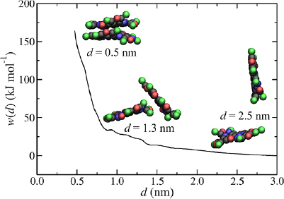
Experiments suggest the stability of GO dispersions is due to electrostatic repulsion of COO− groups [15]. In contrast, ΔF calculated from w(d) for the reference GO system (figure 8) predicts that the aggregated state is thermodynamically stable, with only a small decrease in the aggregation free energy compared to the protonated system. To demonstrate the usefulness of the new CG model and help understand the origin of this apparent contradiction, w(d) was recalculated for a deprotonated GO system with four additional type C groups at the edges of the reference flake, resulting in a total of 8 C particles. GO has a typical carboxylic acid content of ~10 wt% when oxidized using the Hummers method [86], in agreement with our original (4 C) reference system. However, higher carboxylic acid contents (up to 17 wt%) can be achieved, via multiple oxidation steps [86], close to the carboxylic acid content of the 8 C model (19 wt%).

Figure 8. Atomistic (dashed line) and CG (solid line) potentials of mean force for the aggregation of deprotonated GO, with CG GO–GO configurations shown at d = 0.44 nm, 1.3 nm and 2.5 nm.
Download figure:
Standard image High-resolution imageAddition of four more C particles leads to a significant change in the shape of w(d) and now the aggregated state is thermodynamically unfavorable (figure 9). Although extraction of ΔF is not possible in this case because there is no energy minimum at short distances, w(d) = +167 kJ mol−1 at d = 0.5 nm. The instability of the aggregated state of the 8 C particle system compared to the reference system arises from a significant increase in electrostatic repulsion. This is both due to the electrostatic energy being proportional to the square of the charge on the particles and inversely proportional to the distance between the charge groups. In the reference system the surface concentration of C groups at the flake edges is low enough that the GO sheets can mutually orient so as to maximize the distance between charge groups. However, in the 8 C system, the surface concentration of C groups is higher so this is not possible. Evidence for this is provided in figure S4, which compares the radial distribution function for C–C interactions obtained from simulation windows centered at d = 0.55 nm for the reference (4 C) and 8 C systems. Intramolecular electrostatic repulsion of nearby type C groups also leads to some out-of-plane deviations of each sheet. The results suggest that GO sheets should spontaneously exfoliate in aqueous solution, in agreement with experiments performed at pH > 4 [15, 83–85], providing that the edge concentration of COO− functionalities is sufficiently high. As well as increasing the concentration of COO− groups, stabilization of the dispersed state could be achieved by increasing the sheet size, hence increasing the number of charged groups.
Figure 9. CG potential of mean force for aggregation of a deprotonated GO sheet with four additional C groups, with GO–GO configurations shown at d = 0.5 nm, 1.3 nm and 2.5 nm.
Download figure:
Standard image High-resolution image
5. Conclusions
The CG models developed in this work increase the computational efficiency of simulations of aqueous graphene/GO solutions by a factor of ~20 compared to atomistic models and are able to reproduce sheet–sheet aggregation free energies, which are critical in determining self-assembly processes. The employed tabulated numerical potentials correctly reproduce radial distribution functions at the graphene–water interface, unlike simulations employing a Lennard Jones 12-6 potential. Decomposition of atomistic aggregation free energies also highlights the pivotal role played by entropy in the aggregation of graphene/GO in aqueous solution. For pristine graphene, entropy favors aggregation, but for GO, entropy hinders aggregation, so is partly responsible for the stability of aqueous GO dispersions. Aggregation of graphene/GO was not found to proceed via energy minima associated with intermediate 'stacked' structures with discrete confined layers of water, but rather with one sheet sliding over the top of another. This work also reaffirms the importance of acidic groups on GO; if present at sufficiently high surface concentration, COO− functionalities stabilize the exfoliated state by electrostatic repulsion.
The availability of these new CG models enables simulations of graphene and GO in aqueous environments to be performed, without the length and time-scale limitations inherent to atomistic simulations. Within the modelling framework presented, the effect of sheet size and oxygen content on self-assembly could be investigated, offering new insights into the stability of GO dispersions. The model could be extended to incorporate additional structural features of GO, such as pinhole defects and epoxide functionalized regions, or to model reduced GO. The aqueous solutions could be tuned to predict the necessary range of conditions for stable GO dispersions, for instance by varying the pH, ionic strength and presence of surfactants. The models could also be employed for the high-throughput screening of surfactants or solvents for pristine graphene or to predict the fate and transport of graphene/GO flakes in the aquatic environment. Alternatively, the models could be used to optimize the performance of multilayer GO membranes for nanofiltration, in which water flux is dependent on nature of the pore walls [87]. For instance, the relative importance of commensurate stacking of pristine and oxidized regions of the flakes and the role of surface heterogeneity, which occurs over length scales beyond those accessible to atomistic simulations, is yet to be resolved. Finally, the models could be used for the rational design of graphene/GO–containing macroscopic structures, for instance those used in photovoltaic and other electronic devices [88].
Acknowledgments
The authors thank the Engineering and Physical Sciences Research Council for funding this research (Grant reference: EP/R033366/1). The authors would like to acknowledge the assistance given by Research IT, the use of the Computational Shared Facility and the use of The HPC Pool funded by the Research Lifecycle Programme at The University of Manchester.
Supporting information
Contains figures S1–S4 and topology files for reference systems in Gromacs (.itp) format as well as the final tabulated numerical CG potentials and forces for graphene/GO–water interactions.