

Abstract
Vibrational distributions of electronically excited states of N2 obtained through dipole-allowed radiative transitions provide an important tool to study the kinetics of non-equilibrium plasmas under various discharge conditions. In this work, we report, for the first time, streamer-induced visible/near-infra-red emission spectra developing during the first hundred nanoseconds after the initiation of the discharge. Emission through the first positive system of N2 was acquired in 500–1100 nm range, which allows a complete analysis of the N2(B = 0–21) vibrational manifold. The investigated evolution of the vibrational distribution of the N2(B
 , v = 0–21) state at the centre of the gap corresponds to the transition of the streamer head and the subsequent decay of the streamer channel. We show that the vibrational distribution characterising streamer head is determined by Franck–Condon factors, while during streamer relaxation, it is influenced by the complex interaction between triplet excited states of N2. Additionally, the observed N2(B
 , v = 13–21) vibrational levels are likely produced by the interaction of high vibrational levels of N2(W
 , B'
, B' , B
, B with
with  state. We also provide a detailed kinetic scheme for modelling vibrationally-resolved N2(B
 ) state and compare model results with experimental outcomes.
Export citation and abstract BibTeX RIS

Original content from this work may be used under the terms of the Creative Commons Attribution 4.0 license. Any further distribution of this work must maintain attribution to the author(s) and the title of the work, journal citation and DOI.
1. Introduction
The N2(B ) electronic state plays an important role in mediating collisional energy transfers between electronically excited triplet states of N2. In streamer-based discharges, the vibrational distribution function (VDF) of N2(B
 ) enables tracking streamer-induced kinetics not only in laboratory-scale discharges [1] but also in large-scale streamers belonging to the category of transient luminous events occurring in the upper atmosphere, such as blue jets, halos, elves and red sprites [2, 3]. Moreover, the First Positive System (FPS, N2(B
 )
)  N2(A
N2(A )) is also used to determine the electric field in different nitrogen-containing plasmas [4, 5].
It is well known that the kinetics of the N2(B ) state is very complex because numerous interactions between singlet, triplet and quintet states lead to various elementary processes [6, 7]. During the initiation of the streamer discharge, the N2(B
 ) state is dominantly produced by the electron-impact excitation from the molecular nitrogen ground state N2(X
 ), which implies a Franck–Condon-factor-like (FCF-like) VDF [8]. The vibrational levels of the N2(B
 ) state have energies close to those of the N2(W
 ), N2(B
 ) electronic states and also to the higher vibrational levels of N2(A
 ) metastable state [9]. The state is excited/deexcited radiatively through the FPS with radiative lifetime τ0 = 3–11 µs, Wu–Benesch system (N2(W
 )
)  N2(B
N2(B ), τ0 = 45 µs–1 s) and infrared afterglow (N2(B
 )
)  N2(B
N2(B ), τ0 = 10–45 µs). Moreover, the spontaneous emission and the quenching of the higher excited states N2(C
 ), N2(C
 , N2(D
 and N2(G
 could potentially contribute to its population in the low and high-pressure plasmas, respectively [1].
During the post-discharge, the population of the N2(B ) state by the N2(A
 ) pooling reactions often prevails, which results in a very specific VDF with a preferential population of higher vibrational levels [10]. This is caused directly by the pooling or indirectly, due to the pooling-produced excited
  state radiating to the
  state through the emission called Herman-infrared system (HIR). The
  levels are then collisionally coupled to N2(B
 , v = 10–12) levels [11, 12]. The higher vibrational levels (
 13–15) are dominantly predissociated into atomic nitrogen. However, their observation is possible under rather specific conditions up to v = 22 through the FPS(
 ) bands belonging to the
  = +4,+5,+6 sequences [13–17]. To adequately describe the complex kinetics presented above, it is essential to employ a state-to-state model based on a detailed kinetic scheme with trustworthy rate constants. Thus, the reliable reference experimental data, as provided in this work, play a crucial role in testing and validating such models [18]. These models are not only suitable for predictive numerical simulations but also enable state-of-the-art analysis of experimental data from nitrogen-containing plasmas.
The analysis of UV spectra and Intensified Charge-Coupled Device (ICCD) images performed in part I of this series [19] revealed the dynamics and morphology of the triggered streamer monofilament at a pressure of 200 Torr and allowed us to obtain the reduced electric field,  , evolution in the cathode-directed streamer at the centre of the Dielectric Barrier Discharge (DBD) gap. By analysing the vibrational distribution of the N2(C
 ) state, we demonstrated that Plasma-Induced Emission (PIE) is driven by electron-impact processes within the first nanoseconds, followed by collisional relaxation within tens of nanoseconds, and later by energy pooling processes at t > 80 ns.
This part II focuses on the spectral range between 510 and 1100 nm. We show that during the discharge phase, the most important emission in this spectral window is through the FPS, while moving into the post-discharge phase, the relative intensity of the FPS drops significantly compared to the HIR intensity, which becomes dominant in the afterglow. Using the technique of kinetic series, we collected vis–NIR emission maps covering the streamer channel and streamer afterglow phases. We obtained the corresponding vibrational distributions of the N2(B ) state using advanced analysis of FPS spectra. The experimental VDFs were compared with the outcomes of the kinetic model developed to examine the detailed kinetics of N2(B
 ) state. The paper is divided into following sections: section 2 details the data processing and analysis procedures, leading to the extraction of the VDFs and the description of the developed kinetic model. Section 3 includes a thorough analysis of the measured vis–NIR spectra, determination of VDF of N2(B
 ), comparison with the model, and discussion of the obtained results.
2. Experimental setup and methods
2.1. DBD reactor and ICCD spectroscopy
The experimental setup was described in detail in part I [19] of this work, therefore, we recall only the most important facts. A mono-filamentary streamer discharge is produced in a 4 mm gap in a DBD point-plane electrode geometry, as shown in figure 1(a). A specific high-voltage (HV) waveform based on periodic (10 Hz) bursts composed of two consecutive HV AC waveforms (1 kHz) and a nanosecond HV pulse was used to power the discharge. The HV pulse was superimposed with an appropriate phase shift during the second positive AC half-cycle. Within each burst, the superimposed HV pulse produces a triggered streamer mono-filament that is locked with respect to the pulse onset (typical rising slope is 0.2 kVns−1) and captured in figure 1(b). Untriggered discharges regularly occur during the preceding AC phases (typically one streamer mono-filament per one AC half-cycle), leaving residual electrons that serve as initial charges for subsequent events. All ICCD spectra were acquired from the centre of the gap simultaneously using iHR-320 and Shamrock 303i spectrometers; see figure 1(c).

Figure 1. Simplified sketch of the experimental setup showing the point-plane DBD electrode geometry (a), ICCD image of a fully developed triggered streamer discharge (b) and associated PIE diagnostics (c) [19]. The dash-dot circle in (b) indicates the region of interest (ROI) from which PIE was acquired and analysed.
Download figure:
Standard image High-resolution image2.2. Data processing and analysis
The acquired vis–NIR emission spectra (ICCD kinetic series) were corrected for the spectral response of the respective ICCD spectrometers. Corrected spectra were then analysed using the synthetic FPS emission model [1, 20, 21]. As in the case of the Second Positive System (SPS) and First Negative System (FNS) analysis performed in part I [19], the approach is based on the calculation of a set of band profiles by considering the actual experimental instrumental function of the ICCD spectrometer and assuming a Boltzmann temperature ( = 300 K) to calculate populations of the upper rotovibronic levels of the B
 state. Compared to SPS/FNS, the FPS analysis is much more difficult because the FPS involves more upper vibrational levels, and, as a result, FPS band sequences cover larger spectral intervals with significant overlap between neighbouring sequences. Another problem is related to the fact that the lowest N2(B
 ) vibrational levels produce bands in the NIR range; for example, the FPS(0,0) band emits at 1050 nm [1], while the higher N2(B
 ) levels emit the strongest bands in the visible range (below 650 nm). Figures 2 and 3 show two sets of synthetic FPS band profiles used to analyse the FPS emission acquired with low spectral resolution (using 150 and 300 G mm−1 gratings) and medium spectral resolution (using 1200 G mm−1 grating), respectively. All plotted FPS bands were synthesized for equilibrium rotational temperature
  = 300 K and given instrumental function of the ICCD spectrometer. The relative intensity of the FPS bands corresponds to the same (unit) population of all vibronic levels; therefore, each FPS band contributes to the resulting complete FPS spectrum through a weight given by the respective multiplication factor (given by the VDF). It can also be seen that for the analysis of higher (
 ) vibrational levels, the best choice is the spectral range between 500 and 650 nm, as shown in figures 2(a) and 3, while in the case of the lowest (v < 3) levels, the interval 850–1100 nm is a must, see figure 2(b). This implies the need for (and justifies the use of) two different ICCD spectrometers. Each spectrometer is optimized for a different spectral range, aiming to obtain the FPS(
 ) emission (
 = 0, +1,...,+5 sequences) in the interval 500–1100 nm and subsequently, to complete VDF of the N2(B
 ) state. To determine the tail of the VDF, the spectral interval between 500–580 nm containing many FPS bands originating from high vibrational levels (v > 10) is particularly important. However, this spectral range is affected by interfering bands originating from other emission systems as discussed further in the text. Therefore, a higher spectral resolution, such as demonstrated in figure 3, is needed to correctly distinguish the FPS band structures from other N2 and N
 bands, especially during the first few nanoseconds.
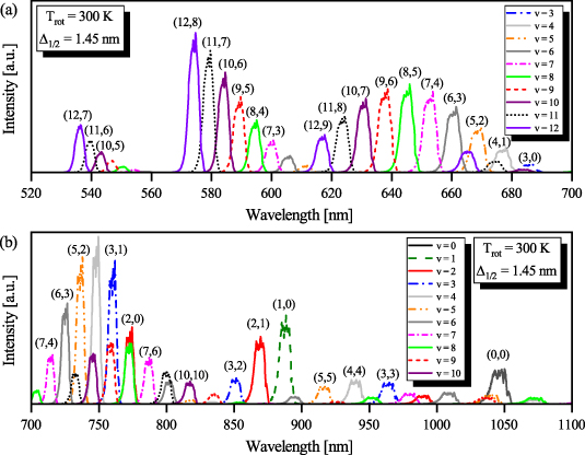
Figure 2. Synthetic FPS bands used to analyse experimental data obtained during the first nanoseconds ( ns). This set of synthetic FPS band-profiles was used to obtain vibrational distribution of the N2(B
 ) state by reproducing time-resolved FPS emission. Individual FPS bands were synthesized for equilibrium rotational temperature
  = 300 K and real instrumental function of the ICCD spectrometer. The parameter
  represents the instrumental function—full width at half maximum of experimentally determined instrumental function at given slit width.
Download figure:
Standard image High-resolution image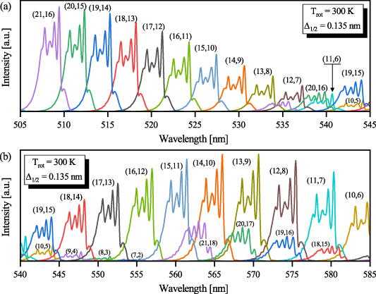
Figure 3. Synthetic FPS bands used to analyse experimental data obtained during the first nanoseconds ( 100 ns). This set of synthetic FPS band-profiles was used to analyse higher vibrational levels (v > 10) of the N2(B
 , state by reproducing time-resolved FPS emission acquired at medium spectral resolution (1200 G mm−1 grating). Individual FPS bands were synthesized for equilibrium rotational temperature
  = 300 K. The parameter
  represents the instrumental function—full width at half maximum of experimentally determined instrumental function at given slit width.
Download figure:
Standard image High-resolution imageWhen obtaining FPS with high spectral resolution (sufficient to partially resolve the structure of individual bands) and a good signal-to-noise ratio, as developed in [20], a simplified approach based on successive subtraction of synthetic FPS bands within a given sequence from the experimental spectra works quite well, and it allows obtaining VDF with good accuracy. Under the current experimental conditions, i.e. low-resolution spectra acquired at high temporal (ns) resolution (often with very low signal-to-noise ratio  ), such a simplified analytical approach would not work (the error associated with determining the initial part of the VDF would propagate and gradually accumulate toward the end of the VDF). Therefore, we developed and used a more sophisticated approach where the set of populations is fitted using a least-squares technique. The expression to fit the experimental spectrum is the following:
where  is a normalization constant;
 ![$p_v = [\mathrm{N_2(B^3} \Pi_\mathrm{g},\textit{v}\mathrm{)]/}$](https://content.cld.iop.org/journals/0963-0252/33/1/015011/revision3/psstad1c09ieqn66.gif)
![$\mathrm{\sum_{\textit{v} = 0}^{\textit{v}_\mathrm{max}}[N_2(B^3} {\Pi_\mathrm{g}}, \mathrm{\textit{v})}]$](https://content.cld.iop.org/journals/0963-0252/33/1/015011/revision3/psstad1c09ieqn67.gif) is the relative population of the vibrational level v;
is the relative population of the vibrational level v;  is the synthetic spectrum of the vibrational level v that contains the summed contributions of the
  = 0, +1,...,+5 sequences, calculated for a unit vibrational population [1, 20]; and
  is the maximum vibrational level containing bands in the fitted region.
  and the various values of pv
are fitted such that the distance between the experimental spectrum (
and the various values of pv
are fitted such that the distance between the experimental spectrum ( ) and the synthetic spectrum (
 ) is minimal. It is important to note that the proper use of this approach requires the exclusion of spectral intervals with potential overlaps with other emissions, such as atomic lines, SPS bands, HIR bands, etc., from the fitting algorithm. These emissions may be hidden under the FPS spectrum and interfere during specific discharge phases. First, the
  is fitted through a simpler approach where the populations pv
are assumed to follow a Boltzmann distribution at a certain temperature Tv
. Then, the results of the preliminary fit are used as initial parameters for the fit where the vibrational populations can have an arbitrary distribution. This procedure allows convergence for all the spectra analysed in this work.
is fitted through a simpler approach where the populations pv
are assumed to follow a Boltzmann distribution at a certain temperature Tv
. Then, the results of the preliminary fit are used as initial parameters for the fit where the vibrational populations can have an arbitrary distribution. This procedure allows convergence for all the spectra analysed in this work.
2.3. Kinetic modeling
The kinetic model used to describe the population and VDFs of N2(B ) levels is based on the reaction scheme listed in [22]. In comparison with the kinetic scheme presented in [22], we added some reactions and species potentially important for the N2(B
 ) state:
- N2(B
 ) state, which levels are energetically close to N2(B) levels,
 - radiative processes connected with the emission of Wu–Benesch system (N2(W) N2(B)) and infrared afterglow (N2(B) N2(B)) [1],
- predissociation of N2(B) levels based on [16].
- We modified some of the quenching reactions, the products of N2(C) quenching by molecular nitrogen are now considered to be transferred to higher levels of N2(W) and N2(B') states, as suggested in [23].


The kinetic model contains 160 species participating in 7312 reactions. The species are listed in table 1, and the reaction scheme is presented in the supplementary material.
Table 1. Species considered in the full kinetic model( ).
).
| Charged species | e, N , N , N
|
| Neutral species | N2(X ,v = 0–58), N2(A ,v = 0–58), N2(A ,v = 0–21), N2(B ,v = 0–21), N2(B ,v = 0–21), ,v = 0–21), |
N2(B ,v = 0–21), N2(W ,v = 0–21), N2(W ,v = 0–21), N2(C ,v = 0–21), N2(C ,v = 0–4), ,v = 0–4), | |
N2(C ,v = 2–3), N(4S), N(2D), N(2P) ,v = 2–3), N(4S), N(2D), N(2P) |
( ) conditions considered: p = 200 Torr,
  = 300 K
The initial value problem for the reaction-resulting ordinary differential equations is integrated in time using an implicit solver, RADAU5 [24], with the reduced electric field  as a parameter. The
  profile was obtained using the FNS/SPS intensity ratio method, as described in part I [19]. The non-zero initial densities
  ,
,  and N(4S) are set according to the experimental results of [25, 26] to be 1013, 1013 and 7 × 1014 cm−3, respectively, since, a certain density of these species is already built up within two breakdowns preceding the third breakdown (during which measurements were performed) [25, 26]. The initial electron density was defined to achieve a maximum electron density between 1013 and 1014 cm−3 and to obtain the best agreement with the experimental data of [25]. In the model at the current conditions, the excited states are produced by electron impact excitation from the
  , and we consider that the specific vibrational level populations correspond to FCF-like distribution. The excited states can be converted to other states in intramolecular and intermolecular energy transfers. During the intramolecular energy transfer, the collisional partner (in this work purely
  ) of the excited electronic state N2(Z) does not change its vibrational level:
and therefore, intramolecular energy transfers can be probable in the case of the low energy difference between the reactant (N2(Z, vʹ)) and the product (N2(Y, vʹʹ)) vibrational levels. The considered intramolecular energy transfers are between the N2(B ) and N2(A
 ), N2(W
 ), N2(B
 ), N2(C
 ) states, because the selection rules in the process allow just u
 g transitions for homonuclear molecules, and we assume that the allowed transitions are favoured in the collisional transitions.
In the intermolecular energy transfer, the energy lost by the quenching of the excited state transfers to the higher vibrational levels of the collisional partner (in this case to  ):
):
The experimental distinction between the intramolecular and intermolecular processes was made just in one rare study [27], where the authors found out that the intramolecular and intermolecular components defining the transfer of N2(A ) and N2(W
 ) states into the N2(B
 ) state are comparable. The theoretical differentiation between the intramolecular and intermolecular processes applying the Landau–Zener and Rosen–Zener approximations was performed by Kirillov [28–30] and similar calculations were also done to obtain the rate constants for intramolecular and intermolecular processes to construct the kinetic scheme for the presented model.
The Rosen–Zener approximation is used for {N2(A ), N2(W
 ), N2(B
 )}
)}  N2(B
N2(B ) endothermic and N2(B
 )
)  {N2(A
{N2(A ), N2(W
 ), N2(B
 )} exothermic transitions [28]. Furthermore, the Rosen–Zener approximation is used for intermolecular transitions defined by the equation (3) for all combinations of
  , where Z,
  N2(A
N2(A ), N2(W
 ), N2(B
 ), N2(C
 )} and also for N2(B
 )
)  N2(B
N2(B ) transition. The Rosen–Zener approximation is defined as:
where  10−10 cm3s−1, γ = 105 cm−1 (
 10−9 cm3s−1, γ = 200 cm−1 for collisions involving N2(C
 )). Note that the k0 and γ used in this work are those recommended by [23, 29, 31] based on comparison with experimental data. The gY
factors are statistical weights denoting the degeneracy of given electronic states,
)). Note that the k0 and γ used in this work are those recommended by [23, 29, 31] based on comparison with experimental data. The gY
factors are statistical weights denoting the degeneracy of given electronic states,  for
for  {N2(B
{N2(B ), N2(W
 ), N2(C
 )} and
  for
for  {N2(A
{N2(A ), N2(B
 )}. The temperature T stands here to express the dependence of the rate coefficient on the neutral gas temperature, and T0 is the room temperature, but in this work, we set
  K. The f represents the Franck–Condon factors used during the transition, where
  and
and  for intramolecular and intermolecular processes, respectively. The used Franck–Condon factors are from [32]. The energy differences were calculated using the following formulas:
  and
and  for intramolecular and intermolecular processes, respectively. The energy levels of the investigated electronic states were calculated using formulas and vibrational constants from [33]. The vibrational levels of N2(B
 ) and N2(A
 ), N2(W
 ), N2(B
 ), N2(C
 ) states considered in the model are shown in figure 4 and labelled with solid lines (higher levels marked by dashed lines were not implemented because of missing FCFs). The Landau–Zener approximation is applied to {N2(A
 ), N2(W
 ), N2(B
 )}
)}  N2(B
N2(B ) exothermic transitions and it is the same for endothermic transitions N2(B
 )
)  {N2(A
{N2(A ), N2(W
 ), N2(B
 )} [28] as:
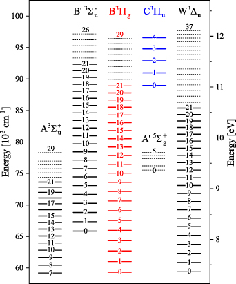
Figure 4. Energy-level diagram for N2(A ), N2(B
 ), N2(B
 ), N2(C
 ),
),  and N2(W
 ) electronic states based on the molecular constants from [33, 34]. The levels with solid lines are included in the kinetic model.
Download figure:
Standard image High-resolution image
where β = 0.466 cm−1K−1. Note that the definition of rate constants as described using equations (4) and (5) also satisfies the principle of detailed balance for reverse rate constants applied for intramolecular processes:
The computation of the processes included in the scheme was performed by the testing the  and
and  values for all
  ,
,  and
and  ,
,  ,
,  combinations for intramolecular and intermolecular processes, respectively. The processes with rate constants higher than 10−13cm3s−1 were then incorporated to the kinetic scheme. The rate constants calculated in the model depend on the
  and k0 parameters, which were set based on the comparison of rate constants with the experimental data of [6, 35], see [29].
Finally, we would like to underline the limits of the developed model. The model does not take into account the rotational structure of the vibrational levels since  and f are computed considering rotational number J = 0. This might influence the results since in general at
  = 300 K the transition does not necessarily occur only between
  and
and  . However, the development of the presented model appears to be the first logical choice for an approach to complex kinetics of the N2(B
 ) state. Moreover, the number of the vibrational levels
  used in the model corresponds with the available Franck–Condon factors in [32]. Up to now, the most detailed N2 kinetic scheme was developed by [30] to study N2(B
 ) state distribution in ionosphere.
3. Results and discussion
All ICCD spectra were acquired simultaneously using iHR-320 and Shamrock 303i spectrometers operating in kinetic series mode using various multi-channel plate (MCP) gates and steps (from a minimum gate of 2 ns to hundreds of nanoseconds). The two ICCD spectrometers acquired the FPS emission between 500 and 1100 nm. Specifically, they collected  = +5, +4, +3, +2, and +1 sequences occurring between 500 and 900 nm in the case of iHR-320 and 620–1100 nm in the case of Shamrock 303i. With the Shamrock 303i spectrometer, we focused mainly on the
  = +2, +1, and 0 sequences emitting between 830 and 1100 nm. After correcting for the relative sensitivity (the wavelength response of the detection chain: collecting optics + spectrometer + ICCD), spectra from different, (but always sufficiently overlapping) spectral intervals were stitched together to obtain a complete spectrum covering the spectral interval. The vast majority of spectrometric data was collected using low-dispersion gratings (150 and 300 G mm−1). However, due to the overlap of the FPS bands with the SPS bands in the spectral region 500–580 nm during the first tens of nanoseconds, it would not be possible to correctly determine the VDF of the N2(B
 ) state for higher vibrational levels (
 ). Therefore, we additionally used a 1200 G mm−1 grating to cover the interval between 510 and 585 nm to get sufficiently resolved spectra, enabling a more accurate evaluation of higher vibrational levels (
 ) not only during the first nanoseconds (possible interference with SPS bands) but also during the afterglow phase (possible interference with Gaydon–Herman green (GHG) bands).
Figure 5 shows an example of time and space-resolved emission spectra obtained with the iHR-320 spectrometer in the interval 500–800 nm. Panel (a) reveals the evolution of the PIE along the DBD gap (spectra registered in multi-track mode integrating the first 5 nanoseconds after the discharge start). Panel (b) then reveals time-resolved spectra obtained from the centre of the gap using a 2 ns MCP gate and the same gate step (single ICCD track registered in kinetic series mode).
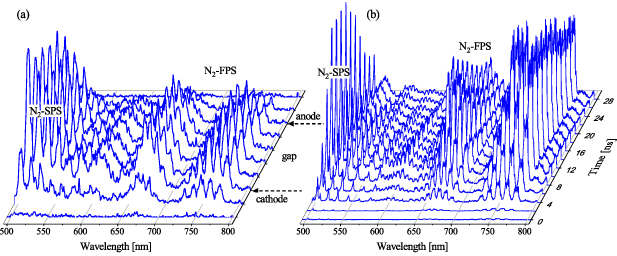
Figure 5. Time and space-resolved vis–NIR emission acquired using iHR320 spectrometer: (a) multi-track mode spectra along the DBD gap acquired using slit of 1000 µm, 150 G mm−1 diffraction grating, integrating over 5 ns interval, and (b) single-track mode spectra acquired in kinetic series (time step of 2 ns and MCP intensifier gate of 2 ns) using input slit of 50 µm and 300 G mm−1 diffraction grating. ICCD spectra were acquired starting from the onset of the triggered discharge, averaging 1000 (a) and 5000 (b) triggered events per one spectrum.
Download figure:
Standard image High-resolution image3.1. Analysis of vis–NIR spectra
One problem to overcome is that other spectral systems can potentially interfere with the FPS emission in the investigated spectral range. This is clearly shown in figure 6(a), which presents three spectra for comparison: one from the beginning of the discharge and two spectra from different post-discharge phases. The upper curve (2 ns MCP gate delayed by 2 ns after discharge onset) shows the FPS spectrum strongly disturbed by SPS emission in the 500–600 nm interval. The overlapping of the SPS and the FPS in this interval provides a valuable link to the SPS emission in the UV region, in particular, the vibrational distribution determined for the N2(C state (cf. figure 10 in [19]) can be used to separate SPS from FPS since this interval is important to determine the N2(B
 ) levels. The middle curve in figure 6(a) illustrates the post-discharge phase (40–60 ns) with significantly reduced SPS emission, in which the entire spectral interval is practically dominated by FPS, with a small exception given by the weak but still observable SPS(0,6). The shape of emission spectra between 510 and 560 nm shows characteristics of the FPS bands originating from high vibrational levels (v > 13). The third, lower curve in figure 6(a) reveals a very different picture when N2(A
 ) metastables come into the game. The PIE starts to be controlled by the N2(A
 )+N2(A
 ) energy pooling; consequently, two other spectral systems emerge and overlap with FPS, namely HIR system (
 with
with  ) and GHG system (N2(H
 )
)  N2(G
N2(G )). Note that the GHG system was observed in high-purity nitrogen [1, 36]. Intense FPS(2,0) band is clearly distinguishable from the FPS due to the high pooling rate for production of N2(B
 ) as suggested in [10]. As a result, the FPS analysis becomes very difficult for longer post-discharge times (hundreds of nanoseconds) unless appropriate subtractions of the dominant HIR and GHG bands are made.
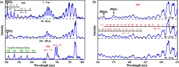
Figure 6. Time-resolved emission spectra obtained in the centre of the gap: (a) comparison of the discharge (2–4 ns) and post-discharge (40–60 ns, 160–200 ns) spectra, and (b) zoom into 550–675 nm region containing FPS bands originating from the highest vibronic levels. All spectra were acquired using iHR320 spectrometer (300 G mm−1 diffraction grating and input slit of 50 µm), accumulating 5000 triggered events per spectrum. All time windows are given relative to the start of the triggered discharge and the respective intensities are not to scale.
Download figure:
Standard image High-resolution imageFigure 6(b) zooms in the 550–675 nm spectral region where the most intense FPS bands originating from the higher vibrational levels are found. For a proper VDF analysis of the B state, it is clear that the overlap of the SPS bands with the FPS (e.g. the SPS(1,9) band overlaps the FPS(12,8) at 575 nm) can be neglected for delays greater than 20 ns (compare the upper spectrum with the middle and the lower spectrum in figure 6(b)).
Figure 7(a) shows ICCD spectra obtained using a Shamrock 303i spectrometer in the 620–1080 nm. The upper curve (integrating the first five nanoseconds after the start of the discharge) shows the FPS spectrum, which is characterized by a relatively weak intensity of the FPS(0,0) band at 1050 nm as compared to FPS bands around and below 750 nm and originating from higher v-levels ( ). After only 20 nanoseconds (see the middle curve in figure 7(a)), there is a clear trend characterized by an increase in the intensity of FPS(0,0) relative to all other bands. This indicates continued relaxation in the N2(B
 ) manifold, which is consistent with the relaxation also observed in the N2(C
 state (cf Part I [19]). Finally, after another 20 nanoseconds, the FPS spectrum is dominated by bands originating from the lowest three N2(B
 ) state levels (
 ).
).
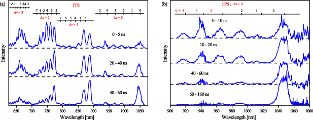
Figure 7. (a) Comparison of the discharge (0–5 ns) and post-discharge (20–40 ns, 40–60 ns) vis–NIR emission. ICCD spectra were acquired using a Shamrock 303i spectrometer (150 G mm−1 diffraction grating and input slit of 150 µm), accumulating 15 000 triggered events per spectrum. (b) Comparison of the discharge (0–10 ns) and post-discharge (10–20 ns, 40–60 ns and 60–160 ns) vis–NIR emission. ICCD spectra were acquired using a Shamrock 303i spectrometer (300 G mm−1 diffraction grating and input slit of 250 µm), accumulating 10 000 triggered events per spectrum. All time windows are given relative to the start of the triggered discharge, and the respective intensities are not to scale.
Download figure:
Standard image High-resolution imageComplementary evidence of the rapid intensity evolution of the FPS(0,0) band relative to all other bands is given in figure 7(b), which shows spectra obtained with better resolution (300 G mm−1 grating). Furthermore, the spectral range 950–1080 nm seems to be particularly suitable for studying the evolution of the  levels, since even after the onset of HIR emission (cf figure 7(b)) due to energy pooling processes, there is no apparent interference of the FPS bands with the HIR bands.
3.2. Populations and vibrational distributions of N2(B)

The FPS spectra acquired by both spectrometers were fitted using a synthetic model for the FPS emission, as described in subsection 2.2. In order to correctly determine the VDF of  , we had to split the analysis into three wavelength ranges:
- (i)610–900 nm to determine relative populations of v = 1–12 by employing 300 and 150 G mm−1 gratings (iHR320 spectrometer). The lower bound of the wavelength interval was chosen to avoid the influence of SPS emission in the initial times (10 ns). For 10 ns, we can shift the lower bound even to 560 nm.
- (ii)830–1080 nm to determine relative populations of the lowest levels v = 0–3 by employing 300 and 150 G mm−1 gratings (Shamrock 303i spectrometer) through intensities of the FPS(0,0), FPS(1,1), FPS(2,2) and FPS(3,3) bands. Note that the sensitivity of the ICCD decreases drastically for wavelengths higher than 1060 nm, as a result FPS(0,0) is the only band originating from v = 0 level available for the current analysis.
- (iii)510–585 nm to determine relative populations of v = 11–21 by employing the 1200 G mm−1 grating and 100 µm entrance slit (iHR320 spectrometer) in the latter times (10 ns).


Figure 8(a) shows a comparison of the experimental spectrum obtained with a 300 G mm−1 grating and 50 µm entrance slit (averaged over a time interval of 20 ns) with two synthetic FPS band profiles simulated at  = 300 K using the actual instrumental function (determined using a Hg–Ar pencil lamp). It is clear that the band profiles generated by the simulation program [1, 20] reproduce very well the partially resolved band-head structure of the FPS(2,0) and FPS(1,0) bands. We have analysed the FPS(2,0) and FPS(1,0) emission during first 200 nanoseconds. In this time interval we do not see any significant modification of the shape of FPS(2,0) and FPS(1,0) partially-resolved bandprofiles. This means that the rotational temperature of the
  levels does not change significantly and
  = 300 K is a good approximation for using synthetic FPS bands for vibrational analysis in the entire time interval considered in this work.
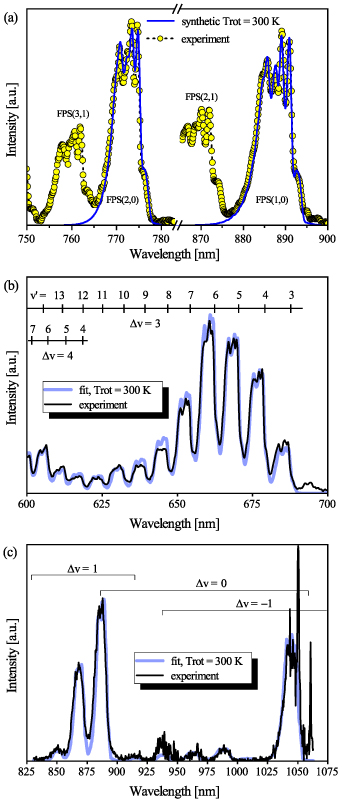
Figure 8. (a) Comparison of experimental and synthetic spectra for  = 300 K, for FPS(1,0) and FPS(2,0). (b) The fit of the experimentally determined FPS spectra obtained by the iHR320 spectrometer at wavelength range 600–700 nm, acquired during 2–4 ns. (c) The fit of the experimentally determined FPS spectra obtained by the Shamrock 303i spectrometer at wavelength 825–1075 nm, acquired during 10–15 ns.
Download figure:
Standard image High-resolution imageFigures 8(b) and (c) shows examples of the fitted experimental FPS spectra, acquired during the 2–4 ns and 10–15 ns by iHR320 and Shamrock 303i spectrometers, respectively. The agreement between the experiment and the fit is overall very good. Note that this interval includes an overlap of the FPS( ,
,  ) bands belonging to the
  = +3 sequence and FPS(
 ,
,  ) bands belonging to the
  = +4 sequence. For example, the level
  contributes to the detected emission close to 610 nm through the FPS(13,10) band and overlaps with the FPS(5,1) whose radiative probability is roughly one half of FPS(13,10); however population ratio between
  and
and  is about 20–25. Therefore, FPS(13,10) band intensity is much lower compared with FPS(5,1), consequently, FPS(13,10) cannot be simply resolved using 300 G mm−1 grating. To study
  , it is necessary to observe the FPS(13,9) at 570 nm, where there is less significant overlap and higher transition probability (about 6 times higher) compared with FPS(13,10). In addition, we used better resolution (1200 G mm−1 grating) to get clearer evidence about the
  populations.
In the region 685–700 nm (see figure 8(b)) several bands overlap, namely FPS(14,13), FPS(18,18) with the HIR(4,2) band and therefore this interval was not used to fit experimental spectra. The visible discrepancy observed in figure 8(c) in 930–950 nm is caused by a low signal-to-noise ratio induced by a local drop in the photocathode efficiency in this wavelength region containing the FPS(4,4) band (which was excluded from the VDF analysis).
Figure 9(a) illustrates the difference between the shape of the FPS spectrum simulated for the complete vibrational distribution ( ) and the shape of the FPS spectrum produced by all FPS(
 , vʹʹ) transitions. This difference is caused by a significant variation between the transition probabilities of the FPS(
 , vʹʹ) and FPS(
 , vʹʹ) bands, which more than compensates for the general trend of a decrease in the population of vibrational levels with increasing vibrational quantum number. It is also worth noting that the FPS(
 ,
,  ) bands belonging to the
  = +2 sequence and the overlapping
  = +3 FPS bands between 610 and 660 nm should be taken into account, so the FPS spectrum is correctly reproduced in this spectral interval.
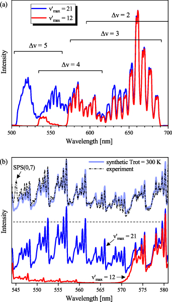
Figure 9. Spectrometric representation of partial ( ) and full (
 = 21) FPS emission: (a) demonstrates the huge difference between full and partial FPS spectrum (simulated for 300 G mm−1 grating, 50 µm entrance slit and
  = 300 K) in the region of Δv = +4 and +5 sequences (i.e. between 500 and 570 nm), (b) compares FPS spectra simulated with experimental results obtained using the 1200 G mm−1 grating, acquired during 30–50 ns.
Download figure:
Standard image High-resolution imageFigure 9(b) compares the synthetic FPS spectrum with the experimental one obtained with much better spectral resolution (1200 G mm−1 grating and 100 µm entrance slit). The blue and red solid curves show the synthetic FPS spectra considering full ( ) and partial (
 ) VDFs, respectively. While the FPS spectrum generated for the partial VDF (red curve) shows a clear separation of the
  = +4 and +5 sequences, the FPS spectrum for the full VDF proves that the region of 500–570 nm is completely dominated by bands (
 ) belonging to the
  = +4 sequence. The agreement is evident when comparing the synthetic FPS spectrum (blue curve) with the experimental data (dash-dot black curve).
The populations and VDFs obtained for v = 1–21 are based on the measurements performed by iHR320 spectrometer, as defined in (i)+(iii). These data are presented in table 2. The VDFs were acquired using MCP gate/step of 2 ns for  ns and the MCP gate/step of 20 ns for t > 30 ns. The error at the initial time 0–2 ns was estimated based on the comparison between various fitting bands belonging to different sequences. The critical for the VDF determination seems to be the incorporation of the 610 - 700 nm region since the bands of the FPS
  sequence are well separated and do not overlap with other bands (except
  ) and, therefore, provide the most trustworthy information concerning a large part of the VDF (
 ). We cannot estimate the error in the fraction of v = 1 since the investigated region includes just FPS(1,0) at 880 nm, but the relative error is probably comparable to the other levels. The VDFs for v = 0–3 were obtained using the Shamrock 303i spectrometer, as defined in (ii) and are listed in table 3. We used the MCP gate/step of 2 and 5 ns for
  ns and the MCP gate/step of 20 ns for t > 10 ns. The appropriate time shift between spectrometers was determined by comparing (i) and (ii) 610 - 900 nm spectra at different times. In both tables 2 and 3, populations are normalized to the
  ; thus, defined as
 ![${[\mathrm{N}_2(\mathrm{B}^3\Pi_\mathrm{g},v)]}/{[\mathrm{N}_2(\mathrm{B}^3\Pi_\mathrm{g},v = 2)]}$](https://content.cld.iop.org/journals/0963-0252/33/1/015011/revision3/psstad1c09ieqn251.gif) . The relative populations obtained by the Shamrock 303i and iHR320 spectrometers were stitched together with respect to
. The relative populations obtained by the Shamrock 303i and iHR320 spectrometers were stitched together with respect to  in order to relate v = 0 population to the data obtained by the iHR320 spectrometer. An interpolation was performed to impose measurements of (ii) with 2/5 ns gates to the measurements of (i) with 2 ns gates. Figure 10 shows a comparison between experimental and model populations of N2(B
 levels. The experimental intensities obtained from the kinetic series were scaled in such a way that the population at the maximum of the experimental curve corresponds to the model value for the given vibrational level (the maxima of the vibrational levels are reached, except for v = 0, between 10 and 20 ns, where the model and experimental VDFs are in reasonable agreement). This allows a simple comparison of the post-discharge evolution for all plotted levels. Figure 10(a) illustrates the evolution of the level populations up to v = 7, revealing a distinctly different trend for the
  and
and  groups. However, in all cases the experimentally observed evolution in early post-discharge (
 ns) is faster compared to the model predictions. The higher levels (
 ) are shown in figure 10(b). The experimental data indicate that the higher vibrational levels decay at very similar rates, which is quite well reproduced by the model results, except for the v = 7 and v = 11 levels.
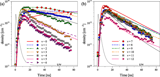
Figure 10. (a) The evolution of N2(B levels from the experiment (points) and from the model (lines). (b) The evolution of N2(B
 levels from the experiment (points) and from the model (lines). The experimental data were scaled in such a way that the maximum of each experimental data for the given vibrational level corresponds to the model value at the time of the maximum. Such scaling was used to compare the decay phase of the experimental data with model results. The black solid curve represents the profile of the reduced electric field used as an input parameter in the kinetic model. The time t = 0 ns corresponds with the maximum of the
  profile.
Download figure:
Standard image High-resolution imageTable 2. Comparison of the experimental and FCF-like VDFs. The experimental VDFs were obtained using the iHR320 spectrometer and averaged over the indicated time interval. The experimental data from 0–2 ns are compared with the FCFs of [32].
| v | FCF-like | 0–2 ns | 2–4 ns | 10–12 ns | 20–22 ns | 30–32 ns | 30–50 ns | 50–70 ns |
|---|---|---|---|---|---|---|---|---|
| 1 |

| 0.52±0.05 |

|

|

|

|

|

|
| 2 |

| 1 |

|

|

|

|

|

|
| 3 |

| 0.95±0.05 |

|

|

|

|

|

|
| 4 |

| 0.80±0.04 |

|

|

|

|

|

|
| 5 |

| 0.53±0.03 |

|

|

|

|

|

|
| 6 |

| 0.36±0.01 |

|

|

|

|

|

|
| 7 |

| 0.22±0.01 |

|

|

|

|

|

|
| 8 |

| 0.12±0.01 |

|

|

|

|

|

|
| 9 |

| 0.044±0.003 |

|

|

|

|

|

|
| 10 |

| 0.033±0.006 |

|

|

|

|

|

|
| 11 |

| 0.022±0.008 |

|

|

|

|

|

|
| 12 |

| 0.010±0.005 |

|

|

|

|

|

|
| 13 |

| — | - |

|

|

|

|

|
| 14 |

| — | - |

|

|

|

|

|
| 15 |

| — | - |

|

|

|

|

|
| 16 |

| — | - |

|

|

|

|

|
| 17 |

| — | - |

|

|

|

|

|
| 18 |

| — | - |

|

|

|

|

|
| 19 |

| — | - |

|

|

|

|

|
| 20 |

| — | - |

|

|

|

|

|
| 21 |

| — | - |

|

|

|

|

|

| — |

|

|

|

|

|

|

|
Table 3. Comparison of the experimental and FCF-like VDFs. The experimental VDFs for N2(B were obtained using the Shamrock spectrometer and averaged over the indicated time interval. All VDFs are related to the v = 2, to stitch these results with the results from iHR320 spectrometer covering v = 1–12.
| v | FCF-like | 0–2 ns | 2–4 ns | 5–10 ns | 10–15 ns | 15–20 ns | 10–30 ns | 30–50 ns | 50–70 ns |
|---|---|---|---|---|---|---|---|---|---|
| 0 | 0.31 | — | 0.42±0.08 | 0.42 | 0.64 | 0.78 | 1.05 | 2.43 | 2.57 |
| 1 | 0.75 | — | 0.60±0.12 | 0.60 | 0.65 | 0.75 | 0.80 | 1.27 | 1.38 |
| 2 | 1.00 | 1.00 | 1.00 | 1.00 | 1.00 | 1.00 | 1.00 | 1.00 | 1.00 |
| 3 | 0.97 | 0.67±0.15 | 0.67±0.15 | 0.67 | 0.52 | 0.44 | 0.36 | 0.27 | 0.26 |
The experimental data show that the population of the higher levels N2(B decay immediately after reaching their peak at approximately 12 ns. The populations of lower levels N2(B
 in the range 12–80 ns grow or do not decay so rapidly as the higher levels. However, this behaviour is not well reproduced in the kinetic model. The most apparent is this behaviour when comparing N2(B
 and N2(B
 . Obviously the N2(B
 should be better populated at the expense of depopulation of N2(B
 . This suggests that pathways (and corresponding rate constants) connecting these states are likely underestimated in the model, or the rate of quenching of individual N2(B
 levels out from triplet states needs to be reevaluated.
The VDFs of  as shown in figure 11(a) present the combination of (i), (ii) and (iii) measurements for times 0–70 ns. During the first interval (0–2 ns), we observe a very good agreement with the theoretical Franck–Condon factors [32]. The agreement is also good for the 10–12 ns time interval, except v > 8. Similarly, as in [19] for the N2(C
 ) state case, the agreement proves the dominant electron-impact excitation from the ground state
  to the excited state N2(B
 ). During the later times (t > 20 ns), the relaxation from higher to lower vibrational levels is evident. At the initial times (0–2 ns, 10–12 ns), the v = 2 has the highest population; however, for the higher times (30–70 ns), the dominance of v = 2 is replaced by the
  vibrational levels. We also observe a local maximum for v = 6 in the VDF. The figure 11(b) shows VDFs of N2(B
 computed using the kinetic model for the same time intervals as in the experiment. The model predicts the local maximum for v = 6 as well as the increase of the VDF for v > 13, which is caused due to the
  and
and  collisional coupling through N2(W
 ) and N2(B'
 ) intermediate states. The local minimum observed in the VDF for
  is due to the coupling of these vibrational levels to the
  levels, which are above the dissociation limit [15, 16]. Geisen et al [16] showed that the predissociation rate constants for
  depend on v and reach the maximum values 3.08×10⁸, 1.71×10⁸, 1.13×10⁸ s−1 for
  , respectively. On the other hand, it is obvious that the presented kinetic model is unable to reproduce the growth of the
  with respect to the v = 2 as observed in the experiment. We observe also a significant difference in the relative populations of
  levels, which is most apparent for t = 10–12 ns. The corresponding VDF fraction
 ![${\sum_{v = 9}^{21}[\mathrm{N}_2(\mathrm{B}^3\Pi_\mathrm{g},v)]}/{\sum_{v = 0}^{21}[\mathrm{N}_2(\mathrm{B}^3\Pi_\mathrm{g},v)]}$](https://content.cld.iop.org/journals/0963-0252/33/1/015011/revision3/psstad1c09ieqn284.gif) is below 0.05 in the experiment while 0.16 in the model. This discrepancy could be due to the missing N2(A
is below 0.05 in the experiment while 0.16 in the model. This discrepancy could be due to the missing N2(A ) and N2(A
 ) states, which are energetically close to the
  levels. The presence of these vibrational levels would lead to the population transfer to the additional states and would decrease the
  populations. More details on the model results will be presented in the following section.

Figure 11. (a) Experimental VDFs of N2(B , normalized to v = 2, for spectra acquired in various time intervals. (b) VDFs of N2(B
 obtained using the kinetic model.
Download figure:
Standard image High-resolution image3.3. Discussion
We were able to obtain the VDFs of the  state in a time interval covering both the formation/propagation phase of the streamer front and the later relaxation phase of the streamer channel. During the initial phase (t < 10 ns), the accuracy of the VDF determination is strongly limited by the low signal intensity (
 ) and the overlap of the FPS bands with the SPS bands (
 ). During the relaxation phase (t > 100 ns), a complete VDF analysis is almost impossible because many FPS bands overlap with the significantly more intense bands of the HIR/GHG systems produced by
  pooling. On the other hand, the fact that the population of both
  and
and  states can be monitored even during the relaxation phase driven by
  metastables [19] offers a unique chance not only to obtain the VDFs of both electronic states but in principle also their absolute densities, as proposed in [37] (out of the scope of present work).
The comparison of experimentally determined N2(B
 evolution with the kinetic model revealed that the pathways connecting N2(B
 with N2(B
 states are probably underestimated in the presented kinetic model. According to the model, existing pathways are not only vibrational relaxations within the N2(B
 state, for example:
but also pathways leading through the intermediate  and
and  states:
and
Note that processes (7)-(11) are those having rate coefficients higher than  . In the literature, the effective rate coefficients for the
  quenching by N2 can be found in many works [9, 10, 38–41]. Some of these works [10, 38, 39, 41] refer that the effective quenching rate coefficient for N2(B
 is at least twice as large as for N2(B
 state, thus, in the agreement with our experimental results. However, the use of the effective quenching rate coefficient is in general misleading since it ignores the structure of the energetically adjacent vibrational levels of different electronic states. The concept based on effective rate coefficients is valid just after creating equilibrium with the energetically closest levels. Therefore, some authors [9] distinguish two quenching rates: fast and slow, where the first corresponds to the population transfer to the energetically closest levels and the second to the quenching after finding equilibrium with the closest levels.
Moreover, the use of the effective rate coefficients in the kinetic models, as it was done, for example, in [18], is not able to predict energy transfers from the higher to lower vibrational levels under highly transient discharge conditions. Therefore, the development of the state-to-state kinetic model, as done within this work, seems to be the only possible way to describe the kinetics of N2(B state correctly.
To the best of our knowledge, no other study determined the complete VDF of  under the streamer discharge conditions. A list of works on
  VDF at different discharge conditions can be found in [42], and in general, we observe similar effects as reported in those works. The VDF observed for t > 20 ns tends to relax towards the lower vibrational levels. We also observe a local VDF maximum for v = 6. This phenomenon is usually connected with the intramolecular coupling of
  and N2(W
 ) states [43] since the
  and N2(W
 ) states have low energy difference, which implies the following process:

with energy difference of 132 cm−1 [32]. The N2(W = 7) state is populated by electron impact with a much higher rate constant than the
  state, therefore during first tens of nanoseconds the N2(W
 = 7) population is converted to energetically close
  state by the process (12). Later, both close states find equilibrium and evolve as a single state.
The FPS radiation observed in the range 510–585 nm, belonging to the ( ) bands, is also quite important for understanding underlying microscopic processes. This radiation is a characteristic of the so-called Lewis-Rayleigh afterglow, which is regularly observed in the flowing afterglow rich in atomic species produced by a continuous discharge in low-pressure nitrogen [44, 45]. In our case of a transient streamer monofilament at high pressure, the origin of radiation from higher (
 ) levels is different. The observed overpopulation of the higher levels
  can be roughly reproduced by introducing the intermolecular coupling of the
  state to the higher levels of N2(W
 ) and N2(B'
 ) states in the kinetic model, as proposed in [23]:
and
The N2(W ) and N2(B
 ) state levels are efficiently coupled to N2(B
 12) and mediate the transfer of
  state population to
  state. According to the developed model [23, 46], the most dominant collisional transfers from
  are to
  and
and  . Similarly,
  and
and  for collisional quenching of
  . Note that, based on results of part I of this work [19], the populations of
  contain approximately 90 % of the total
  state population. The energy of the
  and
and  levels coincides with the energy of N2(B
 ) levels, see figure 4, therefore allowing the intramolecular energy transfers:
which populate the  state during early post-discharge phase.
Since the kinetic model is very complex, it is useful to test the contribution of specific processes on the resulting VDF. Table 4 and figure 12 demonstrate the potential of the selected processes for VDF shaping. The inclusion of the specific processes in the model is denoted using check marks. Insets of figure 12 show the evolution of ![$S = \sum_{v = 13}^{21}[\mathrm{N}_2(\mathrm{B}^3\Pi_\mathrm{g},v)]$](https://content.cld.iop.org/journals/0963-0252/33/1/015011/revision3/psstad1c09ieqn501.gif) in each test case. First four columns allow insight at pressure used in the present experiments (200 Torr). Last two columns with corresponding plots show predictions at pressure of 20 Torr, where the
in each test case. First four columns allow insight at pressure used in the present experiments (200 Torr). Last two columns with corresponding plots show predictions at pressure of 20 Torr, where the  and
and  profiles are set the same as in the case of 200 Torr.
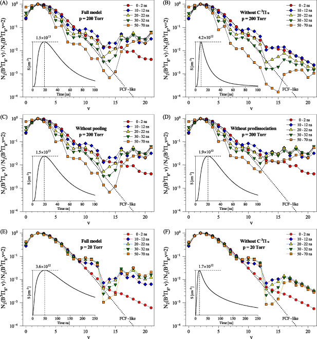
Figure 12. Test of the influence of selected processes on the shape of the VDF of N2(B state. The inclusion of specific processes in the kinetic model for each test case (A)–(F) is specified in table 4.
Download figure:
Standard image High-resolution imageTable 4. Test of the influence of selected processes on the shape of the VDF of N2(B ) state. Each letter in the first row corresponds to a specific test case shown in the corresponding panel of figure 12.
| (A) | (B) | (C) | (D) | (E) | (F) | |
|---|---|---|---|---|---|---|
N2(C ) )  N2(W N2(W )/N2(B' )/N2(B' ) ) | ✓ | — | ✓ | ✓ | ✓ | — |
 pooling pooling | ✓ | ✓ | — | ✓ | ✓ | ✓ |
 predissociation predissociation | ✓ | ✓ | ✓ | — | ✓ | ✓ |
| pressure [Torr] | 200 | 200 | 200 | 200 | 20 | 20 |
The participation of the  to N2(W
 ) and N2(B'
 ) coupling on the
  population is apparent when comparing figures 12(A) and (B). In the test case (B), the population of
  state contributes only by radiative quenching to the population of state
  (low vibrational levels). Obviously, the electron-impact excitation of
  ,
,  and
and  states; which are the levels with energies higher than the energy of
  level brings just 20% of
  population. Therefore, the electron impact excitation is dominant few nanoseconds after the streamer onset, compare the insets of figures 12(A) and (B). Moreover, the electron impact excitation alone is not able to explain the well-defined VDF maximum for
  . There is no difference between figures 12(C) and 12(A), because pooling reactions have just a minor effect on the VDF for t < 70 ns due to low density of
  :
:
However, we cannot definitely exclude the population of  levels from
  and
and  combinations, which are already present tens of nanoseconds after the discharge onset [19].
Figure 12(D) shows that the predissociation of  levels is responsible for the local minimum of the VDF. From the comparison of insets of figures 12(A) and (D), it is apparent that the contribution of the predissociation to the atomic nitrogen production approximately
  cm−3, seems to be just a minor source of the atomic nitrogen [26]. Further insight into the role of collisional quenching of
  on the VDF shape of
  state might be obtained by comparing distributions formed at high pressures (
 200 Torr) with those produced at lower pressures (20 Torr), see figures 12(E) and (F). The fraction of the
  which participates in the collisional quenching can be determined as
 ![${k_\mathrm{q} [\mathrm{N}_2]}\cdot{(1/\tau_0 + k_\mathrm{q} [\mathrm{N}_2])^{-1}}$](https://content.cld.iop.org/journals/0963-0252/33/1/015011/revision3/psstad1c09ieqn526.gif) , where
, where  cm3s−1 is the quenching rate constant for
  quenching by N2 and
  ns is the lifetime of spontaneous emission of the
  state. For the
 ![$[\mathrm{N}_2] = 6.4\times10^{18}$](https://content.cld.iop.org/journals/0963-0252/33/1/015011/revision3/psstad1c09ieqn531.gif) cm−3 density corresponding to the pressure of 200 Torr, we find that approximately 70
cm−3 density corresponding to the pressure of 200 Torr, we find that approximately 70 of the
  population is quenched collisionally. At the pressure of 20 Torr it is 20
 . Consequently, higher pressure leads to populations of higher vibrational levels of
  state, contrary to lower pressure which tends to support population of lower levels through the radiative quenching (SPS).
In figure 13 the evolution of ![$\sum_{v = 13}^{21}[\mathrm{N}_2(\mathrm{B}^3\Pi_\mathrm{g},v)]$](https://content.cld.iop.org/journals/0963-0252/33/1/015011/revision3/psstad1c09ieqn536.gif) and
and  determined by the model is compared with the SPS(
 ) and FPS(
 ) intensity profiles, both normed to maximum. The SPS(
 ) profile was obtained in [19], and the FPS(
 ) profile was obtained by integrating the intensity observed in the interval 500–570 nm. We observe that the time delay between the peaks is approximately 10 ns, which corresponds with
  effective lifetime, in the case of N2 at 200 Torr reaching values
  = (8.0
  12) ns,
  = (4.0
  5.6) ns [47]. The right axis of figure 13(a) presents the evolution of the fraction
 ![${\sum_{v = 13}^{21}[\mathrm{N}_2(\mathrm{B}^3\Pi_\mathrm{g},v)]}/{\sum_{v = 0}^{21}[\mathrm{N}_2(\mathrm{B}^3\Pi_\mathrm{g},v)]}$](https://content.cld.iop.org/journals/0963-0252/33/1/015011/revision3/psstad1c09ieqn547.gif) obtained by model and experiment. The maximum of this fraction corresponds to the peak of the FPS(
obtained by model and experiment. The maximum of this fraction corresponds to the peak of the FPS( ) intensity profile, indicating that the main population of the
  occurs during 10–30 ns.
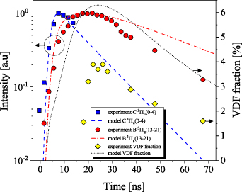
Figure 13. Left axis: comparison of the evolution of FPS( ) and SPS(
 ) intensity profiles. Right axis: evolution of the fraction of the
  and
and  states.
Download figure:
Standard image High-resolution imageWe should discuss also other possible channels to be considered for production of  levels. Such channels could be associated with the atomic species
  and three-body recombination [48]:
where  denotes higher vibrational levels of
  ,
,  and
and  states, which can be converted to
  levels. Nevertheless, the results of the kinetic model show that the densities of
  atoms are rather constant in the time
  ns, therefore the radiation produced in the
  levels should not decay rapidly after reaching the maximum population between 20 and 30 ns.
Further channel could be the following pooling mechanism studied by Piper [49]:
but he did not observe  levels and used a low pressure N2 afterglow at high vibrational temperatures (1800 and 3700 K). We can estimate the magnitude of the source term of (18) in our case:
 ![$P = k\cdot[{\mathrm{N}_2}(\mathrm{A}^3 \Sigma_\mathrm{u}^+)]\cdot[{\mathrm{N}_2}(\mathrm{X}^1 \Sigma_\mathrm{g}^+, v \unicode{x2A7E} 5)]$](https://content.cld.iop.org/journals/0963-0252/33/1/015011/revision3/psstad1c09ieqn565.gif) , the rate constant
, the rate constant  cm3s−1,
 ![$\sum_{v\unicode{x2A7E}0}[{\mathrm{N}_2}(\mathrm{A}^3 \Sigma_\mathrm{u}^+, v)] \approx 10^{15}$](https://content.cld.iop.org/journals/0963-0252/33/1/015011/revision3/psstad1c09ieqn567.gif) cm−3 and the
cm−3 and the ![$\sum_{v\unicode{x2A7E}5}[{\mathrm{N}_2}(\mathrm{X}^1 \Sigma_\mathrm{g}^+, v)] \approx 10^{14}$](https://content.cld.iop.org/journals/0963-0252/33/1/015011/revision3/psstad1c09ieqn568.gif) cm−3 based on the kinetic model. Such values lead to
cm−3 based on the kinetic model. Such values lead to  cm−3s−1, which requires approximately 0.1 ms to build up
  densities 1014cm−3 as predicted by our model. Therefore, this process should not be significant in our case.
4. Conclusions
In this study, which is the second part of the series [19], we investigated the dynamics of the formation of a vibrational manifold of the  state under streamer discharge conditions in pure nitrogen. In the part I, a detailed analysis of the SPS and FNS emissions revealed characteristic VDFs of the
  and
and  states in the middle of the discharge gap starting from the onset of the streamer up to the first microsecond after the streamer head transit.
Here, in part II, advanced in-depth analysis of the vis–NIR emission obtained with nanosecond time resolution provided the state vibrational distribution from the lowest (v = 0) to the highest (v = 21) observable vibrational level. Obtaining such a wide range of vibrational levels of this electronically excited state with nanosecond time resolution is quite unique and was achieved by employing two complementing ICCD spectrometers, which enabled the collection of spectrometric data in the wavelength range from 500 to 1100 nm.
The results of the experiments supported by the results of numerical modeling lead to the following conclusions:
- During the first nanoseconds ( ns) after the discharge onset, the VDF of follows the FCF-like distribution. However, the determination of higher vibrational levels (v > 8) and thus VDF(v > 8) is burdened by a systematic error due to significant overlaps of FPS with SPS bands in the spectral interval between 500 and 600 nm.
- During later times (t > 10 ns) we observe a very different evolution of the lowest vibrational levels () compared to the higher vibrational levels (v > 2), resulting in a significant deviation of the VDF from the initial FCF-like shape. Populations of v > 2 vibrational levels decrease roughly exponentially (early afterglow,
ns) with characteristic decay time constants between 20 and 30 ns. The decrease in the populations of the lowest vibrational levels () appears to be notably slower.
- Thanks to the rapid relaxation of the intensities of the SPS bands, we succeeded to clearly observe the build-up of FPS bands originating from higher () vibrational levels. This build-up peaks between 10th and 20th nanosecond after which FPS band intensities decrease in time. The local VDF minimum driven by predissociation is reached for while the local maximum is reached for levels .
- A state-to-state kinetic model, including the interaction of high vibrational levels of N2(W, B', B with state, explains quite well the main features of the experimentally determined VDFs, such as the overpopulation of the level v = 6 and increase of the tail of the VDF (v > 12). On the other hand, the current model does not reproduce the fine structures of the VDF well, which we attribute to the complexity of the inter- and intra-energy transfer processes that govern the redistribution of the triplet state populations formed by the streamer head electrons. In this context, further extension of the model to higher levels (namely ) and reevaluation of the state-to-state rate constants appear important.


We conclude that experimental data on vibrational distributions of N2 excited states [19, 25, 26, 37] obtained under highly transient discharge conditions (such as a streamer) are of the highest importance for the development/validation of advanced kinetic models [18, 22, 30, 31] and diagnostic approaches [1, 47]. At this point, a better understanding of the build-up and relaxation of all observable electronically excited state VDFs under different pressures and similar (i.e. highly transient)  conditions seems crucial. Corresponding experiments are ongoing.
Acknowledgments
This work was supported by the Czech Science Foundation (Project No. 15-04023S) and by the Strategy AV21 project. V G and T C D were partially supported by the Portuguese FCT-Fundação para a Ciência e a Tecnologia, under funding to IPFN Lab (DOI: 10.54499/LA/P/0061/2020), projects (DOI: 10.54499/UIDB/50010/2020, 10.54499/UIDP/50010/2020 and 10.54499/PTDC/FIS-PLA/1616/2021), and grant PD/BD/150414/2019 (PD-F APPLAuSE). We would like to thank prof. Andrey S Kirillov (Polar Geophysical Institute Murmansk, Russia) for his beneficial advice and the discussion concerning intermolecular and intramolecular energy transfers.
Data availability statement
All data that support the findings of this study are included within the article (and any supplementary files).
Supplementary data (1.3 MB PDF)
Supplementary data (142 kB TXT): complete_kinetic_scheme.txt