

Abstract
We consider systems described by a two-dimensional Dirac equation where the Fermi velocity is inhomogeneous as a consequence of mechanical deformations. We show that the mechanical deformations can lead to deflection and focusing of the wave packets. The analogy with known reflectionless quantum systems is pointed out. Furthermore, with the use of the qualitative spectral analysis, we discuss how inhomogeneous strains can be used to create waveguides for valley polarized transport of partially dispersionless wave packets.
Export citation and abstract BibTeX RIS
1. Introduction
Dirac fermions in graphene cannot be controlled very well by electrostatic fields as they can tunnel through electrostatic barriers [1]. Strain engineering [2] (also called straintronics or origami electronics [3]), attracts increasing attention as a viable option for the design of electronic devices via mechanical deformations [2–10]. Indeed, strains or folds of graphene sheet can be used to create waveguides [2, 10–13]. They can also lead to collimation, focusing or valley polarization of electron beams [2, 10, 14], or to the Kondo effect [15].
In graphene, the mechanical deformation of the crystal is manifested by the appearance of gauge fields [4, 5, 16] in an effective Dirac Hamiltonian and, in this way, it affects the dynamics of Dirac fermions. The mechanical deformation is expressed by a strain tensor u = u(x, y). It is given in terms of the displacement vector u = (u1(x, y), u2(x, y)) and vertical displacement h = h(x, y),

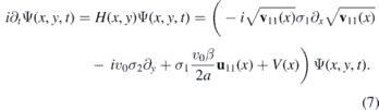
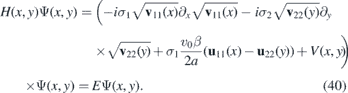
The Hamiltonian of the quasi-particle with the momentum in the vicinity of the Dirac point K then reads6

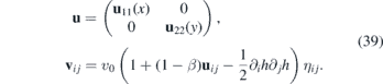
The tensor of Fermi velocity is defined as [17]

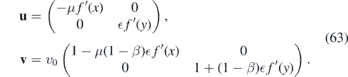
whereas the vector potential and the electrostatic potential V that emerge due to the mechanical deformation are


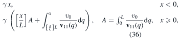
Here η = diag(1, 1), β is the electron Grüneisen parameter and a is the interatomic distance and v0 the Fermi velocity in the strain-free crystal (β ∼ 2–3, a = 1.42 Å and v0 ∼ 106 m s−1 for graphene). The bare value of the coupling constant g has not been fixed definitely yet. In the literature, its value ranges between 0 eV to ∼20 eV, see e.g. [4, 18]. The currently used value is g ∼ 3 eV, see [12]. The linear description of strains (4) and (5) is rather reasonable up to maximum strain 15%–20%, see [19] and references therein. For these values, the electrostatic field would be V ∼ 0.5 eV. In this work, we set ℏ = 1.
The strain in graphene, as well as in other two dimensional materials, can be achieved by putting the material on the substrate that is micro-structured [6] or mechanically deformed [7, 8]. The strain can also appear due to the mismatch of the lattices of the material and the substrate that gives rise to superlattices and associated Moire patterns [9]. It is worth mentioning that there are two-dimensional systems where the Fermi velocity of Dirac fermions is intrinsically inhomogeneous [20, 21]. Let us also mention models for corrugated graphene based on the hybridization of electron orbitals [22] where the effect of the deformation is manifested by an electrostatic potential.
From the theoretical side the impact of strain in connection with the reduction of charge mobility in graphene has been extensively reviewed (see [5] and references therein). The experimental challenges to understand the effect of strain through ripple formation, random strain fluctuations, random gauge field scattering and other mechanisms that compromise the pristine mobility of the material are still an open field. Large variations of the resistance across the samples make it still inconclusive to compare the versatility of graphene in actual nanodevices development as compared with usual semiconductors [23, 24].
The Hamiltonian (2) resembles the energy operator in presence of electromagnetic field. However, it contains the inhomogeneous Fermi velocity that arises due to the shift of the Dirac points caused by the mechanical deformation. The formula (3) for Fermi velocity is obtained when the tight-binding Hamiltonian is linearized around the shifted Dirac point [17, 25] see also [26]. Alternatively, the equation (2) can be obtained by covariant approach based on quantum field theory in curved space–time where the inhomogeneous Fermi velocity is associated with the components of the metric tensor [27, 28]. It is worth mentioning that the latter approach proved to be efficient in the simulation of cosmic strings [16, 29] or black-hole horizons in graphene [30, 31].
In our work, we focus on two specific situations described by the Hamiltonian (2) where the inhomogeneous strain tensor gives rise to the diagonal Fermi velocity with position dependent components. In the next section, we consider the system with diagonal Fermi velocity whose upper component is x-dependent whereas its second non-vanishing component is constant. We analyze the trajectory and deformation of the wave packets that get deflected by inhomogeneous strains. The trajectory can be obtained analytically with the use of a specific transformation that relates the considered system with the free particle model. The scattering of Dirac fermions on the barriers induced by strain in combination with external fields was analyzed e.g. in [10, 32–39] where analogies with optical systems were discussed.
In the third section, we consider the system with diagonal strain tensor whose upper component depends on x, while its lower component is y-dependent. We focus on the analysis of the confinement of Dirac fermions within the waveguide formed by the strain. In literature, there have been already considered explicit models with piecewise constant strains [2, 10, 11], or smooth deformation profiles [12, 13], where the spectrum of models was found numerically, see also [13] for experimental results. We apply another approach based on the qualitative spectral analysis of Dirac equation. It relies neither on the explicit solutions of the stationary equation nor on the explicit form of the strain-induced barrier. We show that the strained system is related to the strain-free model with external magnetic field. Existence of partially dispersionless wave packets in the waveguide is discussed. We use simple criteria [40, 41] to find the strain configurations that lead to appearance of these guided modes. The last section is left for discussion.
2. Deflection of wave packets by mechanical deformations
In this section, we focus on the systems where the mechanical deformation gives rise to the following strain tensor and the associated Fermi velocity,

We are interested in the way the particles propagate through the interface between two regions with asymptotically constant strain. Therefore, we will suppose that u11(x) is a bounded positive function, limx→±∞u11'(x) = 0, such that v11(x) is also bounded and positive with a bounded derivative, limx→±∞v11'(x) = 0. The inhomogeneous strain and Fermi velocity (6) can be induced by a unidirectional strain and/or vertical displacements (3). The corresponding equation of motion for the two-dimensional Dirac fermion is
2.1. The model with step like strain
First, let us briefly review a simple model where the nonvanishing component of the strain tensor and v11(x) are piece-wise constant
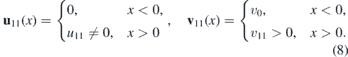
Here we set v0 = 1. The electrostatic potential V(x) is vanishing for x < 0 but it acquires non-zero constant value for x > 0. This model will help to understand the influence of the inhomogeneous Fermi velocity and the electrostatic potential on the scattering of the Dirac fermions, and it will also motivate our further analysis. This setting was discussed in detail in [38] for homogeneous Fermi velocity, see also [36, 37]. For inhomogeneous piece-wise constant Fermi velocity, it was elaborated in [39].
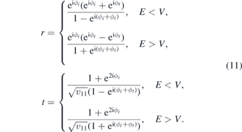
One can find explicit solutions F of the stationary equation separately for x < 0 and x > 0,
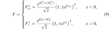
where the indices i, r, t denote incident, reflected and transmitted wave and 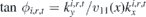 . The index ± corresponds to the sign of the kinetic energy E − V and T denotes here the transposition. The normalization constant comes from integration over a unit volume. We fix the wave function as
  for x < 0 and
  for x > 0 and E − V < 0 whereas
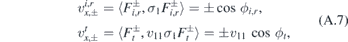
  for x > 0 and E − V > 0. The coefficients r and t can be found when taking into account conservation of energy, the momentum ky and conservation of probability current at x = 0. The calculation is straightforward and, for the sake of completeness, we present it in the appendix
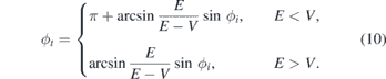
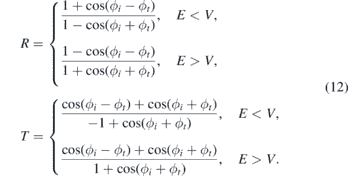
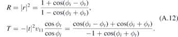
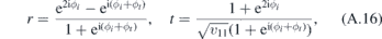
Taking into account that we have ϕi ∈ (−π/2, π/2), we can find the coefficients r and t as
The transmission and reflection amplitudes are
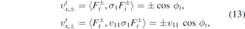
The velocity operators vx and vy can be computed as ![$\mathbf{v}=\frac{1}{i}\left[\mathbf{x},H\right]$](https://content.cld.iop.org/journals/0953-8984/32/29/295301/revision2/cmab7e5bieqn6.gif) , giving explicitly vx = v11(x)σ1 and vy = σ2. Their expectation values for the incident and the transmitted wave are
, giving explicitly vx = v11(x)σ1 and vy = σ2. Their expectation values for the incident and the transmitted wave are

A few comments are in order. First, one can see that there occurs unusual transmission for E < 0. Suppose that  and
and  and the incidence angle ϕi ranges between 0 and π/2. Then, taking into account ϕt ∈ (π/2, 3π/2), see (10), the velocity of the transmitted wave is
  and
and  . The fact that the
  has different sign then
  gives rise to the unusual transmission typical for metamaterials in optics and was utilized for design of Veselago lens in graphene [36]. Let us mention that classical particle with energy E > V and with the velocity
  would move along the trajectory y = v11 tan ϕtx + y0.
Now, let us consider the situation where the electrostatic potential V is small. Taking the limit V → 0 in the formulas (10), (11) and (12), we get (assuming that E > 0)

Hence, in the case of the vanishing potential term, the interface becomes completely transparent for particles of any energy and any incident angle. The total transmission T = 1 independent on the incident angle was discussed in [39] for specific values of energy. In the limit V → 0, the total transmission occurs for any angle and energy. Similarly to [39], it is marked by ϕi = ϕt. For x > 0, the trajectory of the particles changes to

We can write the wave function as
where  and
and  . The wave function
  satisfies the stationary equation

Hence, in the regime V(x) = 0 we can transform the model into the one of free particle. It provides a natural explanation for the fact that there is no backscattering on the interface as T = 1. Let us elaborate the link the free particle system in the next subsection in the context of general profiles of strain and v11(x).
2.2. Smooth strains and the free particle in disguise
We shall show that the Hamiltonian in (7) can be mapped to the free-particle energy operator for V(x) = 0. We suppose that the electrostatic potential induced by the deformation is compensated by the external electrostatic field. The Dirac equation for the free particle reads as

We define transformation of coordinates
and the operator
Then we have

The solutions of i∂tΦ(r, s, t) = H0Φ(r, s, t) transform as

It can be verified by direct calculation that the transformation preserves the norm,
It is worth noticing that the transformation discussed in [17] coincides with the one discussed here for γ = 0. By varying γ, we can adjust the angle of the incident wave Ψ(x, y, t) while keeping Φ(r, s, t) independent of γ. It is also worth noting that a similar transformation can be used to provide alternative explanation for Klein tunneling on the electrostatic barriers [42]. In our current case, it demonstrates that elimination of V(x) in (7) implies the total transmission T = 1.
To get further insight into the influence of the strain on the propagation of the Dirac fermions, we find it illustrative to consider the localized wave packets. Let us suppose that we have a localized (normalizable) function Φ(r, s, t) that satisfies i∂tΦ(r, s, t) = H0(r, s)Φ(r, s, t). Then we can get Ψ(x, y, t) that satisfies the Dirac equation of the strained system (23) and it is localized by construction. Now, let us suppose that the Gaussian-like wave packet Φ(r, s, t) propagates along the r axis (defined by s = 0) and disperses symmetrically with respect to the s axis. Then the wave packet Ψ(r, s, t) does no longer move along a straight line, but it rather follows the curve s(x, y) = 0 corresponding to

The relation (25) generalizes the formula (16) for the smoothly changing velocity v11(x).
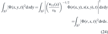
The change of trajectory is one effect that the wave packet Ψ(x, y, t) undergoes when passing through the strained region. The other one is its squeezing or stretching along x-axis. To see this, let us suppose that the probability density of the wave packet Φ(r, s, t) is practically zero outside a domain Ω(r, s, t). The domain changes its position and shape in time as the wave packet moves and disperses. We want to know how is the domain  where the wave packet Ψ(x, y, t) is localized. We have
Therefore, the wave packet Ψ(x, y, t) propagating in the strained material is confined in the deformed domain  . The change of the domain where the Dirac particle is localized is compensated by the term
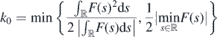
  that alters the probability density. For illustration, we can suppose that Ω(r, s, t) is a disc of radius ρ(t) centered7 in the maximum (r0(t), s0(t)) of the probability density of the wave packet. Then the deformed domain
  is composed from the points (x, y) such that
If v11(x) is constant on the domain where the wave packet is spread, the disk gets deformed into an ellipse,
When v11 < v0, we can see that the wave packet gets squeezed along the x axis. This way, the strain can focus the wave packets. In the figure 1, the focusing of the wave packet when passing through the region with v11(x) < v0 is depicted. As an approximation of Φ(r, s, t), we took the standard dispersing Gaussian wave packet.
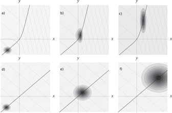
Figure 1. Focusing the probability density of a wave packet propagating through deformed crystal at three subsequent instants of time, (a) t = t1, (b) t = t2, (c) t = t3. For the illustration, we used v11 = v0(1 − μ(1 + tanh νx)). For comparison, the figures (d)–(f) in the lower row illustrate the evolution of the same wave packet in undeformed crystal at the same times. The thick dotted line is the trajectory along which the wave packet propagates. The dashed curves are defined by constant values of r whereas the dotted curves correspond to constant values of s, see (20). The wave packet was obtained by substitution of Φ(r, s, t) in (23) by a generic dispersing wave packet satisfying  .
.
Download figure:
Standard image High-resolution imageIn the rest of the section, let us discuss briefly the trajectory of the wave packet in dependence on several configurations of the strain u11(x) in more detail.
2.2.1. Asymptotically constant Fermi velocity
First, let us suppose that the Fermi velocity is asymptotically equal to v0 and the strain induces only a localized fluctuation of v11(x),

Deformation of this kind can be produced by folds of graphene sheet, see e.g. [12]. We suppose that the fluctuation Δv is small in the following sense,
Then the trajectory defined in (25) tends asymptotically to two straight lines

The two asymptotic trajectories yin and yout are parallel but mutually shifted. Therefore, the wave packet traveling along the trajectory (25) gets deflected by the mechanical deformation that gives rise to the inhomogeneous Fermi velocity (29). It is straightforward to compute explicitly the length of the normal vector n connecting the two lines,

see figure 2 for illustration.

Figure 2. Deflection of the wave packet by localized deformation. Probability density of a wave packet at two subsequent instants of time (a) t1 and (b) t2 (t1 < t2). For the illustration, we used  , 0 < μ < 1. The trajectory of the wave packet is determined by the two parallel lines yin and yout, see (31), that represent incoming and outgoing trajectories. The deflection is quantified by the distance of yin and yout measured by the vector n, see (32). The dotted curves correspond to constant values of s whereas the dashed curves are given by fixed values of r. Thick black dashed curve is the trajectory of the wave packet. In the illustration, we combined the generic dispersing Gaussian wave packet with the probability density
  with the formula (23).
Download figure:
Standard image High-resolution imageNow, we shall consider the situation where v11(x) tends asymptotically to two, possibly different, constant values. It can be induced by the unidirectional strain which vanishes for x → −∞ but it converges to a constant positive value for x → ∞. In this case, the displacement of the atoms in the crystal have linear-like growth for large values of x. We suppose that such a deformation can be achieved by the corresponding strain of the substrate on which the graphene sheet is positioned.
Let us suppose that the deformation should be such that the induced Fermi velocity satisfies

For these values of α, the O(x−α) term gives convergent contribution to the trajectory (25) of the wave packet so that y(x) can be written as

This type of deformation is illustrated in figure 1 where we fixed v11(x) = v0(1 − μ(1 + tanh νx)) for constant μ and ν.
2.2.2. Periodic fluctuation of Fermi velocity
Let us focus on the situation where the Fermi velocity is constant for all x < 0 and periodic for x ⩾ 0,
We suppose that the corresponding periodic strain can be achieved by the flexural modes [17] or by interaction with the substrate that gives rise to the Moire patterns [5]. Then the trajectory (25) can be written as
where [x] denotes integer part of x. In general, y(x) is no longer linear for x ⩾ 0. However, it can be confined between two parallel lines. Utilizing ![$x-1{\leqslant}\left[x\right]{\leqslant}x$](https://content.cld.iop.org/journals/0953-8984/32/29/295301/revision2/cmab7e5bieqn24.gif) together with positivity of v11(x), we get
together with positivity of v11(x), we get

where
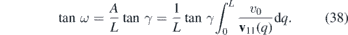
Hence, the periodic strain deflects the wave packet by the angle ω − γ. The deflection angle ω is just function of the incidence angle γ, periodicity L and the integral  so that it is the same for a family of Fermi velocities that share these quantities. It is worth noticing that ω also depends on the material constants β and a that stay hidden in definition of v11(x). There is no difference in propagation of the wave packets formed in the K and K' valleys.
3. Inhomogeneous unidirectional strains
In this section, we consider a system where the strain tensor and the Fermi velocity acquire the following forms
We suppose that u11, u22 and h are bounded and continuous and they are such that v11(x) and v22(y) are strictly positive. The stationary equation with the Hamiltonian (2) reads as
3.1. Focusing the wave packets
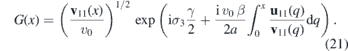
Before we proceed to the spectral analysis of the waveguides formed by the strains, let us make a brief comment on the influence of the strain on the wave packets. Likewise in the previous section, we can transform the Hamiltonian in order to eliminate the x-dependent potential and to simplify the kinetic term. Similarly to (20), we define transformation of coordinates
and the operator
Then we have

Here, the Hamiltonian with the flat Fermi velocity vij = v0ηij reads as
The solutions of i∂tΦ(r, s, t) = H0(r, s)Φ(r, s, t) transform as

Considering the transformation of coordinates (41), it can be rather complicated to get an explicit form of their inverse, x = x(r, s), y = y(r, s). Therefore, analytical calculation of Φ(r, s, t) together with the scattering characteristics can be impossible due to the complicated form of u11(x(r, s)) and u22(y(r, s)). However, we know how the wave packet Ψ(x, y, t) gets deformed in the regions where the Fermi velocity (39) fluctuates. The domain of its localization can be found in analogy with (26). For instance the circular domain  transforms into
  that is composed by
  ,
,  . If v11(x) ⩽ v0 and v22(y) ⩽ v0, the wave packet gets focused (the density of probability gets denser) by the strain.
3.2. Qualitative analysis of the waveguides
Let us focus on the ability of the strain to form a wave guide for Dirac fermions. We are no longer interested in the scattering but rather in the existence of localized (guided) modes in the strained region. We fix γ = 0 in (A.16) and we consider the electrostatic potential V(x, y) to be vanishing again. Then the stationary equation (44) gets the following form
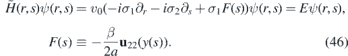
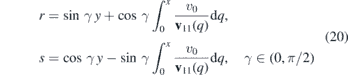
We require r and s to be mappings from  onto
onto  . They should be invertible, monotonic functions of x and y (there holds r'(x) ≠ 0 and s'(y) ≠ 0). The derivatives r'(x) as well as s'(y) should be bounded. For convenience, we fix

It is granted that there is also an inverse function y = y(s) that satisfies y(s(y)) = y.
We can take advantage of the translational invariance of the system and focus on subspaces with a conserved value of the momentum −i∂r. We make the partial Fourier transformation

The Hamitonian  can be rewritten as direct integral

The direct integral can be understood as a generalization of the partial wave decomposition for the case where the conserved quantum number is not discretized but acquires values from a real interval. As the potential term F(s) is bounded and continuous, the Hamiltonian Hk(s) is self-adjoint on the space of functions that are square integrable together with their first derivative.
We are interested in the configurations of mechanical strain where the Hamiltonian  possesses discrete energies. The reason is that these discrete energies give rise to discrete energy bands in the spectrum of
  and H(x, y) that can be associated with existence of (partially) dispersionless wave packets [43]. Indeed, let us suppose that we can find the solution of

where En(k) is a discrete energy of  labeled8 by n, i.e. ψk,n(s) is square integrable together with its first derivative. The intervals
  can be finite but also (semi-)infinite.
We can get eigenstates of H(x, y) from those of  ,
,
The discrete energies En(k) form discrete energy bands in the spectrum of the two-dimensional Hamiltonian, see figure 3 for illustration. We can use them to construct the following wave packets associated with the energy bands En(k),

This wave packet is normalizable provided that ρ(k) is normalizable (see appendix

The wave packet (52) has a remarkable property—it does not disperse along y axis. Indeed, there holds (again, see appendix for details)
where a and b are arbitrary real numbers, i.e. the probability density in the y direction is conserved during the time evolution.
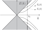
Figure 3. Spectrum of H(x, y). For fixed k0, we get energy spectrum of Hk(s) that consists of discrete energies (black dots) and the bands of positive and negative energies.
Download figure:
Standard image High-resolution imageThe speed of the wave packets can be approximated by the averaged group velocity
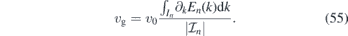
The spectrum of H(x, y) is symmetric with respect to 0. The transport of the wave packets (52) is bidirectional when ∂kEn(k) of the positive energy bands9 can be both positive and negative for  , see figure 4(a). When ∂kEn(k) of the positive energy bands is positive (negative) for all
  , the corresponding wave packets defined in (52) can move in one direction only, they are unidirectional, see figure 4(c). When the derivative of the positive energy bands has negative (positive) sign on a finite subinterval of
  and positive (negative, respectively) sign for all other
  , we say that the transport is essentially unidirectional, see figure 4(b).
Figure 4. Illustration of the spectrum of the system described by H(x, y). Discrete energy bands can be associated with the partially dispersionless wave packets (52) that are (a) unidirectional, (b) essentially unidirectional and (c) unidirectional. Below the energy graph, there are illustrations of the wave packets (52) composed from the states corresponding to the energies lying inside the dotted circles. The average group velocity of the wave packets vg is defined in (55).
Download figure:
Standard image High-resolution imageIt is worth noticing that the construction of the partially dispersionless wave packets is not limited to our model but can be applied to broad class of systems with translational symmetry, see [43] for more details. Examples can be found in the literature where explicit models were solved numerically. See e.g. [11–13, 44] for the discrete energy bands corresponding to the unidirectional, essentially unidirectional and bidirectional wave packets.
Explicit solutions of (51) are needed for construction of the wave packets (52). There are well known models where the stationary equation (51) is exactly solvable, let us mention the model with F(s) = tanh s. However, for reconstruction of the initial system described by H(x, y), we would need the explicit form of u22(y) (or v22(y)). It would be rather difficult to extract it from  . Nevertheless, there is one scenario where we can get a partial solution immediately. When

i.e. the strain along y axis is asymptotically constant. Then we can obtain the following zero modes for any fixed k

where one of them is vanishing exponentially for |x| → ∞ provided that (F− + k)(F+ + k) < 0. This way, we get the zero energy E0(k) = 0 of  . The wave packets (52) associated with this energy band do not move as its average group velocity would be identically zero.
3.2.1. Criteria for existence of the discrete energy bands
Instead of looking for exactly solvable configurations of (50), we focus on the qualitative spectral analysis of the system described by (46). It provides us with useful information on the energy bands En(k) without the need to solve the stationary equation. We will find the sufficient conditions for the strain such that it gives rise to waveguides supporting unidirectional or bidirectional transport.
Let us suppose that the second component of the strain tensor u22(y) is asymptotically constant, lim|y|→∞ u22(y) = 0. It implies that

We can utilize directly the results presented in [40, 41]. They are based on the fact that the square of  is Pauli-type diagonal Hamiltonian10,
  , with the spectrum bounded from below. It is possible to use the variational principle to find criteria for existence of its discrete energies. Existence of discrete energies of
  then implies existence of discrete energies in the spectrum of
  and also of the associated discrete energy bands in the spectrum of H(x, y). The corresponding eigenstates can be used in the construction of the dispersionless wave packets (51) and (52).
Let us summarize some of the relevant criteria below:
Let us suppose that F(s) is continuous together with its first derivative and  or there exists s0 such that F(s)(F(s) + 2k) ⩽ 0 for all s < s0. Then we can make the following conclusions [41]:
- (a)If F(s) ⩾ 0 (or F(s) ⩽ 0) for all
 , then there are no discrete energies in the spectrum of for all k ⩾ 0 (or for all k ⩽ 0, respectively).
 - (b)If, for some, (or if ), then there exists K > 0 such that for all k > K (or for all k < −K, respectively) there are discrete energies in the spectrum of .
- (c)If, for some, (or if ), then there exists K > 0 such that for all k > K (or for all k < −K, respectively) there are discrete energies in the spectrum of .
- (d)If F(s) ⩾ 0 and F(s) ≠ 0 then has discrete energies for all .
- (e)If F(s) ⩽ 0 and F(s) ≠ 0 then has discrete energies for all .


Suppose that F(s) is integrable.
- (f)If then there are discrete energy values in the spectrum of for all .
- (g)If then there are discrete energy values in the spectrum of for all .


A remark is in order. The criteria (b)–(g) represent sufficient conditions for existence of the discrete energies of  . It is possible that the discrete energy levels exist also outside of the specified interval for k. However, we do not have any tool how to guarantee their existence in that case. When F(s) ⩾ 0 (F(s) ⩽ 0), then (d) and (f) [or (e) and (g)] provide two different values for the threshold values of k. It is not possible to decide which one provides better estimate without evaluating them for an explicit F(s).
3.2.2. Waveguides for essentially unidirectional wave packets
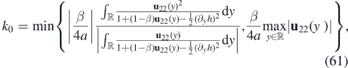
We can use these criteria to show that the deformation with

induces a waveguide for the essentially unidirectional wave packets (52). Let us suppose that  meets the assumptions of the criteria above. As u22(y) is positive, there holds F(s) ⩽ 0. Then it follows from (a) that there are no discrete energies in the spectrum of
  for any k ⩽ 0. We also know from (e) and (g) that there is a threshold
such that the effective Hamiltonian  has discrete energies for all k > k0. The value of k0 can be expressed in terms of u22(y) and the vertical displacement h = h(y) with the use of (41) in the following manner
We can conclude that whenever there holds u22(y) ⩾ 0 (but not identically u22 = 0), the strain induces a waveguide for essentially unidirectional transport of the dispersionless wave packets (52).
An inhomogeneous unidirectional strain is a good example of the deformation that gives rise to (60). The associated deformation vector is

where  is the strain and ν is the Poisson ratio11 gives rise to the following strain tensor and Fermi velocity
3.2.3. Waveguides for bidirectional wave packets
The waveguides formed by positive (negative) u22(y) for all  host essentially unidirectional wave packets. If we want to create waveguides that would host bidirectional transport, u22(y) has to acquire both positive and negative values. Revising the criteria (b) and (c), we can see that one way to create a waveguide for bidirectional wave packets is to have u22(y) ⩽ 0 for y ∈ (−∞, y0) and u22 ⩾ 0 for y ∈ (y1, ∞). The negative values of u22(y) mean that the atoms from the lattice have to get closer together. It is worth mentioning that free standing graphene is stable for small values of compressive strain only. When the compression exceeds the threshold value of ∼0.1%, the strain gets compensated by creation of folds [45]. Hence, the experimental formation of waveguides for bidirectional wave packets by compressive strain could be a rather complicated task.
3.2.4. Waveguides for valleytronics
Let us suppose that strained graphene with Fermi velocity (39) is in presence of an external magnetic field perpendicular to the crystal, B = (0, 0, ∂yAx(y)). Contrary to the pseudo-magnetic gauge field induced by the mechanical deformations, the magnetic field breaks the time-reversal symmetry and comes with opposite sign when we consider Dirac fermions in the vicinity of the second Dirac point K' ≡ −K. The Dirac Hamiltonians at the Dirac points K and −K can be written in the following form
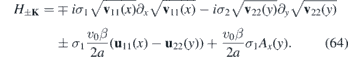
Let us set the strain and the magnetic field such that

Then we follow the steps (46)–(49) for both H±K and get the effective one dimensional operators


Therefore, the Dirac fermions at the vicinity of the Dirac point K are effectively governed by free-particle Hamiltonian which has no discrete energies in its spectrum. On the other hand, the Dirac fermions at the Dirac point K' are subject to the vector potential  that can induce discrete energies. In particular, when u22 ⩾ 0, the strain forms waveguide for essentially unidirectional wave packets in the K'-valley and the spectrum of H−K looks like figures 4(b) or (c). The combination of the strain and the magnetic field does not confine Dirac fermions in the K-valley. When the condition (65) for the perfect valley polarization is not met, there can be discrete energy bands both in the spectrum of HK and H−K. However, their number goes to zero as the effective vector potential gets small in the corresponding valley. The combination of the external magnetic field with the strain in order to control propagation of the electrons in K and K' valleys appeared e.g. in construction of valley filters [10, 33, 46]. Valley currents in the nanoribbons induced by unidirectional strain were analyzed in [47].
In the end of the section, let us make few comments. The qualitative approach to the spectral analysis was based on the results obtained via standard variational principle. It was applied on the square on the effective Hamiltonian (49) that coincides with Pauli Hamiltonian [40]. If the electrostatic field was included, this approach would be no longer feasible as the square of the effective Hamiltonian acquires more complicated form. Nevertheless, it should be possible to study the influence of the small V(x) on the discrete energy bands of H(x, y) perturbatively, with the use of the test functions that provide estimates of the ground state energy of  , see [40] for more information.
4. Conclusion
In the article, we focused on the systems described by two-dimensional Dirac equation where the Fermi velocity is diagonal and inhomogeneous. In the section 2, we showed that the inhomogeneous Fermi velocity (6) gives rise to deflection and focusing of the incoming wave packets, see figure 1. The shifted trajectory as well as the deflection angle can be found explicitly (32) and (38). The key ingredient was the mapping (23) between the deformed equation (7) with V(x) = 0 and the free-particle system. The considered effect belongs to family of phenomena where the scattered and transmitted electrons behave in analogy with optical systems [10, 32–36, 38, 39]. In particular, we extended the results on the super-diverging lens [39] where deflection was discussed in the model with piece-wise constant Fermi velocity.
It is worth mentioning that similar transformation was discussed in [42] where it was used to explain the absence of backscattering of Dirac fermions on the impurities in carbon nanotubes or on electrostatic barriers. In non-relativistic quantum mechanics, the perfect transmission in the Pöschl–Teller reflectionless system is explained by the Darboux transformation that relates the Pöschl–Teller Hamiltonian with the free particle one [48].
In the section 3, we discussed how deformations represented by the strain tensor (39) can induce waveguides for partially dispersionless wave packets (52). We used the results of qualitative spectral analysis [40, 41]. The wave packets (52) associated with the discrete energy bands can have major influence on the conduction of the waveguide as they do not disperse rapidly outwards the wave guide during time evolution. We found that any nonvanishing deformation (39) with u22 ⩾ 0 gives rise to the wave guide for the essentially unidirectional wave packets. Our results are complementary to the existing literature where explicit models were considered. Guided modes in the waveguides induced by inhomogeneous Fermi velocity were discussed e.g. in [49–52] with Fermi velocity fixed as v = v(x)η. In [12, 53], the Fermi velocity was associated with the applied strain. These models differ from our one by presence of external fields (typically electric potential) or by the Fermi velocity that appears in the Hamiltonian without the associated pseudo-magnetic vector potential (4).
Finally, let us notice that despite we supposed the Dirac fermion to move in graphene throughout the work, there is an expanding family of Dirac materials where dynamics of low-energy particles is described by the same equations [20, 21, 54, 55]. This broadens the applicability of the obtained results to a wider class of physical systems.
Acknowledgments
V J was supported by GAČR Grant no.19-07117S.
Appendix A.: The model with the step-like strain
We shall find solutions of the following equation
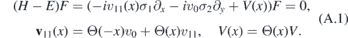
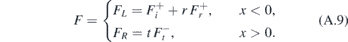
We set v0= 1. It is convenient to write the solutions separately for x < 0 and x > 0. We denote Fi,r,t the incident, reflected and transmitted waves,
Here Θ(x) is the Heaviside step function and the factor  stays for normalization over a unit volume. The states satisfy

We should find how ϕr and ϕt depend on ϕi and what are transmission and reflection coefficients/amplitudes. We will get it from the conservation of energy, of the momentum ky and from the conservation of probability current at the interface x = 0. We will suppose that E > 0. It is convenient to consider the cases E − V < 0 and E − V > 0 separately.
First, we discuss that case where E − V < 0. The conservation of energy dictates

We can parametrize
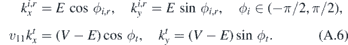
For x < 0, the kinetic energy is positive so that we deal with  while it is negative for x > 0, i.e. the transmitted wave corresponds to
  . The operators vx and vy corresponding to the velocity along x and y axis can be found as
 ![$\mathbf{v}=\frac{1}{i}\left[\mathbf{x},H\right]$](https://content.cld.iop.org/journals/0953-8984/32/29/295301/revision2/cmab7e5bieqn81.gif) , v = (v11(x)σ1, σ2). The expectation value of the velocity is independent on the energy,
, v = (v11(x)σ1, σ2). The expectation value of the velocity is independent on the energy,

Notice that velocity and momentum differ in sign for the transmitted waves. The particle of energy E > 0 that comes from the left and passes through the interface has  which implies that ϕt ∈ (π/2, 3π/2). Therefore, we can define ϕ2 = ϕt + π, ϕ2 ∈ (−π/2, π/2). The conservation of the momentum ky implies (V − E) sin(ϕ2 + π) = E sin ϕi and
  .
.
Now, let us focus on the relation between ϕi and ϕr. We know that  as it corresponds to the velocity of particle reflected from the interface. Together with
  and
and  we get sin ϕi = sin ϕr, cos ϕr = −cos ϕi. The two relations can be satisfied provided that ϕr = π − ϕi.
The wave function scattered on the interface has the following form
The coefficients t and r can be found from the conservation of probability current at the interface. The current operator in the x-direction is jx = v11(x)σ1. We have  that can be satisfied as long as

It provides us with the following relations
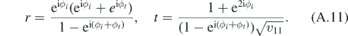
The reflection and transmission amplitudes can be found from the relation of probability current conservation, 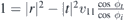 . From this relation, we can identify transmission and reflection amplitudes
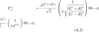
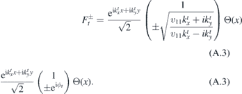
Now, let us turn our attention to the case where E − V > 0. We have

We can use the same parametrization for  as in (A.6). For the transmitted wave, we have

To find the relation between ϕi and ϕr,t, we can follow the same steps as above. The only difference comes from the fact that the transmitted wave is described by  , i.e. the velocity
  has the same direction as
  . We get the following relations

Condition on the continuity of probability current of the wave function  at the interface gives us the following values of the r and t
as well as of the reflection and transmission coefficients
Appendix B.: Properties of the dispersionless wave packets
The norm of the wave packet (52) is given by the coefficient function ρ.
On the last line, we used the fact that the Fourier transform is a unitary mapping and ψk(s) is a normalized bound state of  .
.
The wave packets (52) do not disperse in y direction. In what follows, we do not write the label of the energy band explicitly, E(k) ≡ En(k),  , ρ(k) ≡ ρn(k), ψk(s) ≡ ψn,k(s). The probability of finding the particle in the interval y ∈ (a, b) at time t can be calculated as
where we used unitarity of the Fourier transform on the third line. We can see that it does not change in time. Since a and b are arbitrary, we can conclude that the probability of finding the particle in a fixed interval of the y axis does not change intime.
Footnotes
- 6
∂1 ≡ ∂x, ∂2 ≡ ∂y.
- 7
- 8
We label just the positive energies as the spectrum is symmetric with respect to zero.
- 9
The negative energy bands has opposite sign of derivative so that the corresponding wave packets move in opposite direction. However, as they are composed of holes, they contribute to the same direction of electric current.
- 10
- 11
The homogeneous unidirectional strain corresponds to f(X) = x.
