1. Introduction
Wavefront shaping techniques are nowadays instrumental in controlling light propagation through complex media, including highly scattering, optically turbid, and other light randomising environments [
1,
2,
3,
4,
5]. An exemplar optically complex media is a multi-mode optical fibre (MMF), which can support a large number of modes propagating at different group velocities. Despite the somewhat elaborate process of imaging through MMFs, their popularity in in vivo holographic microendoscopy is increasing due to their minuscule dimensions (≈100 µm in diameter), resulting in minimal damage to sensitive tissue, while allowing highly detailed observations (with spatial resolution better than a µm) [
6].
The technological complexity of MMF-based imaging approaches is derived from a strong contrast between light transport through a MMF and that of imaging devices designed to retrieve an object’s image across a given optical plane. Any single-frequency light field (e.g., laser focus, spherical or plane wave, or an image of an object illuminated by laser light) coupled into such a fibre gets decomposed into a set of orthogonal fibre modes which will acquire disparate phase shifts while propagating through the fibre medium. Even after propagating only a fraction of a millimetre through a typical MMF, the output field will bear no resemblance to the input field; instead taking the shape of an apparently randomised speckled structure (see inset in
Figure 1). The phase shifts depend strongly on the dimensions, materials, length, curvature, and environmental conditions (temperature, mechanical stress) of the fibre, moreover, even minute deviations from the ideal refractive index profile are responsible for significant phase changes. Thus, only when all of these factors are known with a very high accuracy can such a complex optical system lend itself to numerical predictions that agree with experimental observations [
7].
Despite these constrains, coherent light signals propagate through complex media in a deterministic manner. Therefore, in cases where optical geometries comprising stationary optical fibres are considered, light transport can be characterised by experimental assessment or calibration. There are several calibration methods available, e.g., single-pulse acquisition [
8], machine-learning [
9], or referenceless techniques [
10,
11]. However, the direct interferometric approach using a reference signal arguably provides images with the highest purity [
12,
13]. To carry out the calibration procedure,
N input optical modes,
, forming a convenient (preferably orthogonal) basis are created and sequentially coupled into the MMF using a spatial light modulator (SLM). The resulting output optical field across the fibre facet, or other desired plane, is recorded using a CCD camera. We use phase shifting interferometry to retrieve both phase and amplitude [
14,
15], which work also with the reference co-propagating through the fibre. The output field can then be expressed as a superposition of conveniently chosen output modes
. The light transport process through the MMF is then represented as a
transmission matrix (TM) with elements
:
where
p is the polarization state,
is the phase, and
A is the amplitude of the complex element
connecting the
i-th input mode to
j-th output mode of the optical field. The circular polarisation is almost perfectly preserved in the optical fibre, as was shown in [
7]. Therefore, we have decided to use only one circular polarisation state in these experiments to reduce complexity of the apparatus—the
p index is thus omitted and
is used in the rest of the text. There are two basis sets commonly used in TM measurements of random media: A set of spatially independent hologram areas in the SLM plane and a set of equidistantly separated diffraction limited spots at the proximal end of the fibre. In this study, we have chosen the latter as our input modes. The main advantage of such an input mode base is its power efficiency, because the whole input beam profile takes part in the creation of each input mode. The output modes can be conveniently represented by digital camera pixels in the output image plane. Here we discuss how the calibration can be implemented to achieve a homogeneous illumination of the field-of-view (that is homogeneity of the intensity of the output modes) and thus enhance imaging quality.
The most accurate techniques so far use a spatially filtered external reference beam. Free-space reference optical set-ups are generally prone to air movement and temperature changes, and bulky optics are required to shape the laser beam profile to achieve the desired optical landscape. It is also possible to use a single mode optical fibre (SMF) for guiding the reference beam, but the SMF introduces additional sensitivity to temperature and mechanical noise affecting the reference’s output phase. To overcome the phase fluctuations, it is necessary to track this offset using a feedback loop to obtain high quality TMs, adding another level of complexity to both optical path and calibration procedure. These detrimental effects can be minimised if a common path interferometry set-up is employed. In this approach, input modes to the MMF are used to generate both reference and probe waves, which then co-propagate through the MMF. Such a configuration decreases the complexity of the optical apparatus and the difficulty of the adjustment procedures. Nonetheless, other unwanted effects have to be dealt with. Mainly, due to the speckled nature of the output intensity pattern generated by an input mode propagating through a MMF, the internally guided reference wave would not have enough intensity in certain areas at the distal plane to obtain any reasonable information with a phase-shifting technique for all of the input modes resulting in “blind spots” in the TM [
16]. Several approaches were presented to solve this issue. Bianchi et al. suggested measuring several TMs with different internal references and using the input mode phase offset from the TM with a maximal signal for a given output mode [
17]. This approach, however, leads to an uneven image reconstruction performance given that the efficiency for each reference is not uniform. Another approach involves taking advantage of the memory effect in turbid media and covering the blind spots using bright neighbouring output modes translated by a tilted wave front [
18]. Since the memory effect is limited using thicker or more diffusing samples, the work [
18] also suggests employing additional TM measurements with internal references using plane wave and waves modulated with spiral phase masks and opposite topological charges (+1, 0, and –1) yielding complementary bright and blind spots. The final TM is again given by a combination of the most reliable speckles from the measurement with all three internal references. Our suggested method, however, uses combined signals from several measurements employing different references so that the totality of the output modes can be retrieved using complementary information. One may expect that the number of blind spots grows proportionally to the number of guided modes, so the required number of internal references might be higher for optical fibres with larger V numbers.
2. Materials and Methods
In the proposed experimental technique, we used a Cartesian array of non-overlapping focal spots as the input mode basis and a sensor array (CCD) in the image plane as the output modes of the system. The input modes were addressed individually by displaying the appropriate hologram on a phase-only SLM. We treat the light field complex until synthesising the hologram accordingly to [
16], so both phases and intensities of the input modes are addressed this way. The output mode intensities were acquired simultaneously with a digital CCD camera. A randomly chosen input mode was used as an internal reference wave for the calibration procedure. The measured input mode was addressed and phase shifted on the SLM in a range of
with
steps and the intensity on every camera pixels was recorded to calculate the amplitude and obtain the phase difference between the probe and reference modes
[
15]. In principle, three phase shifts suffice to recover the phase offset of a particular mode. Yet, in our experience, using two periods with four steps, i.e., eight steps total, is better than signal averaging and yields a reduction in measurement noise [
19].
We observed that the resulting output mode intensity homogeneity is enhanced when information from all the single-reference TMs is added together and weighted by the amplitude
. To find the phase difference between the references,
r, and for the
j-th output mode,
, we calculate a dot product of
j-th TM columns:
The resulting output mode vector is then given by a sum:
where
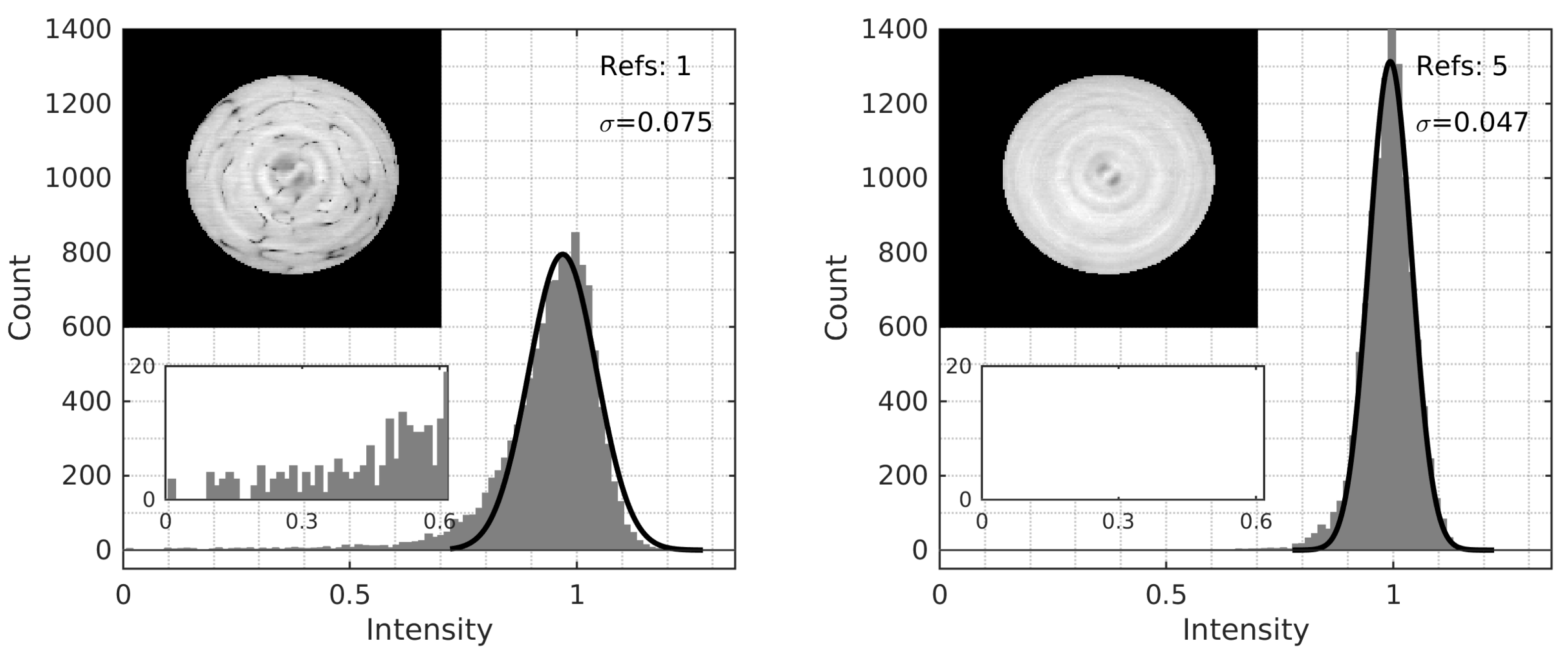
R is the number of internal references. Combining each single reference TM of every output mode in this manner results in the final TM with suppressed blind spot areas, as demonstrated in
Figure 2.
The experimental apparatus was built with a near-infrared fibre laser, IPG YLM-10-LP-SC, emitting a linearly polarised light beam with a wavelength of nm. The output beam is expanded using achromatic doublet lenses to fully cover the phase grating created on the SLM (HSP1064-512-PCIe, Meadowlark Optics, Frederick, CO, USA). The SLM is based on liquid crystals and imparts a phase shift on the reflected beam in the range of 0–2, higher phase shifts must be therefore wrapped in this interval. Switching between phase holograms is possible at a maximum refresh rate of 100 Hz. The zeroth and higher orders of diffracted light are filtered out with an iris aperture. The linear polarisation of the laser beam is changed to circular with a plate. The phase mask, shifted to the first diffraction order, is imaged onto the back focal plane of a microscope objective (PlanCN 10/0.25, Olympus, Tokyo, Japan) and projected on the input facet of the MMF (Thorlabs FG050LGA, NA 0.22, diameter 50 µm). The pattern on the output fibre facet is imaged using an identical microscope objective and tube lens to a fast CMOS camera (acA640-120uc, Basler, Ahrensburg, Germany) through another plate to change the polarisation back to linear.
The FG050LGA MMF has approximately 260 propagating modes in each orthogonal polarisation state involved in image transmission. A total of 525 input modes were projected on the proximal end of the fibre and approximately 15,000 output modes were analysed on the detector side of the set up. The number of input modes is higher than the number of guided modes, the measurement configuration is therefore oversampled and fully describes the transmission of the system.
The results of this approach strongly depend on the number and position of the internal references. To visualise this dependence, all output modes were addressed successively and their intensity was acquired with the respective pixels on the CMOS chip calibrated for a linear response. The recorded values were put together in one image and uniformity was expressed using the interference contrast formula:
3. Results and Discussion
In order to evaluate the uniformity of the intensity (of the generated foci used for imaging) across the field of view, we created transmission matrices based on different choices of references, measured the intensity of the resulting foci, and calculated the parameter
U (Equation (
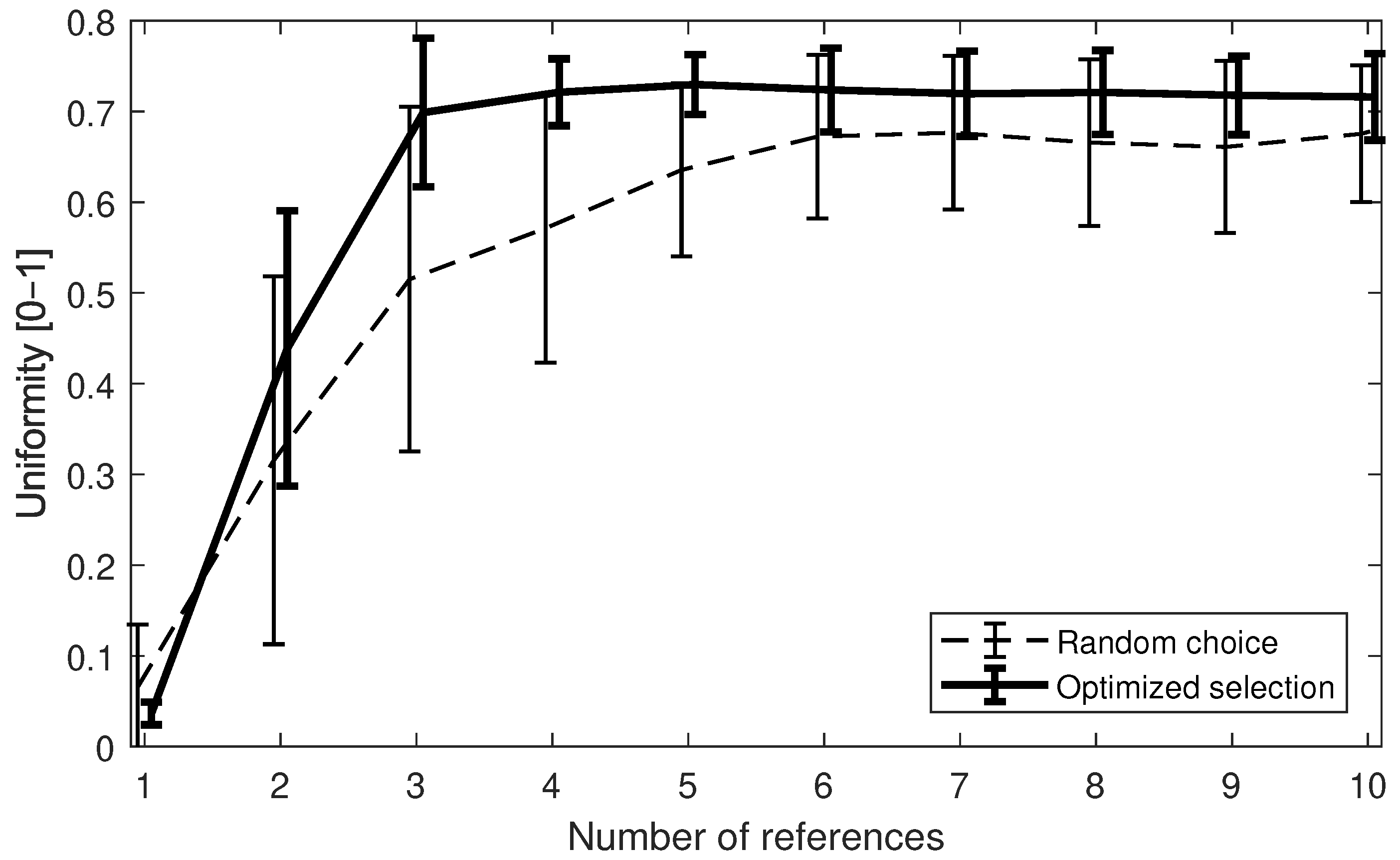
4)). More than 60 measurements each with 10 randomly chosen internal references were performed. After that, every measurement was analysed using sets of 1–10 single-reference TMs randomly selected from the measured data (i.e., more than 600 recordings of output modes intensities). Since each of these uniformity checks was based on a different set, the resulting graph has a sizeable variation coefficient. Nonetheless, the trend shows that using more than three internal references is desirable and acquiring more than 6 does not have an appreciable impact on the quality of endoscopic imaging. We speculate that 5 randomly chosen internal references, in most cases, are ideal. It is possible to optimise the procedure. First, all the input modes are projected through the fibre and their corresponding intensity pattern is recorded. After that, all the patterns are binarised with a threshold and the base reference (i.e., the input mode with the best coverage of the output) is selected. Finally, the other patterns are successively compared with the base to find the optimal combination with the best mutual coverage of blind spots. These are selected as internal references for the TM measurement. The resulting combination gives much faster convergence to homogeneous distribution of the output modes’ intensity than random selection of the reference waves. See
Figure 3 for a comparison of a random and optimised reference choice. An example comparing the output mode intensity obtained using 1 and 5 internal references is presented in
Figure 2 together with a histogram of intensity values. There are no blind spots, but a shady “coffee bean”-shaped artefact can be noticed in the central area of the MMF core. This effect is caused by a slight irregularity of the waveguide’s cylindrical shape causing leakage between the circular polarisation states. The artefact vanishes if TMs obtained for both orthogonal polarisation states are used, as can be seen in previous work [
16]. Furthermore,
Figure 2 also shows the intensities obtained for 5 internal references are more tightly centered around the average value leading to a 40% decrease of the standard deviation
.
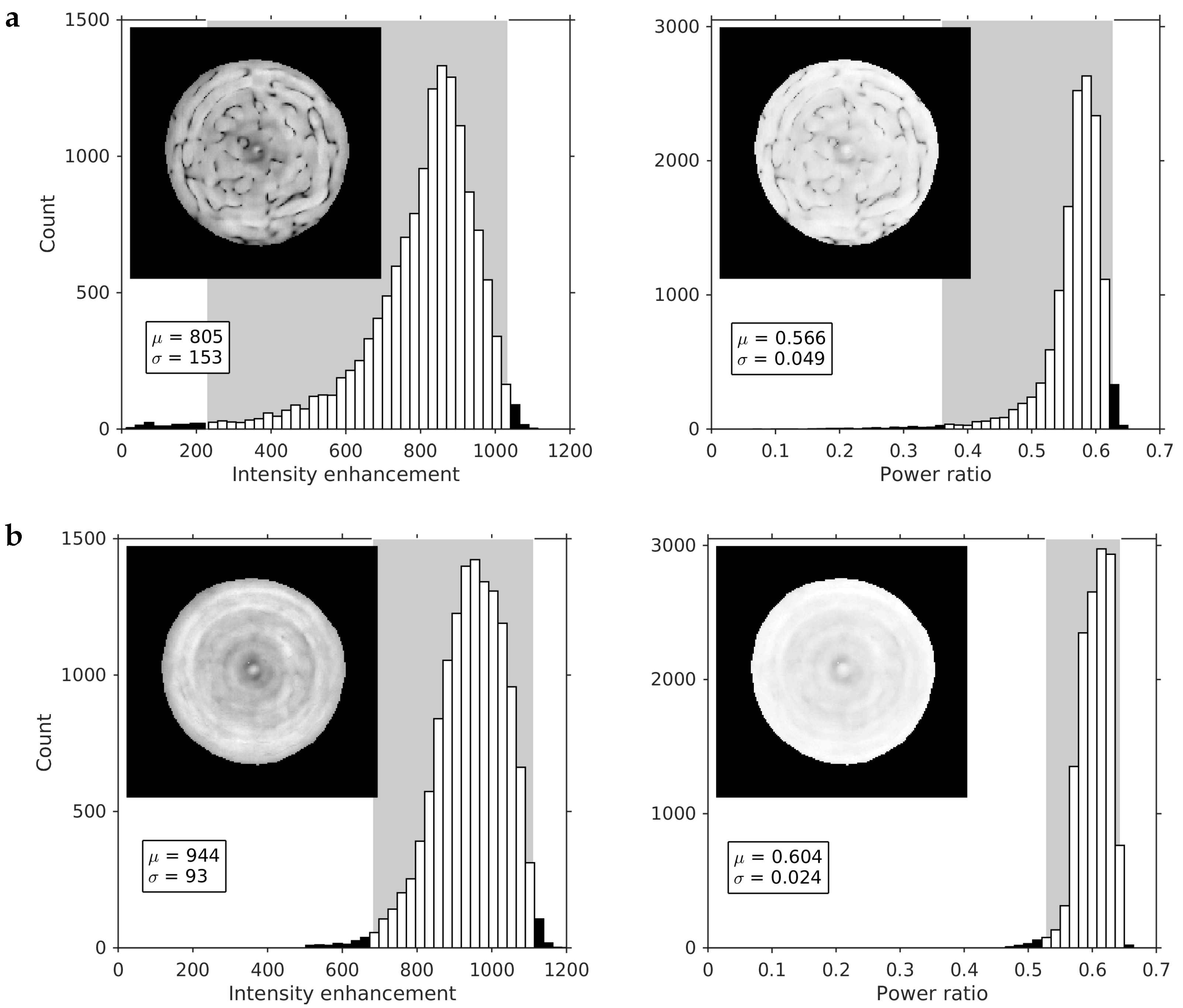
For imaging applications such as fluorescence scanning endoscopy, it is important to have a uniform ratio between the optical power contained in the scanning point and the optical power distributed across the rest of the field of view. A higher intensity enhancement, i.e., ratio of the peak to the average background intensity, also improves image quality. Both of these properties were obtained using high dynamic range imaging (HDR) of the output foci. The HDR images of each output foci were acquired using 8 different exposition times so that both peak and background intensities could be represented with sufficient resolution(see
Figure 4). In the ideal case, each of generated foci (output modes) is a diffraction limited spot with a profile described by the Airy disc [
20]. Therefore, we fitted measured intensity of the
j-th output mode with an Airy disc, using the following equation:
and
are the Airy disc peak and average background intensities, respectively. Furthermore,
is the Bessel function of the first order, and
,
,
, and
are coordinates of the disc center and its widths in
x and
y directions, respectively. The enhancement factor
and power ratio
are obtained from the fitted parameters as follows:
where
is the intensity profile of ideal Airy profile described by Equation (
5) and
is the measured intensity.
Figure 4 shows the change of the enhancement factor and power ratio between the cases of 1 and 5 internal references. For both quantities, we can see an increase of the mean value value and narrowing the histogram width, i.e., decrease of the standard deviation. This confirms that the blind spots (also seen in the intensity maps in
Figure 4) are completely eliminated by combination of multiple internal references.
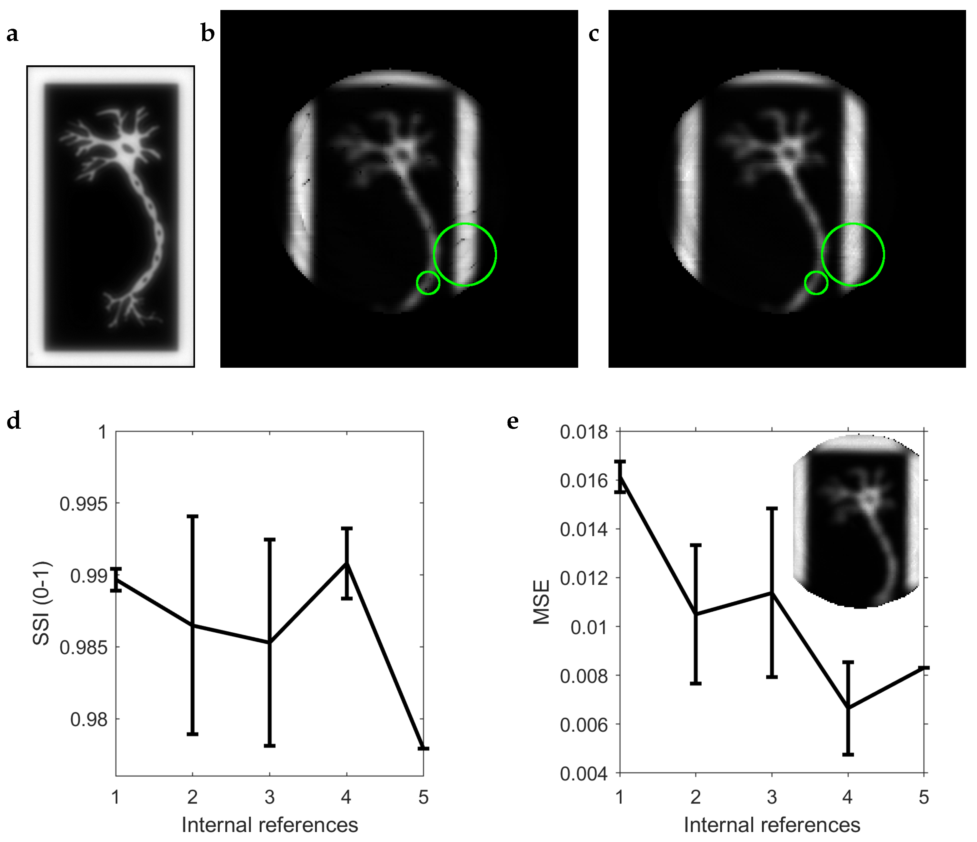
To test imaging with multiple internal references, the endoscope was used in a transmission regime. Output modes were addressed sequentially to scan the field of view. To mimic the detection approach used in scanning microscopy techniques, e.g., fluorescence imaging, the sum of the intensity of all the camera pixels was recorded, effectively turning the camera into a bucket detector. The imaging target was prepared using electron beam lithography to etch, in a thin molybdenum layer, the image of a neuron as a binary mask. A microscope cover-slip was used as a substrate (see
Figure 5). The lateral resolution of the NIR MMF endoscope was
µm. In contrast, the bright-field microscopy image obtained using planachromat objective Olympus 20×/0.4 has a resolution of
µm (see
Figure 5a). The blind spots in TM calibrated with 1 internal reference can clearly be recognised in the image (see
Figure 5b), while using a TM from a calibration with 5 random references results in a much better image, with fewer dark regions (see
Figure 5c). To evaluate the imaging performance affected by blind spots with respect to human vision perception, 5 internal references were selected using the optimisation procedure and used to record the sample. The images of the neuron mask were compared to a ground truth image by structural similarity index (SSI) [
21]. The ground-truth image prepared as an average of measurements taken with 3 and more internal references is shown as the inset of
Figure 5e. The mean SSI of the 5 image series together with its error bars (see
Figure 5d) shows a value of SSI close to 0.97–0.99 for all cases with 1–5 internal references. This means that the visual perception of the endoscopic image is not considerably improved by adding multiple references and that the “blind spots” in the image go mostly unnoticed by humans. To evaluate the imaging performance affected by blind spots quantitatively, we compared the images of the neuron mask and the ground truth image by the mean squared error (MSE) similarly to our previous work [
22]. Both the measured image as well as the ground truth image were standardised to the zero mean and the unit standard deviation prior MSE calculation in order to compensate for drifts in overall intensities.
Figure 5e shows the average MSE as a function of the internal reference count. MSE decreases with the increasing number of internal references, in agreement with the results shown in
Figure 3.
The overall time of calibration increases with the number of internal references used during the process. As the frequency of liquid crystal-based SLMs is in higher tens of Hz, this delay might be a constraint e.g., during in vivo imaging, where short re-calibration times are necessary. However, with binary phase SLMs [
23,
24] or MEMS-based devices for wave-front shaping, like DLP/DMD instruments [
19], capable of achieving refresh rates of tens of kHz, this increase in calibration time becomes negligible.
4. Conclusions
In conclusion, using internal, rather than external, references to calibrate a MMF endoscope leads to a more compact apparatus that require fewer optical elements and, consequentially, a higher stability of the experimental system. Furthermore, the sensitivity to phase fluctuations is reduced since the reference and signal beams have a common optical path. The trade-off for this stability is the necessity for multiple calibration steps using different references, in order to overcome the blind-spots caused by the speckled nature of the internal reference, resulting in an increase of the calibration time. We, however, show that with an optimised choice of reference, only 2–3 references are required to obtain a transmission matrix, resulting in a high image quality.

 ,
, 


