Review

Computational Fluid Dynamics Modelling of Liquid–Solid Slurry Flows in Pipelines: State-of-the-Art and Future Perspectives

by
Gianandrea Vittorio Messa
1,*,
Qi Yang
1,
Oluwaseun Ezekiel Adedeji
2,
Zdeněk Chára
3,
Carlos Antonio Ribeiro Duarte
4,
Václav Matoušek
3,
Maria Graça Rasteiro
5,
R. Sean Sanders
2,
Rui C. Silva
5 and
Francisco José de Souza
6
1
Department of Civil and Environmental Engineering, Politecnico di Milano, 20133 Milano, Italy
2
Department of Chemical and Materials Engineering, University of Alberta, Edmonton, AB T6G 1H9, Canada
3
The Czech Academy of Sciences, Institute of Hydrodynamics, Pod Pat’ankou 30/5, 166 12 Prague, Czech Republic
4
Department of Engineering, Federal University of Catalão, Catalão 75704-020, Brazil
5
Department of Chemical Engineering, CIEPQPF, University of Coimbra, 3030-790 Coimbra, Portugal
6
School of Mechanical Engineering, Federal University of Uberlândia, Uberlândia 38400-902, Brazil
*
Author to whom correspondence should be addressed.
Processes 2021, 9(9), 1566; https://doi.org/10.3390/pr9091566
Submission received: 26 July 2021 / Revised: 27 August 2021 / Accepted: 28 August 2021 / Published: 1 September 2021
(This article belongs to the Section Process Control and Monitoring)

Abstract

:
Slurry pipe transport has directed the efforts of researchers for decades, not only for the practical impact of this problem, but also for the challenges in understanding and modelling the complex phenomena involved. The increase in computer power and the diffusion of multipurpose codes based on Computational Fluid Dynamics (CFD) have opened up the opportunity to gather information on slurry pipe flows at the local level, in contrast with the traditional approaches of simplified theoretical modelling which are mainly based on a macroscopic description of the flow. This review paper discusses the potential of CFD for simulating slurry pipe flows. A comprehensive description of the modelling methods will be presented, followed by an overview of significant publications on the topic. However, the main focus will be the assessment of the potential and the challenges of the CFD approach, underlying the essential interplay between CFD simulations and experiments, discussing the main sources of uncertainty of CFD models, and evaluating existing models based on their interpretative or predictive capacity. This work aims at providing a solid ground for students, academics, and professional engineers dealing with slurry pipe transport, but it will also provide a methodological approach that goes beyond the specific application.

1. Introduction

1.1. Engineering Aspects and Physical Features of Slurry Pipe Transport

Hydraulic transport of solid particles in the flow of carrying liquid is of great importance in many industries, including mining, dredging, oil and gas, chemistry, agriculture or waste treatment [1,2,3,4,5]. In those applications, it can pose a reliable, safe, economic and environmental-friendly alternative to other means of transportation as for instance trucks.
The broad variety of environments in which the solids hydrotransport is applied produces different solid–liquid mixtures to be pumped and conveyed primarily through pressurized pipes. Water is typically the carrying liquid but the carried solids can be very different from very fine to very coarse and from very heavy to very light. The two phases (liquid and solid) interact with each other while flowing in a conduit and significantly affect the behavior of the mixture flow. This paper discusses transport in pressurized pipes and focuses on turbulent flows of mixtures (slurries) composed of Newtonian carrier and particles coarse and/or heavy enough to alter the internal structure of the flow by causing an asymmetrical distribution of velocity and non-uniform distribution of solids in the cross section of a pipe. In such flows, called settling slurry flows, the solid particles interact with turbulent eddies of the flowing carrier and may also interact with each other through interparticle collisions or longer-lasting contacts [6,7,8].
Essentially, there are three basic types of settling slurry flow. At one extreme is the pseudo-homogeneous regime, typical of flows laden with fine particles (typically fine sand of particle sizes between 60 and 200 microns) flowing at high velocity. Their submerged weight is carried by fluid support mechanisms associated with flow turbulence. The distribution of suspended particles is close to uniform although some gradient usually occurs in the pipe cross section, see Figure 1a. Viscous friction is responsible for flow energy loss. The other limiting case is represented by the fully-stratified regime, typical of flow conveying large, rapidly-settling particles at low velocity. Their submerged weight cannot be carried by flow turbulence and they travel in the lower part of the pipe by saltation, or as a sliding bed (Figure 1c). Particle contacts with each other and with a pipe wall considerably contribute to the overall flow friction. The intermediate case, for which both inter-granular contact and fluid support mechanisms are significant, is called heterogeneous flow (Figure 1b). For relatively large particles, the heterogeneous flow regime can be more distinctly stratified with a detectable sliding bed and the transported grains can be supported either by turbulent eddies or by mutual collisions above the sliding bed. Additionally, often encountered in practice is the flow of broadly graded solids in a Newtonian carrier in which particles of quite different sizes and supported by different mechanisms interact with each other. Overall, the behavior of the discussed slurry flows is quite complex as it is a result of the number of different mechanisms governing the flow and being responsible for particle support and friction.
Settling slurries tend to stratify in the pipeline and the degree of stratification affects both the pipeline resistance and transport safety. Typically, the pipeline resistance is quantified by the frictional pressure drop over the length of the pipe, whereas the transport safety is evaluated by the flow velocity, which must exceed the minimum safe velocity at which the system should operate without the danger of accumulation of particles in the form of a deposit at the bottom of the pipe which may result in pipe blockage. The operating velocity at which first grains stop moving and start to form the deposit is called the deposition-limit velocity and it is one of the key parameters in a description of slurry flow for purposes of design or operation of a slurry transport system typically composed of a pipeline and a pump [9,10].
Additional quantities essential to evaluate and quantify the production and efficiency of the slurry transport system include those describing properties of slurry and of the slurry flow. Regarding the production, the solids are normally the “payload” while the conveying liquid is only the “vehicle”. Hence, the volumetric flow rate of solids Q s is an important parameter and it is related to the total volumetric flow rate of mixture Q m through the delivered solids concentration C vd , which is defined as the ratio of the two flow rates. This concentration usually differs from the average spatial volumetric concentration C vi of solids in a flow cross section. C vi tends to be higher than C vd due to the lag of the solid phase in the slurry flow and the difference in values of the two concentrations depends primarily on the degree of flow stratification.
The transport efficiency is appropriately quantified by the specific energy consumption (SEC), which is a measure of the energy required to move a given quantity of product over a given distance. It is directly proportional to the hydraulic gradient, i m , which represents in the dimensionless form the drop of static pressure due to friction in the slurry flow along the unit length of the pipe. The SEC is a ratio of i m , and C vd , for solids of certain relative density S p , that is, the ratio between the density of the solid particles ρ p and the density of the carrier liquid ρ l .
The lower the SEC, the more energy-effective the pipeline transport is [11]. It follows from the definition of SEC that the basic requirements, for minimum energy consumption, are an optimally large value of C vd , together with operation at the velocity near the minimum value of i m . This minimum can be found on the pipe characteristic curve showing the relation between i m and the flow velocity V m for slurry at a constant concentration C vi . (Figure 2).

1.2. Modeling of Slurry Pipe Flows

Predictive models are essential design tools for slurry transport systems. In this perspective, the prediction of the pipe characteristic curve is one of the key tasks of slurry flow modelling, and another major task is to predict the deposition-limit velocity, V dl , which is the value of flow velocity below which solid deposit is observed. A more detailed prediction of slurry flow includes information on the internal structure of the flow in the form of distributions of local velocity and concentration (e.g., [13]) which helps to understand the friction and to predict other phenomena, such as the erosive wear of a pipe wall.
There are several sorts of models available for predictions of the slurry flow quantities. It has been shown that different slurries can form quite different flow types with different flow patterns and it must be emphasized that the different slurry flows exhibit rather different flow behaviors [14,15]. An identification of the flow type is essential for the successful modelling of slurry flows and prediction of their behavior in a pump-pipeline transport system. The available models rely on different approaches, which have different levels of complexity and refinement, so that, in principle, simpler approaches are easier to use but provide less refined outputs.
The simplest modelling approach exploits semi-empirical correlations which work exclusively with integral (cross-section averaged) quantities and provide predictions of the key parameters only ( i m versus V m and V dl , both for a certain slurry of certain C vd in a pipe of a certain diameter D ). Typically, the models relate suitable dimensionless groups using empirical coefficients [16,17]. The groups can differ for different types of settling slurries.
A more sophisticated modelling approach takes an internal structure of flow into account, although in a simplified way. It is particularly useful if coarse particles are transported and flow tends to stratify. The internal structure can be simply considered as composed of layers of different properties and flow conditions. In the lower layer(s), the particle–contact friction is the dominating friction mechanism through which the transported solids contribute to the pressure gradient. The friction and support mechanisms are captured by layered models as a two-layer model [18,19,20,21,22,23,24,25]. A layered model formulates force balances for each individual layer and besides the frictional hydraulic gradient, it solves thicknesses and velocities of the individual layers. It predicts the deposition-limit velocity as flow velocity at which the lowest layer, composed of particles in contact, stops sliding over a pipe wall and turns into the stationary bed layer.
Industrial slurries transported in pipelines often consist of a broad range of particle sizes that cannot be accurately described by the usual models, which consider narrow graded solids, because the solids gradation alters significantly the flow behavior and the pipe friction. An appropriate engineering tool for such flows is a calibrated semi-empirical multi-component model, which consists of a weighted combination of the semi-empirical models for different types of slurry flow (coarse, fine and intermediate) [26]. The broadly-graded solids are divided into size-delimited components, and the incremental contribution of each is evaluated according to the model suitable for the solids component. These contributions are then summed up to give a prediction of the total hydraulic gradient in the pipe. The component model can be used with settling slurries of any grading profile, from broad to bi-modal [27].
Finally, the most detailed solution for slurry flow is achieved by modelling based on the use of Computation Fluid Dynamics (CFD). This approach, which is the subject of the present review paper, is discussed in the following.
At this stage, it is worth noting that all predictive models (empirical, phenomenological, CFD-based) must be calibrated and validated by experimental data. Besides delivering the experimental data, modern measuring instrumentation is providing great insight into the behavior and structure of slurry flows. As solid–liquid flows are inherently complex. Many variables and their interaction must be considered carefully when planning an experimental testing campaign in the laboratory or on-site. Most slurry tests are performed in laboratories that offer controlled, highly instrumented environments where careful measurements can be made [6,13,25,26]. Compared to the on-site conditions, however, laboratory experiments may suffer from scaling issues as sizes of laboratory pipes must be considerably smaller than usual sizes of industrial pipes. The industrial pipes can be as large as one meter in their diameter, e.g., in dredging systems, while typical laboratory pipes are ten times smaller. In laboratory pipe loops, measurements of key integral quantities (pressure drop, mixture flowrate, density and temperature) are common to most slurry testing and specialized measurements of detailed distributions of local quantities (velocity and concentration) are seldom carried out although they become more frequent at present. In the field pipelines, the measurements of local quantities are rare, particularly in large pipes.

1.3. The Potential of Computational Fluid Dynamics

The complexity of solid–liquid flow as is the flow of settling slurry demands that the flow behavior is best analyzed on a local level by monitoring distributions of flow quantities throughout the flow domain. This requirement focuses attention on Computational Fluid Dynamics. Traditionally, CFD simulations for engineering purposes have been restricted to simpler one-phase flows primarily due to limitations in computer power and the capability of CFD codes. However, current advancements in this field have enabled to increase the amount of research work on the numerical simulation of pipe flows of slurry exponentially in few years (which will be discussed in Section 4.1), opening the way to the use of this approach for the engineering applications.
The potential of the use of CFD for purposes of prediction of pipe flow of settling slurry is great for many reasons among which perhaps the most important is the detailed information about the flow that can be obtained from a CFD simulation. Further motivations for applying CFD can include the relatively low cost of CFD modelling compared to experimental testing or the absence of constraints on the size (e.g., a pipe diameter) and the geometrical complexity of the investigated system.
CFD appears to allow gaining deep insight into the dynamic behavior of slurry flows and to provide a better understanding of the physical processes underlying slurry pipe transport. It is because, as already mentioned, the CFD-based description of the flow is inherently local and thus provides detailed information on distributions of flow quantities throughout the flow domain, whereas the previously described approaches of simplified theoretical modelling are mainly based on a macroscopic description of the flow. Therefore, while the macroscopic approaches must rely on simplified classifications of the flow regimes (from pseudo-homogeneous to fully-stratified, as partially sketched in Figure 1), CFD prefers the classification based on the identification of the coupling regime and of the key physical mechanisms driving the flow at the local level. The sketches in Figure 1 should help to clarify the different perspectives of CFD and macroscopic models. The traditional classification between the flow patterns relates the basic mechanisms driving particle transport (that is, interaction between the particles and the turbulent fluid, quick particle–particle collisions, and long-lasting inter-granular contacts) with the topology of the flow (that is, flow with uniform distribution of solids, particles packed in a moving bed, etc.). Therefore, macroscopic models applicable to one flow regime or another take the basic transport mechanisms into account, but they are not able to characterize them at the local level, which is what CFD can achieve.
However, in spite of common ground, there is some disagreement among researchers in relation to the local characterization of particle-laden flows (Figure 3). On the one hand, Loth [28] distinguished between dispersed flows, in which particles move as individual entities, and dense flows, in which particles move as a collective. In turn, he divided disperse flows by referring to the coupling regimes which take place as the solid concentration increases, which are: the one-way coupling regime, in which the fluid affects the motion of the particles but not vice-versa; the two-way coupling regime, in which the particles affect the flow field of the carrier fluid; the three-way coupling regime, in which flow disturbances produced by the particles affect the motion of the nearby ones; and the four-way coupling regime, in which direct particle–particle interactions take place. Conversely, he divided dense flows into collision- and contact-dominated, in which the particle–particle interactions occur in the form of quick inter-particle collisions or enduring inter-granular contacts, respectively. On the other hand, Elghobashi [29] distinguished between dilute flows, in which particle–particle interactions do not play a role, and dense flows, in which particle–particle interactions do play a role and the transport can be collision-driven or contact-driven (see also Sommerfeld [30]). Elghobashi also provided the ranges of local solid volume fraction, Φ s , which characterize each flow regime, as shown in Figure 3. Particularly, he claimed that two-way coupling effects become important for Φ s above 5 × 10⁻⁷, whereas particle–particle interactions (either direct or indirect) play a role for Φ s above 5 × 10⁻⁴, and, finally, the flow becomes dominated by particle–particle contacts above for Φ s above 10−1. However, several issues arise when trying to employ this classification for the simulation of slurry pipe flows. In fact, if Φ s were replaced with any of the two bulk solids concentrations C vd and C vi , then most slurry pipe transport processes would be regarded as dense, contact-dominated flows. Nonetheless, that would not be a correct approach, since the flow velocity affects the transport mechanisms of slurry flow even if the concentration is the same. For instance, long-lasting inter-granular contacts take place if a bed of particles forms at the bottom of the pipe, which typically occurs at low velocity (Figure 1b,c). However, as the flow velocity increases for a given concentration, the particles become re-suspended and thus the flow is governed either by quick particle–particle collisions (Figure 1b) or by the interactions between the particles and the turbulent flow (Figure 1a,b). The considerations here above indicate that the relation between the flow patterns of slurry pipe transport in Figure 1 and the flow regimes of particle-laden flows in Figure 3 is not direct to find out. Probably, the only reasonable claim is that fully-stratified flows are contact dominated, whereas for all other flow patterns (from homogeneous to heterogeneous) there does not exist a clear match with the regimes in Figure 3. Additionally, values of local solid concentration lower than about 10−4 are typical for air–solid flows, in which the density ratio between the solids and the carrier fluid is higher, but they are almost impossible to handle in slurry flow experiments. Referring to the limits of Elghobashi [29] would imply that, in practice, no slurry flow could by simulated ignoring particle–particle interactions, but this is not the typical approach in the engineering practice. For instance, slurry erosion simulations are often performed under the assumption of a one-way coupling regime even up to solid concentrations of about 1%, as will be discussed later in Section 3 and Section 4.2. The considerations drawn so far suggest that, indeed, the type of interactions between the phases and the key flow mechanisms driving particle transport must be correctly captured by the CFD model in order to provide a satisfactory simulation of the two-phase flow. However, the criteria of Elghobashi [29] might not be directly employed for slurry flow simulation because of their local nature and because they involve extremely low values of volumetric concentration, appearing “too conservative”. In this regard, the validity of the modelling assumptions concerning the coupling regime might not be regarded as an absolute, but dependent upon the scope of the numerical study.
The flow regime and the key flow mechanisms dictate the selection of the modelling approach to be used in the CFD simulations among the different available options. Except for few exceptions (e.g., [31]), the carrier liquid is always modelled in the Eulerian, cell-based framework by solving for some two-phase extension of the Navier–Stokes equations. Conversely, the dispersed phase can be modelled in either the Lagrangian framework, by following the trajectories of computational particles, or in the Eulerian framework, by solving for the flow equations of a fictitious fluid representing the fluid dynamic behavior of the ensemble of particles. This gives rise to two main categories of CFD models for particle-laden flows, namely, the Eulerian–Lagrangian models, and the Eulerian–Eulerian models (Figure 4, see also [32,33,34]). A limitation of Eulerian–Eulerian models, often referred to as two-fluid models, is that they apply to two-phase systems only, thereby assuming that the secondary phase consists of solid particles all identical to each other. An extension of the Eulerian–Eulerian modelling to an arbitrary number of phases is the Eulerian multiphase modelling, or multi-fluid modelling, which has sometimes been employed to simulate slurry pipe flows with broadly graded particle size distributions. Finally, a simplified and computationally cheaper version of the multi-fluid approach, which applies only to a specific category of particle-laden flows, is the mixture model [35]. The fundamental equations of each modelling approach are described in detail in Section 2.
The Eulerian–Lagrangian approach appears the most straightforward to simulate dilute flows, that is, one- and two-way coupled slurry flows. One-way coupled models are rather fast to solve even for complex domains, whereas the computational burden of two-way coupled models is higher, but still generally affordable. At the opposite extreme, collision- and contact-dominated flows are usually modelled in the Eulerian–Eulerian framework, since the computational cost of tracking many trajectories interacting with each other would be prohibitive. Both modelling approaches are employed in the case of slurry flows at moderate concentrations (that is, three- and four-way coupled dispersed flows in Figure 3). Clearly, Eulerian–Eulerian models are the most efficient way to simulate these flows, but they do not provide any information at the particle scale, as requested, for instance, in slurry erosion calculations. At the same time, different particle–particle interaction models have been developed to account for inter-particle collisions and contacts in the Lagrangian framework, which have been used in a number of studies (Section 4.1 and Section 4.2).
It must be noted that, regardless of the modelling approach, in the end, all slurry flow models for engineering purposes have a certain empirical content, since the complexity of the phenomena precludes a fully physically-based simulation. Therefore, experimental data play a fundamental role in the CFD simulation of slurry flows, since they are needed both for the calibration and the validation of the CFD model. Calibrating CFD models means adjusting their empirical or difficult-to-evaluate parameters to match some experimental measurement, whereas the term “validation” indicates that the predictions of a CFD model are in good agreement with some experimental (or possibly numerical) data. Best practices in CFD recommend, firstly, to calibrate the model’s coefficient based on a certain set of experimental data, and secondly, to validate the model for a different set of experimental/numerical data. After completing these steps, the CFD model can be applied, in the sense that it might be used either to gather information on difficult-to-measure features in the same calibration/validation conditions or to investigate different flows (Figure 5). Note that, sometimes, calibration and validation are not distinguishable from each other, because they are carried out simultaneously. This is possible when the experimental database is abundant, so that it can be proven with a certain degree of fidelity that the same combination of submodels and coefficients procures a good “overall agreement” over a sufficiently wide range of parameters and testing conditions. This approach was followed, for instance, in [36,37].
The concepts of validation and calibration open up the way to a characterization of the CFD models as interpretative or predictive. A CFD model can be regarded as interpretative if, after it has been calibrated or validated against a set of experimental data, it is used to gather information on other features of the flow for the same testing conditions. For instance, calibration and validation of slurry pipe flow CFD models are often performed by referring to the hydraulic gradient or the vertical solid concentration profile, which are the typical parameters recorded in experimental campaigns. The same CFD model can then be used to investigate other difficult-to-measure parameters (e.g., the relative velocity between the two phases), or to justify some experimental findings (e.g., correlating the observed erosion pattern to the trajectories of the solids), thereby fulfilling an interpretative, or descriptive scope. On the other hand, a CFD model can be applied to other flow conditions than those of the calibration and validation phases, and, in this case, one can refer to a predictive purpose. Two relevant examples of predictive CFD models for slurry pipe flows are as follows: models used to predict the slurry flow in large-diameter pipes after calibration and validation on small-diameter pipes at the laboratory scale; models used to predict the slurry flows in pipe bends or other pipeline fittings after calibration based on straight pipe experiments.
Clearly, proving that a CFD model is predictive is the most challenging task. In fact, providing confidence in the solution for conditions in which no experimental data are available requires guaranteeing that the model is capable to capture enough accurately all physical phenomena occurring in both the calibration/validation and the application scenarios. However, even guaranteeing the interpretative capacity of a model is not simple, since it requires, once again, to prove that a good match with some experimental data during the calibration/validation stages corresponds to an accurate description of the underlying physical processes. This opens up questions to which providing a definitive answer is difficult, such as: is a successful calibration based on a single integral parameter, such as the hydraulic gradient, enough to conclude that also local parameters, such as the relative velocity between the two phases, are accurately captured?
It seems that the best way to give confidence to the simulation results is to achieve the deepest possible insight into the functioning of the CFD model. This primarily requires identifying all coefficients, sub-models, and parameters which are not well characterized or difficult to decide, and establishing their role on the different features of the solution through a comprehensive sensitivity study. For instance, assessing that changing coefficient X (e.g., the turbulent Schmidt number for volume fractions) has a significant impact on the output variable Y (e.g., the solid concentration profile) but it affects only minorly the output variable Z (e.g., the hydraulic gradient) opens up the way to a more effective calibration. Additionally, it is very important to make the validation as comprehensive as possible, in terms of both the number of variables compared with the experiments and the width of the experimental database. Recently, Messa et al. [38] recommended the developers of CFD models (and, particularly, models for slurry flows) to follow a two-stage procedure, in which, firstly, to justify the numerical solution in the light of the mathematical structure of the CFD model, and then, to assess its physical consistency. Disclosing the mathematical essence of a CFD model, that is, explaining why the solution of the equations is as it is and not something else, is definitely useful whatever the purpose of the model is. In fact, in the case of predictive models, accomplishing this task would help to understand the role played by the most uncertain parameters. Conversely, in the case of interpretative models, it would provide a basis to assess that a given interpretation of the solution is coherent with the actual capability of the model, and not mere speculation.

1.4. Scope and Structure of This Paper

This paper aims at providing a basis for scholars and practitioners in the CFD modelling of slurry flows in pipeline systems, with the intention of making them aware of the strong potential of this approach, but also of its weaknesses. In this perspective, the description of the mathematical details of the modelling methods (Section 2) will be followed by a discussion of their most critical features, which might reduce the confidence in the numerical solution (Section 3). Then, in Section 4, a review of previous studies will be presented, not limiting to list and to describe the subject of each investigation, but trying to critically analyze the used models in the light of the already mentioned concepts of calibration/validation/application, as well as according to their scope (interpretative or predictive). Finally, in Section 5, the current modelling challenges will be turned into perspectives for future research directions.

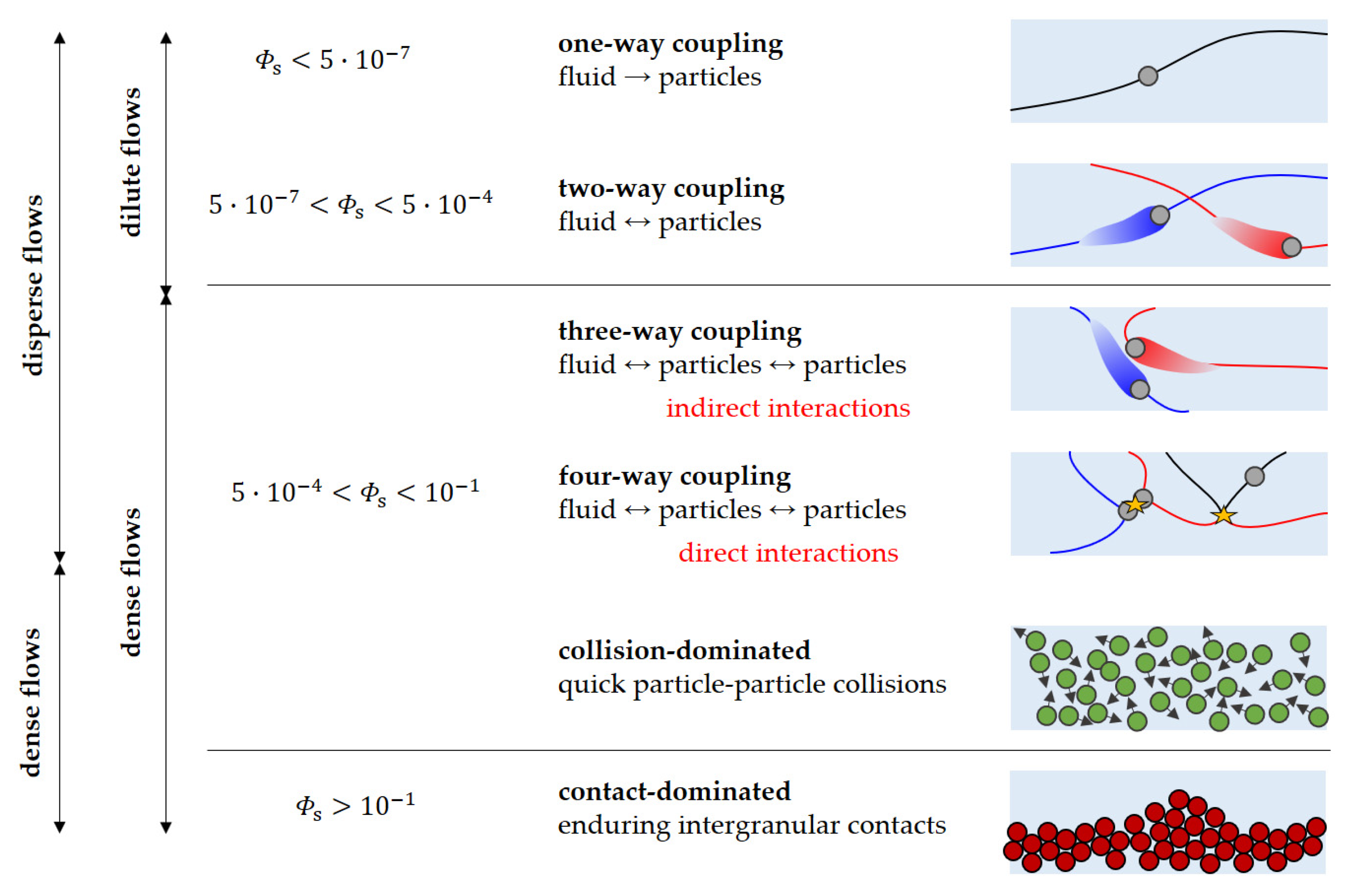
2. CFD Modelling Approaches

The modelling approaches for the CFD simulation of slurry flows, already introduced in the previous section, will be now discussed. Particular attention will be paid to explaining the mathematical basis of each approach, including the fundamental governing equations, the additional equations needed (constitutive equations and other closures), and the modelling of turbulence, and the typical boundary conditions employed in slurry pipe problems. Although the authors’ intention is to provide a comprehensive overview of the modelling approaches, underlining which are their assumptions and how they are related to each other, it was not possible to present all the mathematical details, nor all the possible available options for the constitutive equations and closures. For further information, the reader is referred to the several papers/textbooks/reports specifically dedicated to the topic, including, among others [32,33,34,35,39].

2.1. Eulerian–Lagrangian Modelling

In the Eulerian–Lagrangian (EL) approach, the carrier liquid is modeled as a continuum, and therefore normally referred to as the continuous phase in a multiphase flow simulation. For an isothermal flow, the mass and linear momentum equations must in general be solved:
ρ l t + · ρ l u = 0
ρ l u t + · ρ l u u = · σ l + ρ l g
where ρ l is the density of the liquid, u is the instantaneous velocity vector of the liquid, and g is the gravitational acceleration vector. Normally, in an isothermal flow, the density of a liquid can be regarded as a constant under moderate pressures. In such situations, the equations above can be further simplified:
· u = 0
ρ l ( u t + · u u ) = · σ l + ρ l g
In Equations (2) and (4) above, σ l denotes the stress tensor of the liquid phase, which depends on the fluid rheology. The typical approach is to split σ l into the sum of an isotropic part, p l I (where p l is the pressure of the liquid phase), and a deviatoric part, referred to as τ l . The main interest in this article is on Newtonian carrier fluids, for which, in the case of incompressible flow, the expression below holds:
σ l = p l I + τ l = p l I + μ l [ u + ( u ) + ]
where μ l is the dynamic viscosity of the liquid phase, and the superscript “+” indicates that the transpose of the dyadic u is taken.
The equations illustrated so far are intended to be the instantaneous ones, valid for both laminar and turbulent flows. Depending on the Reynolds number, the non-linear term on the LHS of Equation (4) can give rise to a huge number of degrees of freedom, i.e., the flow becomes turbulent. In order to keep the computational burden within acceptable limits and meet the engineering needs, the modelling of turbulent flows is generally carried out by solving only for the mean flow or the largest scales of turbulence. Solving for all the time and space scales that arise in a turbulent flow may be unaffordable in most practical situations, or not even convenient. A usual approach is then to apply a Reynolds average. Mathematically, it consists in applying the time average to all variables, that is,
ψ ¯ ( r , t ) = t T 2 t + T 2 ψ ( r , τ ) d τ
where ψ is the generic volume-averaged variable, and T is a time scale much larger than those of the turbulent fluctuations and much smaller than the time scale of the macroscopic flow. The trace denotes an average in time. By applying this operation to Equations (3) and (4), we obtain:
· u ¯ = 0
ρ l ( u ¯ t + · u ¯ u ¯ ) = · σ ¯ l + ρ l g · ρ l u u ¯
For the sake of simplicity, from this point onwards, the equations above will be written as:
· U = 0
ρ l ( U t + · U U ) = · σ ¯ l + ρ l g · ρ l u u ¯
where u is the fluctuation velocity, whereas U = u ¯ is the average velocity. By summing both, the instantaneous fluid velocity u is obtained. The last term in Equation (10) is the Reynolds stress tensor. This term must be modeled so that the set of equations has a solution. Within the Reynolds-average approach (RANS), there are essentially two options: use the Boussinesq hypothesis, which assumes that the turbulent fluid motion is analogous to the molecular motion, so that an eddy viscosity concept is proposed; or solve for all the Reynolds stress components. In the latter, by virtue of symmetry of the shear stress tensor, six additional transport equations must be solved, by the differential Reynolds Stress Model (RSM), or six additional algebraic closures must be used, with the algebraic Reynolds Stress Model. According to the Boussinesq approach, for incompressible flows
ρ l u u ¯ = μ l t ( U + ( U ) + ) 2 3 ρ l k l I
where μ l t is the eddy viscosity of the liquid, and k l is the turbulent kinetic energy per unit mass of the liquid. Thus, for incompressible RANS models based on the Boussinesq approach, the final set of equations for the fluid can be written as:
· U = 0
ρ l ( U t + · U U ) = P l + · [ μ l eff ( U + ( U ) + ) ] + ρ l g
where μ l eff represents the effective viscosity of the liquid, and it is calculated as the sum of the molecular viscosity μ l and the eddy viscosity μ l t , and P l is equal to the time-averaged pressure p l plus 2 / 3 ρ l k l . There are a number of models for computing the turbulence viscosity, such as k -𝜀, SST k - ω , and Spalart–Allmaras. As it is not the purpose of this article to discuss these models, the reader is referred to Menter [40], Launder and Spalding [41] for further information and theoretical background. Equations (12) and (13) or (10), along with the turbulence model equations, form the basis for the Eulerian fashion as applied to the liquid.
Generally, the fluid flow equations discussed here above are numerically solved using grid-based methods such as the Finite Volume Method, the Finite Difference Method, or the Lattice–Boltzmann Method [42]. Depending on the ratio of mesh size to particle diameter, Eulerian–Lagrangian models can be classified into point-particle (or unresolved) methods and fully-resolved methods. If the particle dimensions are negligible as compared to the fluid cell, then the point-particle approximation can be made, which consists in assuming that the particles are point sources of momentum with zero dimension (Figure 6a). At the opposite extreme, fully-resolved methods require the grid size to be much smaller than the particle size and model accurately the flow around the solid particle (Figure 6b). Such point-particle approximation is generally made in Euler–Lagrange simulations for engineering purposes, although a fully-resolved treatment is feasible with supercomputing resources.
In both approaches, the equation of motion for each particle is based on Newton’s second law. Each particle is tracked individually throughout the fluid domain. In particular, it is important to solve for the angular momentum in pipe flows, because collisions with walls are frequent. The trajectory, linear momentum and angular momentum conservation equations for a rigid, constant-mass particle can be written as:
d r p d t = v p
m p d v p d t = F p
I p d ω p d t = T p
where r p , v p , and ω p are the position vector, the velocity vector, and the angular velocity vector of the particle, respectively, m p is the mass of the particle, I p is the moment of inertia of the particle, and F p and T p are the forces and the torque exerted on the particle, respectively.
As can be observed, the motion equations for the Lagrangian approach are much simpler than those for the Eulerian one. Essentially, only ordinary differential equations are involved, unlike the partial differential equations necessary to describe the fluid. The external forces acting on a particle, F p , may be due to force fields, fluid–particle interaction and particle–particle interaction. There are basically two classes of forces that a particle can experience: body (or field) forces, and surface forces. As body forces, the most important ones are weight and buoyancy. Surface forces obviously require contact between the particle and the agent causing the force, which can be either the fluid, another particle, or a solid wall. Regarding external torques on a particle, T p , the main driving mechanisms are the contact with the fluid, interparticle collisions and particle-to-wall collisions.
The evaluation of the fluid–particle forces and torques is carried out differently in fully resolved and point-particle models. Since, in fully-resolved models, the mesh resolution is much smaller compared to the particle size, the action from the fluid to a particle can be directly obtained by integrating the pressure and viscous stresses distributions over the particle surface (Figure 6b). Conversely, in point-particle models, the forces and torques on the RHS of Equations (15) and (16) cannot be computed directly. Thus, correlations for the external forces and torques acting on each particle must be obtained from appropriate force models, devised either from experiments or from surface-resolved Direct Numerical Simulations.
Models for liquid-to-particles surface forces include, among others, drag, shear-induced lift, pressure gradient and virtual mass. The drag force is often the dominant one in liquid–solid flows, and it is calculated as:
F d = 1 2 ρ l ( π d p 2 4 ) C d | u @ p v p | ( u @ p v p )
where d p is the equivalent diameter of a particle (that is, the diameter of the volume-equivalent sphere), C d is the drag coefficient, and u @ p is the fluid velocity at the particle position, called unhindered fluid velocity. The drag coefficient can be obtained as a function of the particle Reynolds number based on the particle diameter:
R e p = ρ l d p | u @ p v p |   μ l
and possibly additional parameters. As will be further discussed in Section 3, several correlations exist for the evaluation of the drag coefficient, which have different applicability limits in terms of range of R e p values, shape of particles, etc. Very often, the user of a CFD code has no basis to select one formula instead of another, but this choice might have an impact on the numerical solution. This is even more true for the values of particle shape-related coefficients which appear in the drag coefficient correlations for non-spherical particles, as these coefficients are likely to play a significant role in liquid–solid flows, but are very difficult to decide. Therefore, the formula for the drag coefficient and the value of its coefficients are important sources of uncertainty for the CFD results.
As shown in Equations (17) and (18) above, many force models depend on flow features at the particle position. At this point, it should be noted that, because RANS models are designed to yield a mean fluid velocity field only, the fluid velocity at the cell centers do not contain the fluctuating component typical of a turbulent flow. At a given point in space, it essentially remains the same in time, which is not consistent with the nature of turbulent flow. The point here is that particles are sensitive to the instantaneous flow, not just the mean flow. It is thus necessary to add a fluctuating velocity component to the average fluid velocity at the particle position U @ p . This fluctuating velocity is not simply a randomly sampled number; it must reflect the local turbulence properties. This can be accomplished by a turbulence dispersion model, such as those proposed by Gosman and Ioannides [43] and Sommerfeld et al. [44].
An important aspect of the Euler–Lagrange approach based on the point-particle approximation is related to the number of particles to be used in a simulation. Ideally, all the particles in a physical system should be simulated, however even dilute flows may contain billions of particles depending on the pipeline dimensions. Despite the tremendous advances in hardware over recent decades, simulating every single physical particle is not practical, and especially in the context of RANS, unnecessary. Instead, computational particles, also named parcels, are used. The basic concept is that a parcel represents a number of physical particles with the same velocity and diameter, at the same position. This substantially saves computer time, while not hindering particle statistics, as the main interest in RANS simulations lies in average properties. In the remainder of this paper, the subscript “P” will be used to denote a parcel, whereas “p” indicates a physical particle.
As discussed, point-particle methods and fully-resolved methods impose strict constraints on the size of the grid used for fluid flow calculation, which must be much larger and much smaller compared to the particle diameter, respectively. In order to translate this concept into practical recommendations, threshold values must be given for the ratio of mesh size to particle diameter. It was reported [45] that, in fully-resolved methods, the mesh size should be at most 1/8 of the particle diameter so that numerical errors can be limited. Increasing the ratio of mesh size to particle diameter, e.g., bigger than 1/5, can lead to rough representation of particle boundary and thus inaccurate results. To avoid an undesirable increase in computing power when using a fine mesh throughout the whole computing area, it is possible to use the local dynamic mesh refinement close to the particle surface [45]. However, still, the fully-resolved method is suitable only for processes where the number of particles is limited (in the order of hundreds or thousands). As an example of the largest systems studied with this approach, in [46] simulations of river bed forms was carried out on 24,756 cores, and only 350,000 particles were tracked, which is much less than the point-particle methods, where the number of particles can reach tens of millions. At the opposite extreme, the literature showed that not only the basic idea underlining point-particle models, but also the accuracy of widely used force models is affected by the grid size. Peng et al. [47] recommended that, in order to ensure the accurate calculation of the relative velocity and the void fraction in different drag force models, the mesh size should be at least three times larger than the particle diameter. Otherwise, by reducing the ratio of mesh size to particle diameter to smaller than 3, the drag force model can be inaccurate with a large deviation from experimental results. Apparently, for the EL modeling of particulate flows, there exists a grey zone, as, if the ratio of mesh size to particle diameter ranges from 1/8 to 3, both point-particle and fully-resolved modeling are not accurate. There is a clear gap for the situations with a size ratio ranging from 1/8 to 3. In order to bridge it, several approaches have been proposed, such as the statistical kernel method, the porous cube method, the big sphere method and the diffusion approach [48].

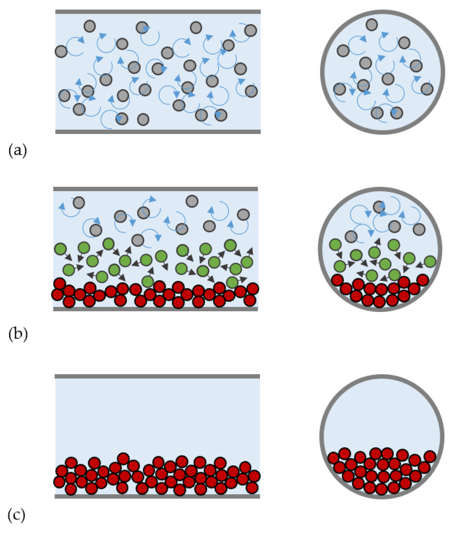
2.1.1. One-Way Coupled Slurry Flows

Equations (12)–(16) form the basis of the Eulerian–Lagrangian approach. Particles are directly affected by the fluid flow, since the forces and torques are partly caused by the fluid. However, this set of equations, as they are herein presented, do not account for the effect of the particles on the fluid flow. This is the one-way coupling regime, which, as already discussed in Section 1.3, is valid only in flows with a low particle concentration (Figure 3). Depending on the local particle concentration, the impact of the particles on the fluid cannot be disregarded. In such cases, the reaction of the particles to the fluid must be taken into account. Additionally, interparticle collisions may play a role. These will be dealt with in the following sections.

2.1.2. Two and Four-Way Coupled Slurry Flows

In the two-way coupling regime, and under the point-particle approximation, the momentum exchanged between the particle and the fluid must be added to the RHS of Equation (13):
S l = 1 W m P [ d v P d t ( 1 ρ p ρ l ) g ]  
where the summation applies to all parcels contained in volume W . In compliance with Newton’s Third Law, body forces should not be considered. In Equation (19), it is assumed that only body forces experienced by the particles are weight and buoyancy. Another peculiar feature of two-way coupled Eulerian–Lagrangian models resides in the presence, in the equations of the turbulence model, of source terms associated with the influence of the particles on the turbulence characteristics of the carrier fluid. This phenomenon is called turbulence modulation, and it is characteristic of the two-way coupling regime; particularly, the evidence shows that fine particles tend to attenuate the turbulence in the carrier fluid phase, whereas turbulence enhancement occurs in the case of coarse solids [29]. The modelling methods to account for this effect will be discussed more deeply in Section 2.2.4.
Particle-to-particle collisions may become important at higher concentrations. Even under “disperse” operating conditions, in the sense given by Loth [28] (Figure 3), interparticle collisions may be important in redispersing particles in pipe flows, acting as a diffusion mechanism, especially in locally concentrated regions. If they are to be considered, we then have the so-called four-way coupling. There are different possibilities for modeling such forces: hard-sphere and soft-sphere models exist. In the latter, the mechanical properties of the particle material must be used to calculate the tiny deformation that occurs during a collision, while the former assumes that particles are perfectly rigid. The Discrete Element Method (DEM) commonly employs a soft-sphere model, using one of the several models available for normal contact forces, namely linear spring–dashpot, and non-linear damped Hertzian spring–dashpot, among others. The soft sphere model requires determining the normal spring stiffness coefficient of the linear model through the numerical solution for the overlap between particles in non-linear models. Irrespective of the interparticle collision model, a coarse-graining procedure is needed in accordance with the parcel concept, except for very dilute systems for which every single particle can be represented.
Although both models discussed above are perfectly applicable to densely concentrated slurries, the issue of computational cost may turn the simulations unfeasible. For smooth statistics, a huge number of parcels might be necessary. In such situations, there exist computationally cheaper options for considering interparticle collisions such as the Dense Discrete Particle Model (DDPM). In the DDPM, particle-to-particle collisions are accounted for by a collision force based on the distribution of the solid volume fraction and the granular temperature, by partially relying on the Kinetic Theory for Granular Flows (KTGF), whose fundamental formulation will be presented in the following sections.

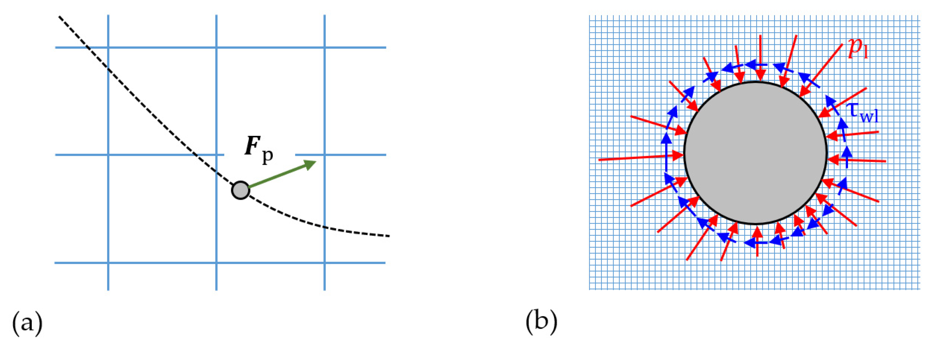
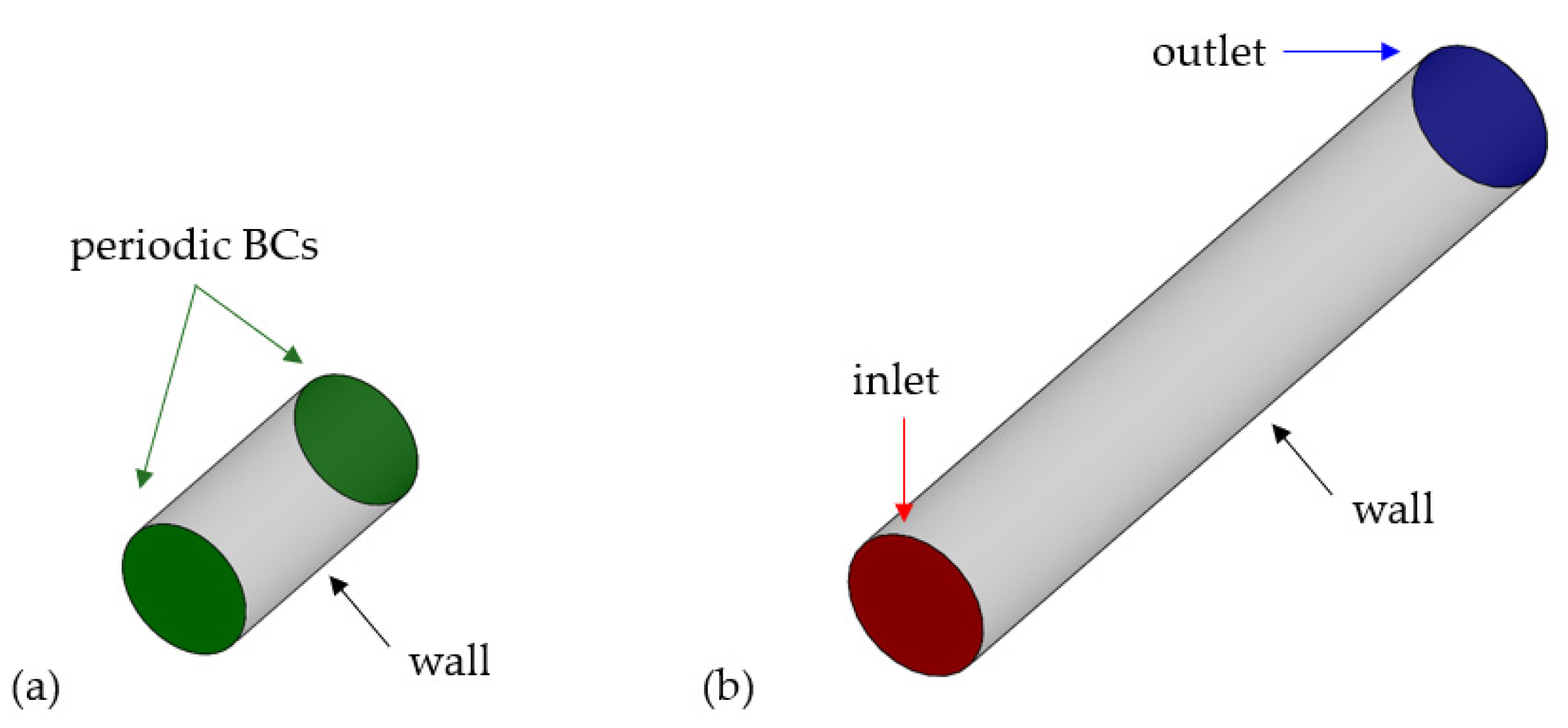
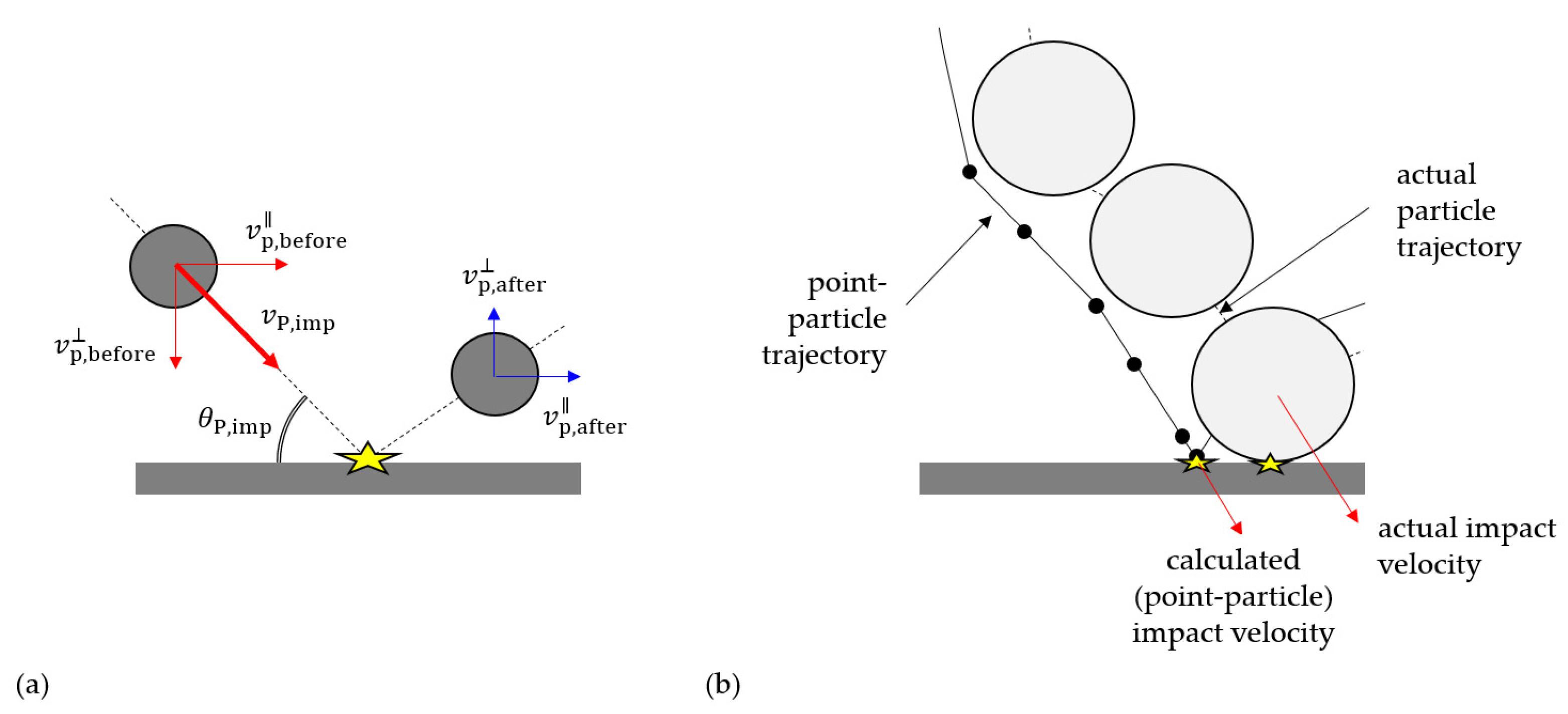
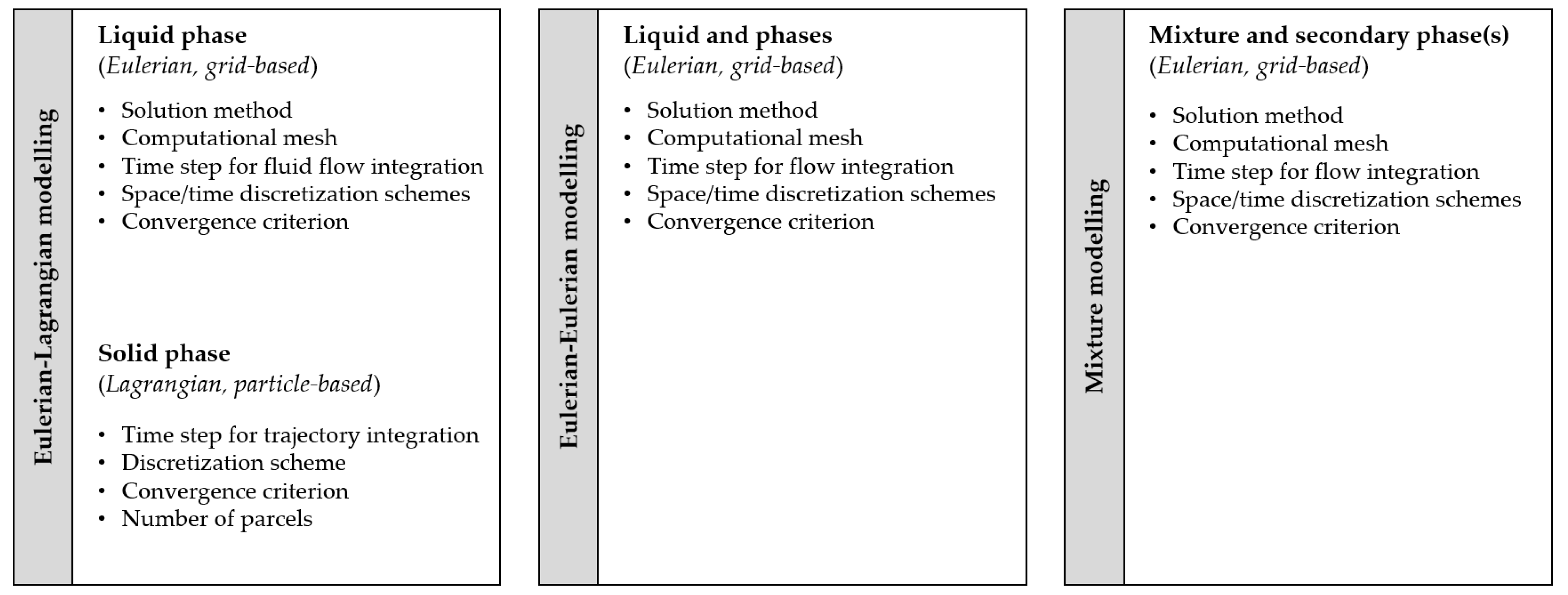
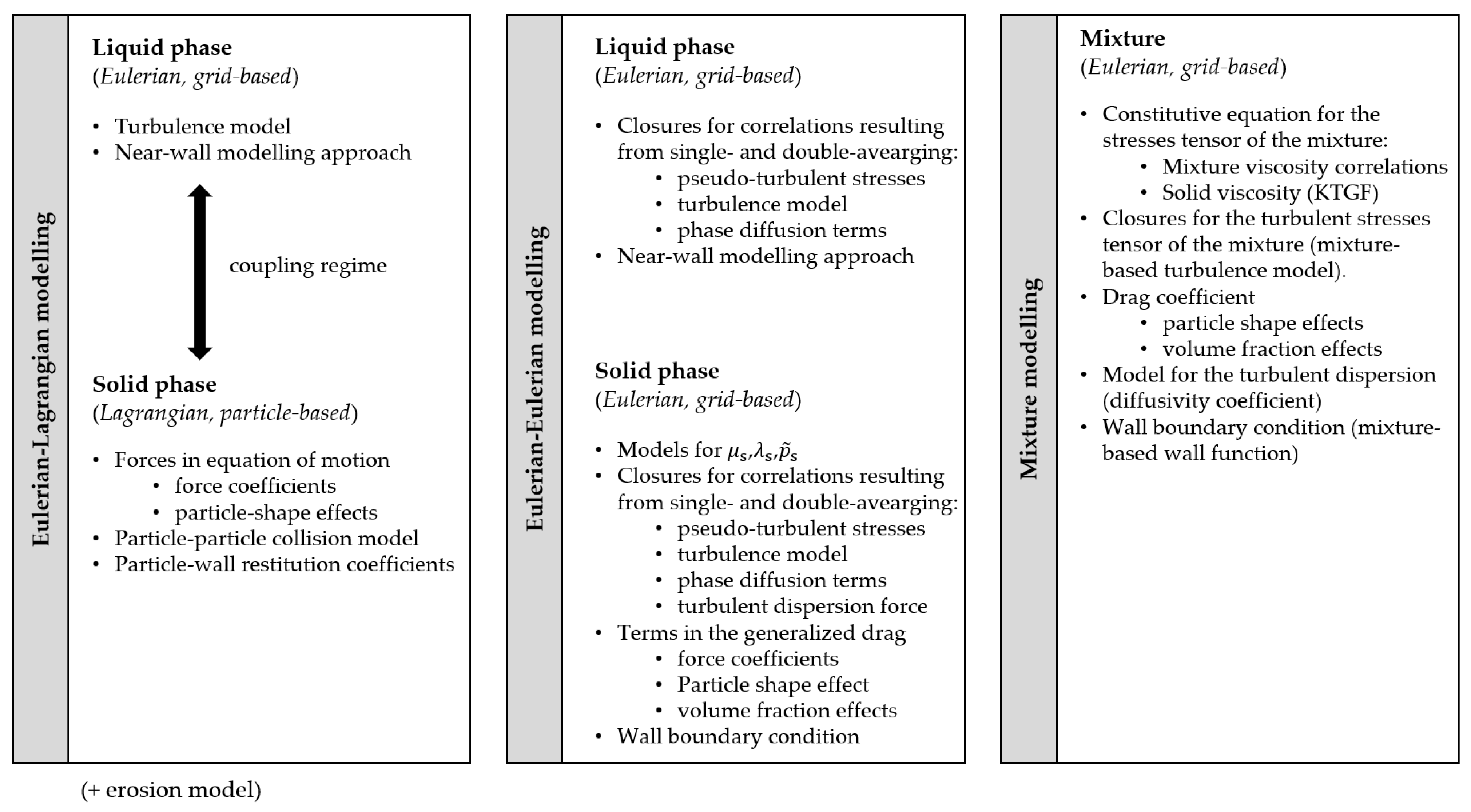
2.1.3. Boundary Conditions

Regarding boundary conditions for slurry flows in pipes, normally when the interest is in the fully developed flow, periodic conditions are applied to a pipe length (Figure 7a). A pressure drop or source term forcing a given mass flow must be prescribed as the driving force. Otherwise, classical inlet and outlet boundaries are used, i.e., the convective flux of the liquid, along with the turbulence quantities, are prescribed at the inlet boundary, whereas at the outlet the static pressure is specified and the normal gradient is zero for all liquid variables (Figure 7b). As for the particles, they are normally injected at the inlet with a given velocity, and are allowed to escape the outlet. It is worth noting that the applied boundary conditions scheme affects the length of pipe to be simulated to achieve fully developed flow. In fact, whereas a short pipe length is sufficient in the case of periodic boundary conditions, the domain must be longer if inlet–outlet conditions are used, since the flow must develop from the state imposed at the inlet boundary. Assessing the length of the pipe to be simulated is a significant feature of slurry pipe flow simulations, and it will be the subject of discussion in Section 3.1.
In both schemes, the pipe walls are treated as solid wall boundaries. No-slip conditions are adopted whenever the mesh resolution is enough to calculate the boundary layer profile. Alternatively, if not enough refinement is possible, the wall shear stress according to a given law-of-the-wall, such as Launder and Spalding’s [49], and different types of constraints on the turbulent variables are applied. As with other wall-bounded flows, the wall boundary conditions play an important role in pipe flows. This is because upon colliding with a wall, the particle exchanges linear and angular momentum. This may translate into an increase in the flow pressure drop, especially for horizontal flows, and more so for rough pipes. After a collision, the particle must be reaccelerated by the fluid. In order to maintain the mean fluid velocity, this reacceleration comes at the expense of increased inlet pressure. As demonstrated by Huber and Sommerfeld [50], wall roughness can play a very important role in horizontal pipe flows.
Wall–particle collisions are typically modeled by imposing normal and tangential restitution coefficients, e n and e t , which relate the normal and tangential components of parcel velocity after and before the impact against the wall, that is,
e n = v p , after v p , before e t = v p , after v p , before
where all symbols are indicated in Figure 8a. These coefficients are usually expressed as a function of the particle (or parcel-) wall impact angle, θ p , imp , by means of empirical correlations. The collisions can be sliding or non-sliding, depending on the coefficients of restitution and friction, as discussed by Breuer et al. [51]. In general terms, the correlation employed for evaluating e n and e t might have an effect on the solution of an Eulerian–Lagrangian model, and this modelling feature might act as a significant source of uncertainty in slurry erosion prediction simulations (see Section 3.2.1). An important feature that deserves some attention is that, although the derivation in [51] accounts for the particle finite radius during collisions, most implementations of the Euler–Lagrange approach are performed under the point-particle approximation and they estimate the collision as if occurring at the wall (Figure 8b). This may result in inaccuracy, mainly in erosion predictions, as demonstrated by Messa and Wang [52]. This topic will be further discussed in Section 4.3.2.

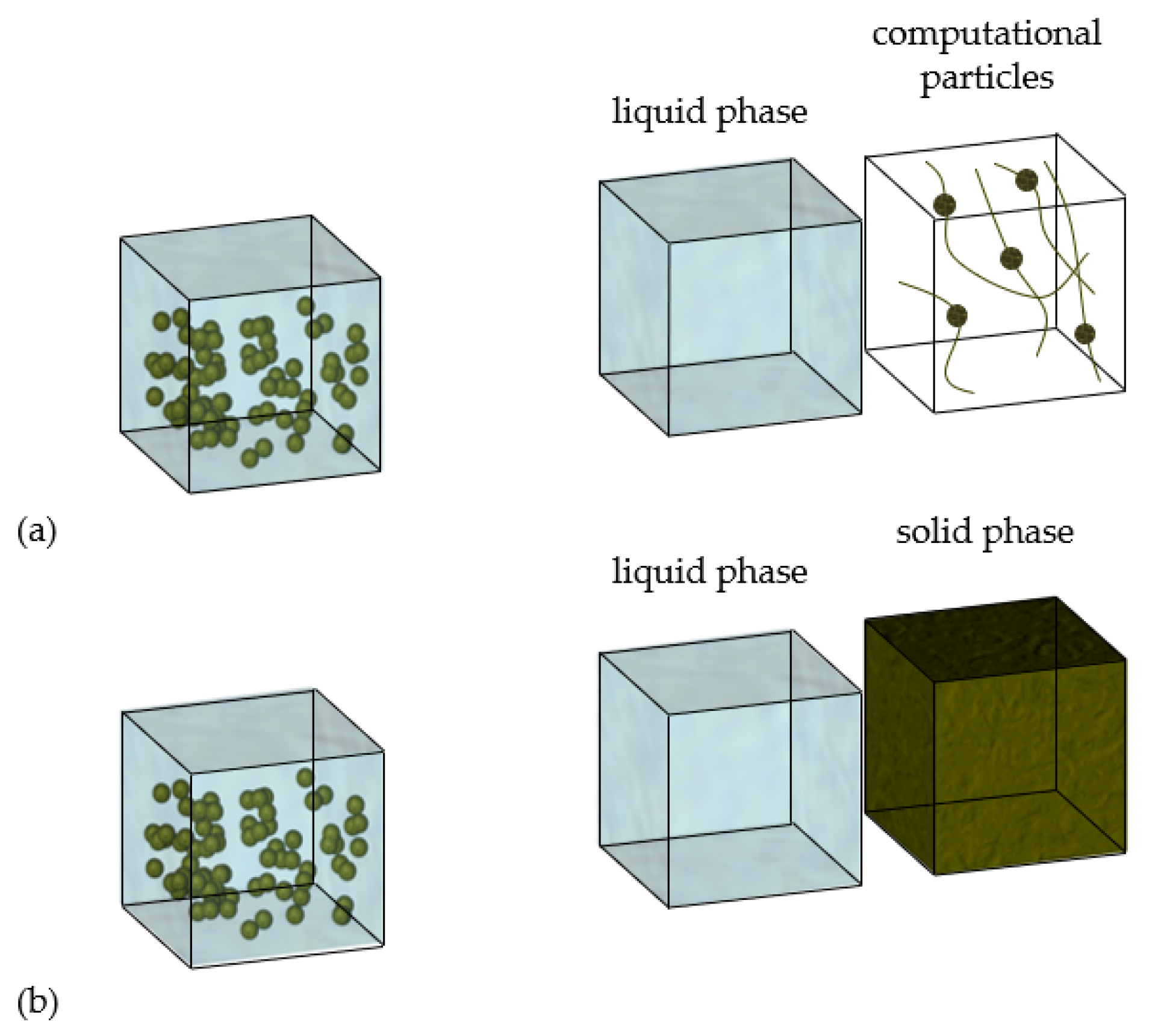
2.2. Eulerian–Eulerian Modelling (Two-Fluid Modelling)

2.2.1. Fundamental Conservation Equations

In the Eulerian–Eulerian approach, both phases are interpreted as interpenetrating continua and they are modeled in the Eulerian, cell-based framework. This is achieved by solving for the fundamental mass and momentum conservation equations for two media, namely, the carrier liquid and a fictitious fluid representing the fluid dynamic behavior of the ensemble of solid particles, called “solid phase”. The instantaneous equations of the two-fluid model can be derived in different ways, and they typically read as follows:
ϕ ˜ l ρ l t + · ϕ ˜ l ρ l u ˜ = 0
ϕ ˜ s ρ s t + · ϕ ˜ s ρ s v ˜ = 0
ϕ ˜ l ρ l u ˜ t + · ϕ ˜ l ρ l u ˜ u ˜ = · ( ϕ ˜ l σ ˜ l ) + ϕ ˜ l ρ l g + m ˜ l + · σ pt , l  
ϕ ˜ s ρ s v ˜ t + · ϕ ˜ s ρ s v ˜ v ˜ = · ( ϕ ˜ s σ ˜ s ) + ϕ ˜ s ρ s g + m ˜ s + · σ pt , s
The above equations are the mass and momentum conservation of the liquid and the solid phases, respectively. Probably the most intuitive approach in the Eulerian–Eulerian framework consists in referring to a sampling volume W , centered in each space point r and large enough to obtain reliable statistics for the two-phase mixture (Figure 9). In this study, the fluid dynamic parameters referred to as the sampling volume are denoted by a tilde. Particularly, ϕ ˜ l ( r , t ) and ϕ ˜ s ( r , t ) can be interpreted as the fraction of the sampling volume centered in r , which at time t , is occupied by one phase. The velocity vectors,   u ˜ and v ˜ , and the stresses tensors, σ ˜ l and σ ˜ s , are defined as the average over the amount of phase in W . Conversely, the terms m ˜ l and m ˜ s represent the total force exerted on the current phase by the other one in the sampling volume, divided by the sampling volume itself.
The volume-averaged Eulerian–Eulerian mass and momentum conservation equations show some formal similarity with the corresponding equations for a single-phase flow. Apart from the different meaning of the fluid dynamic variables (as indicated by the tilde), as well as the presence of the volume fractions, ϕ ˜ l ( r , t ) and ϕ ˜ s ( r , t ) , and of the momentum exchange terms, m ˜ l and m ˜ s , an important difference is represented by the terms · σ pt , l and · σ pt , s , which come up as a result of the volume-averaging of the convective accelerations. Tensors σ pt , l and σ pt , s are called pseudo-turbulent stress tensors to underline that, despite their evident analogy with the Reynolds-stresses tensor in the RANS equations for single-phase flows, in the case of particle-laden flows they can be nonzero even in the laminar regime.
Unlike Eulerian–Lagrangian models, Eulerian–Eulerian models are inherently two way coupled. Particularly, two types of coupling exist, namely, mass coupling and momentum coupling. The mass coupling is related to the fulfillment of the mass conservation equation of the mixture, which imposes that ϕ ˜ l + ϕ ˜ s = 1 . The momentum coupling relates with the action reaction principle, that is, m ˜ s = m ˜ l . Even if, in principle, a simplified formulation of Equations (21)–(24) could be derived for the specific case of one-way coupled particle-laden flows, to the best of the authors’ knowledge, this has never been attempted so far. Conversely, the two-fluid model is frequently applied to four-way coupled flows, in which inter-particle collisions and contacts are important. In the Eulerian–Eulerian framework, four-way coupling effects are accounted for through the constitutive equations for the pressure and the deviatoric stress tensor of the solid phase, as it will be discussed hereafter.

2.2.2. Constitutive Equations

Equations (23) and (24) must be solved in conjunction with constitutive equations for the stresses tensors of the two phases, σ ˜ k   ( k = l,s), and the typical approach is, once again, to split the two tensors into their isotropic and deviatoric parts, that is
σ ˜ k = p ˜ k I + τ ˜ k  
The modelling of the deviatoric stress tensor of the liquid phase is rather straightforward, since the volume-averaged analogues of the classical stress–strain relations of single-phase fluid dynamics are employed. For instance, a typical constitutive equation used for Newtonian carriers is:
σ ˜ l = p ˜ l I + τ ˜ l = p ˜ l I + μ l [ u ˜ + ( u ˜ ) + ] + ( λ l 2 3 μ l ) ( · u ˜ ) I  
where λ l is called the second viscosity coefficient. Note that, in principle, the volume-averaged velocity field u ˜ is not divergence-free for incompressible carriers. Therefore, the last term in Equation (26) is not identically zero, even if it is usually neglected in Euler–Euler models, obtaining a formally similar relation as in the classical Eulerian–Lagrangian approach (Equation (5)). However, the situation becomes more complicated for the solid phase. Solving Equation (25), in fact, requires facing the non-trivial challenge of how to characterize from a physical point of view (first) and how to evaluate (afterwards) the pressure and deviatoric stress tensor of the solid phase. Generally, a solid-phase analogous of Equation (26) is employed, as follows:
σ ˜ s = p ˜ s I + τ ˜ s = p ˜ s I + μ s [ v ˜ + ( v ˜ ) + ] + ( λ s 2 3 μ s ) ( · v ˜ ) I  
The first viscosity coefficient, μ s , is commonly associated with a kinetic effect, due to the free particle movement, a collisional effect, due to the particle–particle collisions, and a frictional effect, when the solid volume fraction approaches the packing value and particle interactions are reduced to frictional contacts. These effects are modeled separately, by expressing μ s as the sum of a kinetic viscosity, μ s , kin , a collisional viscosity, μ s , coll , and a frictional viscosity, μ s , fr , that is:
μ s = μ s , kin + μ s , coll + μ s , fr  
The second viscosity coefficient, λ s , also called bulk viscosity of the solid phase, describes the resistance of the agglomeration of particles against expansion and compression. As far as the pressure of the solid phase is concerned, the typical approach is to split the product ϕ ˜ s p ˜ s into three terms, as follows
ϕ ˜ s p ˜ s = ϕ ˜ s p ˜ l + p ˜ s , kin + p ˜ s , coll  
where the sum of the kinetic component, p ˜ s , kin , and of the collisional component, p ˜ s , coll , is sometimes referred to as solid pressure. As their names themselves say, p ˜ s , kin and p ˜ s , coll are associated to the already mentioned kinetic and collisional effects, whilst ϕ ˜ s p ˜ l accounts for a sort of “buoyant” effect, that is, a fluid pressure gradient through a collective of solids will exert a force on the particles, changing the particle pressure [39].
In most studies concerning the Eulerian–Eulerian modelling of slurry flows in pipes, the constitutive parameters μ s , kin , μ s , coll , μ s , fr , λ s , p ˜ s , kin , and p ˜ s , coll were obtained from the Kinetic Theory of Granular Flow (KTGF), based on the kinetic theory of gases where a granular temperature, Θ s , is defined starting from the mean square of the solids velocity fluctuations, such that
Θ s = 1 3 v ˜ v ˜ ¯  
As it will be further discussed in Section 4.3.2, in the KTGF, the six variables listed above are algebraic functions of Θ s as well as other particle-related parameters, such as the restitution coefficient of particle–particle collisions, the solid volume fraction at maximum packing, and the angle of internal friction. The granular temperature, in turn, is obtained from the solution of its own transport equation. However, other two-fluid models for slurry pipe flow simulation do not rely on the KTGF but use empirical constitutive equations for μ s and p ˜ s . As far as μ s is concerned, a possible approach was mentioned in [39], which consists in estimating μ s from the viscosity of the mixture μ m
μ m = μ s ϕ ˜ s + μ l ϕ ˜ l  
which, in turn, can be evaluated as a function of ϕ ˜ s through the many empirical correlations reported in the literature [39,53] in a more or less rigorous way. On some occasions, p ˜ s was modeled as p ˜ l plus some empirical functions of the gradient of ϕ ˜ s , initially developed for fluidized bed reactors and representing the effect of particle–particle collisions [39,54]. Examples of two-fluid models based on the KTGF and on empirical constitutive equations for the solid phase will be presented in Section 4.3 and Section 4.4, respectively.

2.2.3. Interfacial Momentum Transfer

The terms m ˜ k   ( k = l,s), called interfacial momentum transfer terms, account for the exchange of forces between the two phases through their interface. Following Enwald et al. [39], these parameters can be expressed in terms of the interfacially-averaged pressure and deviatoric stress tensor, p ˜ i and τ ˜ i , as follows:
m ˜ k = m ˜ k d + p ˜ i ϕ ˜ k τ ˜ i · ϕ ˜ k  
where m ˜ k d is referred to as generalized drag, and it is the same as m ˜ k but evaluated in terms of the differences p ˜ k p ˜ i and τ ˜ k τ ˜ i . On the grounds of Equations (25) and (32), the RHS of Equations (23) and (24) become:
( ϕ ˜ k p ˜ k ) + · ( ϕ ˜ k τ ˜ k ) + ϕ ˜ k ρ k g + m ˜ k d + p ˜ i ϕ ˜ k τ ˜ i · ϕ ˜ k + · σ pt , k  
After some mathematical manipulation and taking into account the different contributions of the solid pressure, Equation (33) can be rewritten as:
ϕ ˜ k p ˜ l ( p ˜ s , kin + p ˜ s , coll ) only   if   k = s + · ( ϕ ˜ k τ ˜ k ) + + ϕ ˜ k ρ k g + m ˜ k d + ( p ˜ i p ˜ l ) ϕ ˜ k τ ˜ i · ϕ ˜ k + · σ pt , k  
where, clearly, the second term is present only in the momentum equation of the solid phase. The last two terms in Equation (34) are generally ignored in the two-fluid models used for simulating the type of flow considered in this review, as well as the pseudo-turbulent stresses tensor term, · σ pt , k . Therefore, the typical formulation of the momentum equations of Eulerian–Eulerian models is:
ϕ ˜ l ρ l u ˜ t + · ϕ ˜ l ρ l u ˜ u ˜ = ϕ ˜ l p ˜ l + · ( ϕ ˜ l τ ˜ l ) + ϕ ˜ l ρ l g + m ˜ l d  
ϕ ˜ s ρ s v ˜ t + · ϕ ˜ s ρ s v ˜ v ˜ = ϕ ˜ s p ˜ l ( p ˜ s , kin + p ˜ s , coll ) + · ( ϕ ˜ s τ ˜ s ) + ϕ ˜ s ρ s g + m ˜ s d
Owing to already mentioned momentum mass and momentum coupling constraints, it immediately follows that m ˜ s d = m ˜ l d . The generalized drag force acting on a suspension of solid particles is typically evaluated by employing the surface force models already introduced in Section 2.1. The drag force is the dominant term in most slurry pipe flows; under the assumption of considering only this effect, m ˜ s d is calculated as:
m ˜ s d = m ˜ l d = N p f ˜ l s W = N p W [ 1 2 ρ l C ˜ d ( π d p 2 4 ) | u ˜ v ˜ | ( u ˜ v ˜ ) ]  
where N p is the number of particles in the volume W , and f ˜ l s is output of the drag force model evaluated with respect to the volume-averaged velocities u ˜ and v ˜ . Similarly, C ˜ d means that the single-particle drag coefficient correlations are employed with the particle Reynolds number evaluated in terms of | u ˜ v ˜ | . Considering that:
N p W = ϕ ˜ s 4 3 π ( d p 2 ) 3  
it is possible to rewrite Equation (37) as
m ˜ s d = m ˜ l d = 3 4 d p ϕ ˜ s ρ l C ˜ d | u ˜ v ˜ | ( u ˜ v ˜ )  
In addition to the drag force, f ˜ l s might include also other forces, such as shear lift force, rotational lift force, added mass force, etc. As for the drag force, these terms are usually calculated employing the same expressions of point-particle Eulerian–Lagrangian models, after replacing the parcel-related quantities with the volume-averaged ones. However, as will be discussed in Section 3.2.2, in order to account for the different fluid dynamic resistance encountered by a single particle in a liquid and by the same particle in a liquid–solid mixture, empirical corrections are applied to C ˜ d , or different correlations are employed.

2.2.4. Modelling of Turbulent Flows

The equations illustrated so far are intended to be the instantaneous ones, valid for both laminar and turbulent flows. However, to keep the computational burden within acceptable limits and meet the engineering needs, the modelling of turbulent flows is generally carried out by solving only for the mean flow or the largest scales of turbulence. However, the Eulerian–Eulerian analogous of the RANS approach for single-phase flow is definitely complex to derive, as well as to characterize and justify from a physical point of view. In this regard, the double-average approach provides a strong mathematical ground for the derivation of the two-fluid models for turbulent flows. Essentially, the idea is to start from the instantaneous, volume-averaged equations and apply a second averaging operator, obtaining double-averaged equations whose unknowns are the double-average of the fluid dynamic variables (pressure, velocity, volume fraction, etc.). For the second averaging operator, two main options have been documented in the literature. The former consists of applying the same time average operator in Equation (6) to all volume-averaged variables, that is,
ψ ˜ k ¯ ( r , t ) = t T 2 t + T 2 ψ ˜ k ( r , τ ) d τ  
The latter option is to use the time average for all variables except for the velocity, to which the Favre operator is applied
u ˜ ( r , t ) = ϕ ˜ l u ˜ ¯ ϕ ˜ l ¯   v ˜ ( r , t ) = ϕ ˜ s v ˜ ¯ ϕ ˜ s ¯  
As illustrated by Burns et al. [55], the fundamental conservation equations assume different forms according to the second averaging operator applied. This is immediately evident in the mass conservation equations. After time-averaging, the mass conservation equations become:
ϕ ˜ l ¯ ρ l t + · ϕ ˜ l ¯ ρ l u ˜ ¯ + · ρ l ϕ ˜ l u ˜ ¯ = 0
ϕ ˜ s ¯ ρ s t + · ϕ ˜ s ¯ ρ s v ˜ ¯ + · ρ s ϕ ˜ s v ˜ ¯ = 0  
where ϕ ˜ l , ϕ ˜ s , u ˜ , v ˜ stand for the fluctuating component, namely, the difference between the instantaneous variable and its time-averaged value. Conversely, if the second averaging operator for the velocity is the Favre one, the double-averaged mass conservation equations read as follows:
ϕ ˜ l ¯ ρ l t + · ϕ ˜ l ¯ ρ l u ˜ = 0
ϕ ˜ s ¯ ρ s t + · ϕ ˜ s ¯ ρ s v ˜ = 0  
Comparing the two sets of equations above indicates that, when time-averaging of the volume-averaged mass conservation equations is performed, two additional terms come up, associated with the double correlations between the fluctuating velocity vector and the fluctuating volume fraction. These terms require modelling, which is typically achieved through the gradient diffusion approximation, initially proposed by Spalding [56] based on an analogy between the turbulent dispersion of solid particles and the turbulent diffusion of a passive scalar:
ϕ ˜ l u ˜ ¯ = μ l t ρ l σ ϕ ˜ l ¯   ϕ ˜ s v ˜ ¯ = μ l t ρ l σ ϕ ˜ s ¯
where μ l t is the already introduced eddy viscosity of the liquid phase, and σ is a numerical coefficient referred to as turbulent Schmidt number for volume fractions. The terms resulting from the application of the divergence operator to Equation (46) are called phase diffusion terms, and they are a distinctive character of some two-fluid models for the simulation of turbulent slurry transport in pipes, such as the β - σ model proposed by Messa and Matoušek [57], which will be subject of discussion in Section 4.5.2. Note that phase diffusion terms are present in all conservation equations, and not only in the mass conservation ones.
Whatever the second averaging operator is, double averaging of the momentum conservation equations produces several terms depending on double and triple correlations between fluctuations, which need to be modeled by additional closures. Elghobashi and Abou-Arab [58] reported the equations obtained by time-averaging the volume-averaged equations, and the momentum ones consist of about 15 terms. Most of these terms are simply ignored in commonly used two-fluid models, either because they are small or difficult to estimate. One might think that ignoring some terms might deviate the numerical solution from the physical one. However, it should be borne in mind that closure correlations are never exact, but they rely on approximations and empiricism: therefore, there is no guarantee that adding more closures results in higher accuracy, unless there is no doubt that such closures are applicable to the specific case study under investigation.
Given that, the double correlations associated with the convection terms are usually taken into account in slurry flow simulations. In the case of time-averaging of all variables, they are as follows:
ϕ ˜ l u ˜ u ˜ ¯ = ϕ ˜ l ¯ u ˜ ¯ u ˜ ¯ + ϕ ˜ l ¯ · u ˜ u ˜ ¯ + ϕ ˜ l u ˜ ¯ · u ˜ ¯ + ϕ ˜ l u ˜ u ˜ ¯ ϕ ˜ l ¯ u ˜ ¯ u ˜ ¯ + ϕ ˜ l ¯ · u ˜ u ˜ ¯ + ϕ ˜ l u ˜ ¯ · u ˜ ¯
ϕ ˜ s v ˜ v ˜ ¯ = ϕ ˜ s ¯ v ˜ v ˜ ¯ + ϕ ˜ s ¯ · v ˜ v ˜ ¯ + ϕ ˜ s v ˜ ¯ · v ˜ ¯ + ϕ ˜ s v ˜ v ˜ ¯ ϕ ˜ s ¯ v ˜ v ˜ ¯ + ϕ ˜ s ¯ · v ˜ v ˜ ¯ + ϕ ˜ s v ˜ ¯ · v ˜ ¯
whilst, if the volume-average velocity is Favre-averaged, the form of the double-averaged convection terms is:
ϕ ˜ l u ˜ u ˜ ¯ = ϕ ˜ l ¯ u ˜ u ˜ + ϕ ˜ l u ˜ u ˜ ¯
ϕ ˜ s v ˜ v ˜ ¯ = ϕ ˜ s ¯ v ˜ v ˜ + ϕ ˜ s v ˜ v ˜ ¯
where u ˜ and v ˜ are the differences between the volume-averaged velocity vectors and the Favre averaged quantities, that is u ˜ = u ˜ u ˜ and v ˜ = v ˜ v ˜ . The three terms on the right-hand side of Equations (47) and (48) are as follows: the first ones, ϕ ˜ l ¯ u ˜ ¯ u ˜ ¯ and ϕ ˜ s ¯ v ˜ v ˜ ¯ , include only the primary unknowns of the CFD simulation; the second ones, ϕ ˜ l ¯ · u ˜ u ˜ ¯ and ϕ ˜ s ¯ · v ˜ v ˜ ¯ , involve double correlations between the fluctuating velocities; the third ones, ϕ ˜ l u ˜ ¯ · u ˜ ¯ and ϕ ˜ s v ˜ ¯ · v ˜ ¯ , involve double correlations between the fluctuating velocities and the fluctuating volume fractions. The correlations ϕ ˜ l u ˜ ¯ and ϕ ˜ s v ˜ ¯ can be modeled through the gradient diffusion approximation (Equation (46)), and this explains why phase diffusion terms are present also in the momentum conservation equations. Conversely, Equations (49) and (50) include only two terms, the former with the primary unknowns and the latter consisting of triple correlations.
The modelling of terms ϕ ˜ l ¯ · u ˜ u ˜ ¯ and ϕ ˜ l u ˜ u ˜ ¯ is typically made as for the Reynolds stresses in single-phase flows, that is, either by solving for transport equation for each of the six independent terms or by applying a Boussinesq-like approximation (Equation (11)), which generally has the same form for the two types of averaging operators:
ϕ ˜ l ¯ · u ˜ u ˜ ¯ ϕ ˜ l ¯ { μ l t ρ l [ u ˜ ¯ + ( u ˜ ¯ ) + ] 2 3 μ l t ρ l ( · u ˜ ¯ ) I 2 3 k l I }
ϕ ˜ l u ˜ u ˜ ¯ ϕ ˜ l ¯ { μ l t ρ l [ u ˜ + ( u ˜ ) + ] 2 3 μ l t ρ l ( · u ˜ ) I 2 3 k l I }
As in single-phase flows, the last terms of Equations (51) and (52) do not appear explicitly in the momentum equation of the liquid, as they are usually combined with the pressure gradient one (see Section 2.1). In such eddy viscosity based models, μ l t is obtained from two-phase analogous of the turbulence models for the single-phase case. A formulation of the two-phase k - ε turbulence model consistent with the time- and volume-averaged operators was derived by Elghobashi and Abou-Arab [58], in which the two equations for the turbulent kinetic energy and the turbulent dissipation rate consist of 38 and 67 terms, respectively. However, much simpler formulations are used in engineering computations. For instance, the two-phase k - ε turbulence model by Spalding [56] has been frequently used to simulate turbulent slurry flows in pipes, and it reads as follows:
ϕ ˜ l ¯ ρ l k l t + · ϕ ˜ l ¯ ρ l u ˜ ¯ k l = · [ ϕ ˜ l ¯ ( μ l + μ l t σ k l ) k l ] + ϕ ˜ l ¯ ρ l ( P k l ε l ) + · ( μ l t σ k l ϕ ˜ l ¯ )
ϕ ˜ l ¯ ρ l ε l t + · ϕ ˜ l ¯ ρ l u ˜ ¯ ε l = · [ ϕ ˜ l ¯ ( μ l + μ l t σ ε l ) ε l ] + ϕ ˜ l ¯ ρ l ε l k l ( C 1 ε l P k l C 2 ε l ε l ) + · ( μ l t σ ε l ϕ ˜ l ¯ )
μ l t = C μ l ρ l k l 2 ε l
where P k l is the volumetric production rate of k l
P k l = 2 μ l t ρ l · 1 2 [ u ˜ ¯ + ( u ˜ ¯ ) + ] : u ˜ ¯  
and the values of the numerical coefficients are the same as in single-phase flows, namely, σ k l = 1.0, σ ε l = 1.314, C 1 ε l = 1.44, C 2 ε l = 1.92, and C μ l = 0.09. Basically, all two-equation models applied to slurry pipe flows are variations to the formulation of Spalding [56]; for instance, some of them do not include the phase diffusion terms; others include some corrections to account for specific effects, for instance, a high streamline curvature; still, others refer to different turbulent variables, such as the specific dissipation rate ω l instead of the turbulent dissipation rate, ε l . However, their basic structure is substantially the same.
A peculiar feature of some two-phase, two-equation models is the introduction, in the transport equations of the turbulent parameters (e.g., k l and ε l ), of source terms that account for turbulence modulation. As already mentioned in Section 2.1.2, this phenomenon is the variation of the turbulence characteristics of the carrier fluid produced by the presence of the solid particles, and it is characteristics of particle-laden flows (mostly gas–solid, but also liquid–solid) in the two-way coupling regime. The origin of the additional sources in the turbulence model equations, which account for the turbulence modulation, has been explained by Crowe [59] by deriving the conservation equation for the turbulent kinetic energy of the carrier fluid from the momentum equation of the same phase. Finally, the source terms in the k l -equation turned out to be related with the generalized drag term, and they include double correlations between the fluctuating velocities of the two phases, e.g., u ˜ v ¯ , which need to be modeled. Most of the available options are empirical or semi-empirical formulas developed for gas–solid flows (e.g., [60,61]), even if attempts to obtain such correlations from the KTGF and apply them to gas–solid and liquid–solid flows have been reported [62,63,64].
Mandø et al. [65] identified the main criticism of turbulence modulation models in the fact that, according to their derivation, they can predict only either turbulence attenuation or turbulence enhancement, as typical of particle-laden flows with fine and coarse particles, respectively. In order to overcome such limitations, these authors proposed a comprehensive model which can predict both effects at the same time. Such model, employed for simulating gas–solid flows using the Eulerian–Lagrangian approach, which was later generalized and applied to the Eulerian–Eulerian modelling of slurry flows in vertical pipes by Messa and Malavasi [66]. However, a key issue is that all available correlations were developed for dilute flows in the two-way coupling regime, for which the solid content is much lower compared to the high concentrations encountered in hydro-transport applications. The effect of turbulence modulation on the behavior of dense slurry flows, and its modelling, is an open problem. Indeed, in some papers the same expressions of the source term derived for dilute flows have been applied to dense liquid–solid flows in pipes, using the KTGF and empirical formulas for evaluating the correlations between the fluctuating velocities (e.g., [67]); however, no discussion was provided around the validity of such approach, nor it was assessed the actual impact of these terms on the CFD solution.
The modelling of the terms ϕ ˜ s ¯ · v ˜ v ˜ ¯ and ϕ ˜ s v ˜ v ˜ ¯ , which appear in the momentum equation of the solid phase, is even more confused. Generally, two-fluid models for slurry pipe flows based on the KTGF do not include those terms. Others apply a solid phase analogue of Equations (51) and (52), thereby introducing an eddy viscosity of the solid phase, μ s t , which is generally expressed as a function of μ l t through empirical, algebraic formulas developed for dilute gas–solid flows, e.g., [60,68,69]. The introduction of a differential particle turbulence model, with transport equations for the turbulent kinetic energy of the solid phase, k s , and its dissipation rate, ε s , was explored, for instance, by Mashayek and Taulbee [70] for gas–solid flows. Nonetheless, to the best of the authors’ knowledge, such approach has not been used for predicting slurry flows.
A peculiar feature of double-averaged two-fluid models resides in the modelling of the generalized drag terms, m ˜ l d = m ˜ s d . If only the contribution of the drag force is considered, which, as already remarked, is usually the dominant interfacial force in most slurry pipe flows, then m ˜ l d takes the form of Equation (39), but it is convenient to rewrite the formula as
m ˜ l d = C ls ( v ˜ u ˜ ) = D ls ϕ ˜ s ( u ˜ v ˜ )  
where
C ls = D ls ϕ ˜ s = 3 4 d p ϕ ˜ s ρ l C ˜ d | u ˜ v ˜ |  
According to Burns et al. [55], a reasonable first approximation is to treat D ls as constant during the averaging process. Under this assumption, time-averaging of Equation (57) yields:
m ˜ ¯ l d D ls ϕ ˜ s ¯ ( v ˜ ¯ u ˜ ¯ ) + D ls ϕ ˜ s ( v ˜ u ˜ ) ¯  
Considering that ϕ ˜ l ¯ + ϕ ˜ s ¯ = 1 and that ϕ ˜ s = ϕ ˜ l , the last term in Equation (59) is identically zero if the gradient-diffusion approximation is made. Therefore, m ˜ ¯ l d and m ˜ s d are obtained by the same expressions of the instantaneous, volume-average values (Equation (39)), but evaluated in terms of the double-averaged variables ϕ ˜ s ¯ , u ˜ ¯ , v ˜ ¯ .
Conversely, if expressed in terms of the Favre-averaged velocities, Equation (59) becomes:
m ˜ ¯ l d D ls ϕ ˜ s ¯ ( v ˜ u ˜ ) + m ˜ ¯ l td  
where the additional term m ˜ ¯ l td is called turbulent dispersion force and it is given by
m ˜ ¯ l td = D ls ϕ ˜ s ¯ ( ϕ ˜ s v ˜ ¯ ϕ ˜ s ¯ ϕ ˜ l u ˜ ¯ ϕ ˜ l ¯ ϕ ˜ s ( v ˜ u ˜ ) ¯ ϕ ˜ s ¯ )  
On the grounds of what was stated before, when introducing the gradient-diffusion approximation, the last term disappears, whilst the first two can be arranged, yielding:
m ˜ ¯ l td = m ˜ ¯ s td = D ls ϕ ˜ s ¯ µ l t ρ l σ ( ϕ ˜ s ¯ ϕ ˜ s ¯ ϕ ˜ l ¯ ϕ ˜ l ¯ ) 3 4 d p ϕ ˜ s ¯ ρ l C ˜ d | v ˜ u ˜ | µ l t ρ l σ ( ϕ ˜ s ¯ ϕ ˜ s ¯ ϕ ˜ l ¯ ϕ ˜ l ¯ )
where C ˜ d means that the particle Reynolds number used for the evaluation of the drag coefficient is evaluated with respect to the modulus of the relative Favre-averaged velocity, that is, | v ˜ u ˜ | . The derivation reported here above suggests that, in two-fluid model for turbulent flows, the turbulent dispersion of solid particles is accounted for in different ways according to the type of averaging operator considered: if all variables are time-averaged, this effect is modeled through the phase diffusion terms in all conservation equations; conversely, if reference is made to the Favre-averaged velocities, a turbulent dispersion force is introduced as part of the generalized drag. Note that, in both cases, there appears an empirical coefficient, that is, the turbulent Schmidt number for volume fractions. σ .
The discussion above can be summarized into the typical set of eddy-viscosity based mass and momentum conservation equations reported hereafter. In these equations, for the sake of simplicity and for easier comparison between the different models, the capital letters are used to denote any type of double averaged quantities, e.g.,   Φ s for ϕ ˜ s ¯ , U for either u ˜ ¯ or u ˜ , etc. Note that the same symbols U and P l are used in Section 2.1 to denote the time-averaged velocity vector and pressure of the liquid in one-way coupled Eulerian–Lagrangian models.
Φ l ρ l t + · Φ l ρ l U · ( μ l t σ Φ l ) ( I ) = 0
Φ s ρ s t + · Φ s ρ s V · ( ρ s μ l t ρ l σ Φ s ) ( I ) = 0  
Φ l ρ l U t + · Φ l ρ l U U = Φ l P l + · Φ l { ( μ l + μ l t ) [ U + ( U ) + ] 2 3 μ l t ( · U ) I 2 3 k l ρ l I } + Φ l ρ l g + M l d + · ( μ l t σ U Φ l ) ( I ) + M l td ( II )
Φ s ρ s V t + · Φ s ρ s V V = Φ s P l ( P s , kin + P s , coll ) + · Φ s { ( μ s + μ s t ) [ V + ( V ) + ] 2 3 μ s t ( · V ) I 2 3 k s ρ s I } + Φ s ρ s g + M s d + · ( ρ s μ l t ρ l σ V Φ s ) ( I ) + M s td ( II )
where the phase diffusion terms (I) and the turbulent dispersion force (II) are mutually exclusive of each other.

2.2.5. Boundary Conditions

As already mentioned in Section 2.1.3, and sketched in Figure 7, two typical schemes of boundary conditions exist for simulating slurry flows in pipes, namely, periodic conditions applied to a short pipe length, and the classic combination of inlet and outlet boundaries. The same schemes can be used also in Eulerian–Eulerian simulations.
Particularly, in the periodic scheme, the fluid dynamic characteristics of both phases are imposed to be the same at the first and last slabs of cells, and the total mass flow rates of the two phases are specified. Conversely, in the inlet–outlet scheme, which is the most commonly employed in the two-fluid framework, the conditions are as follows. The convective flux of each transported variable must be specified in all surface cells of the inlet boundary, and, practically speaking, this requires imposing the distributions of the locally averaged volume fractions and velocities of the two phases, in addition to those of the turbulent parameters, such as k and ε , and, in the case of KTGF-based models, also that of the granular temperature, Θ s . At the outlet boundary, the pressure of the liquid phase is specified and held constant, and the normal gradient of all other variables are zero.
Whatever the boundary conditions scheme is, the pipe walls are treated as solid wall boundaries. The conditions imposed to the carrier fluid phase are very similar to those of single-phase flow simulations, that is, zero advection flux from all surface cells, the prescribed value of wall shear stress according to a given law-of-the-wall, such as Launder and Spalding’s [49], and different types of constraints on the turbulent variables. Conversely, the modelling of the wall boundary conditions for the solid phase is one of the key issues in the Eulerian–Eulerian modelling of slurry pipe flows, since this feature has a considerable impact on the prediction of the additional flow resistance owing to the presence of the particles. Sometimes, a no-slip condition is applied to the wall solid phase velocity, whereas a more commonly used option in two-fluid models based on the KTGF is the partial slip condition of Johnson and Jackson [71]. Messa and Malavasi [72] developed a solid wall boundary condition for application to slurry flows in pipeline systems, which is based on a blending between a log-law wall function for small particle sizes and an empirical, Bagnold-like formula for big particle sizes.

2.2.6. Multi-Fluid Modelling

An extension of the two-fluid model to an arbitrary number of dispersed phases is proposed, which is called a multi-fluid model. In the simulation of slurry pipe flows, the multi-fluid model could be employed for application to slurries with broadly graded particle size distribution. This is achieved by dividing the particles into n d classes, each characterized by representative particle size, and solving for n d pairs of mass and momentum conservation equations for the solid phase, in addition to the corresponding equations for the carrier liquid. Clearly, the n d +1 phases are subjected to mass coupling, meaning that the volume fractions must sum up to a unit value, and to momentum coupling, through the action–reaction principle. Particularly challenging is the modeling of the momentum transfer among the phases, noting that these include both the interactions between the carrier liquid and each individual solid phase, through the fluid–particle forces, and those between two solid phases, generated by the collisions and contacts between particles of different sizes. Conversely, the collisions between particles belonging to the same size class are accounted for through the constitutive equations for the stresses tensor of that class. In the few applications of the multi-fluid model to slurry pipe flows reported in the literature, two particle classes are considered, and the closure and constitutive equations were obtained from the KTGF (see Section 4.4).

2.3. Mixture Modelling

The mixture model can be regarded as a simplified formulation of the multi-fluid model, which is applicable only under specific assumptions on the flow. Perhaps the most complete overview of the mixture model was provided by Manninen et al. [35], who derived the fundamental equations starting from the Eulerian, double-averaged mass and momentum conservation equations of each phase. For the sake of simplicity, the origin of the mixture model equations will be explained for a slurry with a narrow particle size distribution, for which a single dispersed phase can be defined. However, the main strength of the mixture model resides in the fact that it can be easily extended to an arbitrary number of dispersed phases; this is particularly useful, for instance, to simulate slurry flows with broadly graded particle size distribution without incurring into the high computational burden and numerical criticisms of multi-fluid models.

2.3.1. Fundamental Conservation Equations

As its name implies, the primary variables of the mixture model are the properties of the mixture, intended as the sum of the two phases. The mass conservation equation for the mixture is obtained by summing up the corresponding equations of the individual phases. If we assume that the double-averaged velocities are the Favre-averaged ones, so that no phase diffusion terms appear in the continuity equations, by summing up Equations (63) and (64) we get:
ρ m t + · ρ m U m = 0
where ρ m and U m are the density and the velocity vector of the mixture, defined as:
ρ m = Φ l ρ l + Φ s ρ s
U m = 1 ρ m ( Φ l ρ l U + Φ s ρ s V )
The momentum equation for the mixture, as presented by Manninen et al. [35], is
ρ m U m t + · ρ m U m U m = p m + · ( τ m + τ m t ) + · τ Dm + ρ m g
where p m , · τ m , · τ m t can be regarded as the pressure gradient term of the mixture, the viscous stresses term of the mixture, and the “Reynolds”-like stresses term of the mixture, and they are basically associated with the sum of the terms for the elementary phases. Conversely, · τ Dm is called diffusion stress term, and it arises when expressing the convective acceleration term in terms of the density and the velocity of the mixture:
· τ Dm = · ( Φ l ρ l U ml U ml + Φ s ρ s U ms U ms )
In the equation here above, U ml = U U m and U ms = V U m are called diffusion velocities. In principle, the momentum equation of the mixture shall be obtained by summing up the two momentum equations of the liquid and solid phases. Nonetheless, it appears to be difficult to derive Equation (70) from the double-averaged equation subject of discussion in Section 2.2.4. This suggests that Equation (70) is, in itself, a simplified formulation of the real momentum equation for the mixture; possible neglected terms might be small for most particle-laden flows of engineering interest, or they can be accounted for indirectly through appropriate closure equations.
The third equation of the mixture model is the mass conservation equation of an individual phase. If the solid phase is considered, and the density of the solids is, as usual, assumed constant, the third equation reads as:
Φ s t + · Φ s U m = · Φ s U ms
Equations (67), (70) and (72) do not constitute a closed system of equations, as they contain a number of unknowns that is higher than the number of equations. Therefore, additional closures equations are needed, as discussed in the next section.

2.3.2. Closure Equations

A first additional equation is needed to evaluate the diffusion velocities of the two phases, namely, U ml = U U m and U ms = V U m . Both quantities appear in the momentum equation of the mixture (Equation (70)), as part of the diffusion stress term (Equation (71)), whereas U ms alone appears also in the mass conservation equation of the solid phase (Equation (72)). The two diffusion velocities U ml and U ms are not independent of each other, as it is evident from the relation between the diffusion velocities and the relative velocity, U V :
U ml = ( 1 Φ l ρ l ρ m ) ( U V )           U ms = ( 1 Φ s ρ s ρ m ) ( U V )  
Therefore, before solving for the momentum equation of the mixture and the mass conservation equation for the solid phase, an estimate of the relative velocity must be given.
In the mixture model, the relative velocity is obtained under the local equilibrium approximation, that is, by assuming that the time-derivative term in the momentum equation of the solid phase is negligible compared to all other terms, and, therefore, a local equilibrium between the phases should be reached over a short spatial length scale. In practice, the particles must be small and the fluid must be sufficiently viscous. This is probably the main limitation of the mixture model, which definitely precludes its application to simulate coarse-particle slurry flows, even if studies have suggested poor predictive capacity also for fine-particle slurries at high concentration, as will be further discussed in Section 4.6.
In the general formulation of Manninen et al. [35], the relative velocity is obtained by combining the momentum equation for the solid phase (Equation (66)) and the momentum equation of the mixture (Equation (70)), applying several simplifying assumptions. The final, implicit expression for the relative velocity reads as follows:
V U = 4 3 π ( d p 2 ) 3 ( ρ s ρ m ) 1 2 ρ l π ( d p 2 ) 2 C d | V U | [ g ( U m · ) U m U m t ] + D ls Φ s Φ s
where the drag coefficient is a function of the particle Reynolds number defined with respect to the modulus of the relative velocity, | V U | , the particle diameter, d p , the density of the carrier liquid, ρ l , and, in general terms, the viscosity of the carrier liquid, μ l (note that specific strategies have been developed to account for concentration effects on C d , as it will be discussed in Section 3.2). The last term in Equation (74) is a correction factor applied to the relative velocity to account for the effect of the turbulence fluctuations, and, indeed, its analogy with the turbulent dispersion force introduced in Section 2.2.4 for the Eulerian–Eulerian model is evident. Specifically, the expression in Equation (74) includes a diffusivity coefficient, D ls , which needs to the modeled, and the relative gradient of the solid volume fraction, Φ s / Φ s . In order to stress this aspect, Manninen et al. [35] introduced the symbol U ls 0 to denote the solution of Equation (74) without the last term. Therefore Equation (74) is sometimes written as:
U ls 0 = 4 3 π ( d p 2 ) 3 ( ρ s ρ m ) 1 2 ρ l π ( d p 2 ) 2 C d | V U | [ g ( U m · ) U m U m t ]
V U = U ls 0 + D ls Φ s Φ s
Although, strictly speaking, Equation (74) is a closure equation which accounts for the momentum transfer between the phases, it has sometimes been regarded as the last fundamental balance equation of the mixture model, alongside the mass conservation equation of the mixture (Equation (67)), the momentum conservation equation for the mixture (Equation (70)), and the mass conservation equation of the solid phase (Equation (72)). However, several other closures are required to close the system of the four equations.
For instance, for the viscous stresses in Equation (70), different modelling options are considered, but the simplest—yet commonly made—choice is to employ a Newton-like approximation made at the scale of the mixture, as follows,
τ m = μ m [ U m + ( U m ) + ] + ( λ m 2 3 μ m ) ( · U m ) I
which is further simplified by assuming · U m 0 . The viscosity of the mixture μ m has already been introduced when illustrating the Euler–Euler model (Section 2.2.2, Equation (31)). However, there is a substantial difference in the role played by μ m in the Euler–Euler model and in the mixture model. In fact, μ m is introduced in some two-fluid models not based on the KTGF only to estimate the viscosity of the solid phase through Equation (30), whereas the same quantity directly appears in the mixture model as part of the momentum equation for the mixture. In the report of Manninen et al. [35], the evaluation of μ m is made by means of the several correlations for liquid–solid suspensions, which relate μ m to the solid volume fraction Φ s (see [53]), and this choice appears to have a solid physical foundation since the local equilibrium approximation requires the particles to be very small in size. However, also KTGF-based mixture models have been used in slurry pipe flow simulations: in this approach, the viscosity of the solid phase is firstly obtained from the granular temperature through the constitutive equations of the KTGF, and then μ m is found from Equation (31).
Equations (75) and (76) are required to evaluate the relative velocity, V U . In particular, Equation (76) must be solved only in the case of turbulent flows, and this requires a closure equation for the diffusivity coefficient, D ls . Manninen et al. [35] reported two different options, which both consist of algebraic expressions relating D ls to different variables like Φ s , V U , ρ s , ρ l , d p , the eddy viscosity of the liquid, and the turbulent kinetic energy of the liquid, but they did not discuss the applicability constraints of such expressions. It is worth noting that alternative formulations to Equation (76) have been proposed. For instance, in the mixture model embedded in the Ansys Fluent code, the correction factor to be applied to U ls 0 has some analogy with the turbulent dispersion force in the double-averaged Euler–Euler model (Equation (62)), being dependent on the difference between the relative gradients of the volume fractions of the two phases, Φ s / Φ s Φ l / Φ l , an unspecified eddy viscosity, a turbulent kinetic energy, and the turbulent Schmidt number for volume fractions.
Calculating the relative velocity is necessary because this term appears twice in the other conservation equations. Firstly, it appears as part of the diffusion stress term in the momentum equation of the mixture, · τ Dm . After some rearrangements, Equation (71) can be rewritten as
· τ Dm = · [ ρ m Φ s ρ s ρ m ( 1 Φ s ρ s ρ m ) ( V U ) ( V U ) ]
so that the dependence upon V U becomes evident. According to Manninen et al. [35], in the equation here above V U might be replaced by U ls 0 , because the diffusion component of the relative velocity is a second-order term in the momentum equation. However, this component is not neglected in the Ansys Fluent code. Secondly, V U appears in the mass conservation equation for the secondary phase, Equations (72) and (73). However, in this equation, the diffusion component of V U is not neglected in the two formulations.
The last closure needed in the mixture model is the one for the Reynolds-like stresses term of the mixture, · τ m t , which appears in the momentum equation for the mixture. As for · τ m , different modelling options are available, and the simplest one seems to apply a Boussinesq-like relation at the scale of the mixture:
τ m t = μ m t [ U m + ( U m ) + ] 2 3 ρ m k m I
where μ m t and k m are obtained from a mixture-based turbulence model, e.g., a k m - ε m turbulence model. Other models evaluate τ m t from the contributions of the individual phases, employing differential or algebraic turbulence models for both liquid and solids. Finally, from the theory guide of Ansys Fluent, it seems that the mixture model embedded in that code does not include the term · τ m t in the momentum equation for the mixture. Nonetheless, an eddy viscosity still appears in the same equation because, in Ansys Fluent, the diffusion component of the relative velocity is not neglected in the diffusion stress term (therefore, the full Equation (74) is solved) and, as already said, such diffusion component depends on an eddy viscosity. Thus, the mixture model equations must be solved coupled with a turbulence model.

2.3.3. Boundary Conditions

To the best of our knowledge, in all studies concerning the application of the mixture model to slurry pipe flows, the combination of inlet and outlet boundaries was employed (Figure 7b). At the inlet, the distributions of the solid volume fraction and of the velocity of the mixture are imposed, in addition to those of the turbulent parameters, such as k m and ε m . At the outlet, the pressure of the mixture is specified and held constant, and the normal gradient of all other variables are zero. At the solid walls, the same conditions of single-phase simulations are applied to the mixture. That is, a no-slip condition, which corresponds to zero advection flux from all surface cells; mixture-based wall functions to evaluate the mixture wall shear stress; different types of constraints for the turbulent parameters.

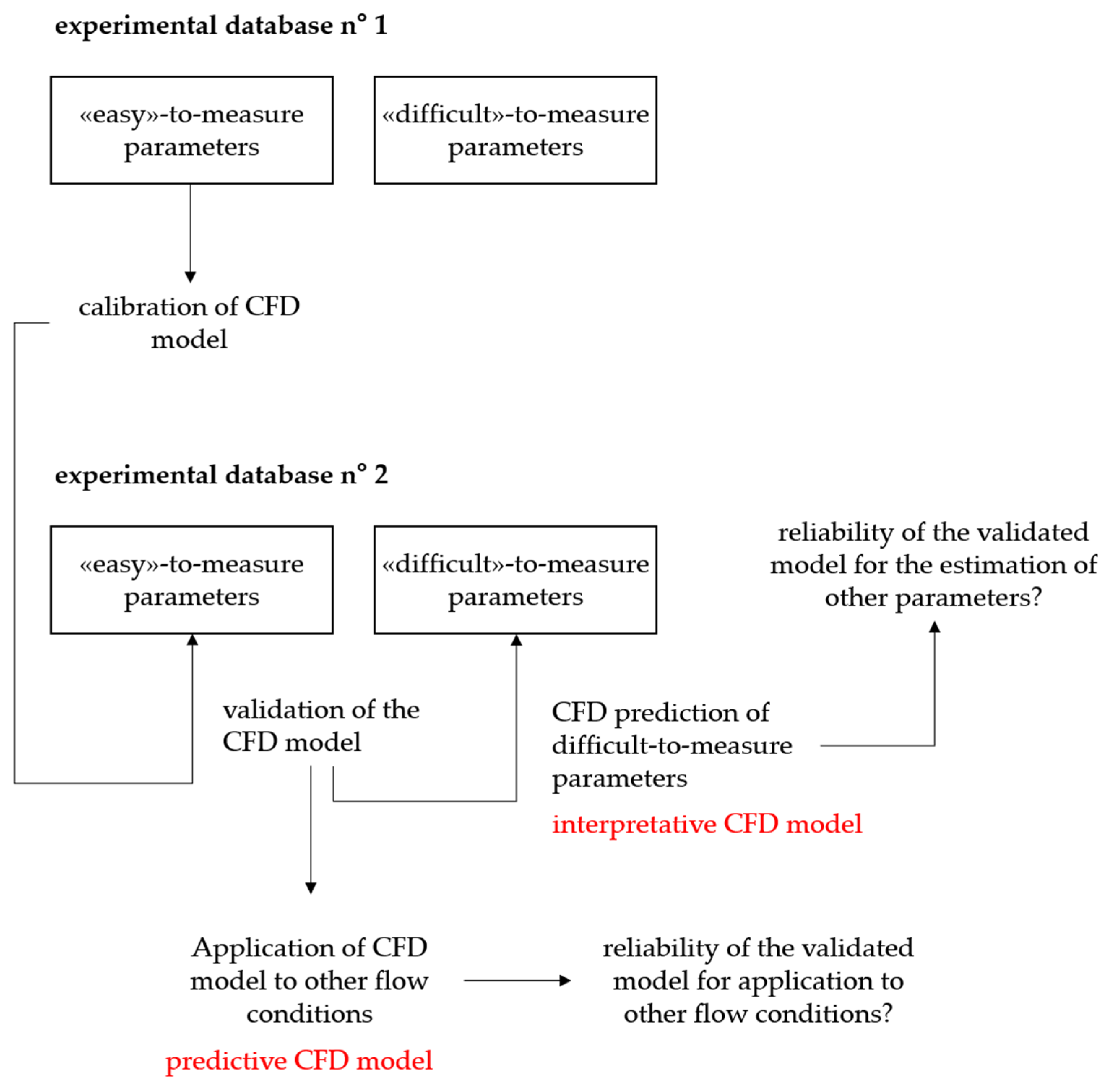
3. Sources of Uncertainty in the CFD Modelling of Slurry Flows

Regardless of the specific modelling approach employed, CFD simulations are characterized by several factors which produce uncertainty in the numerical solution, making it very challenging to prove that a certain model has a real predictive (but also interpretative) capacity. A possible classification of the sources of uncertainty is between numerical factors and modelling factors, subject of discussion in separate subsections.

3.1. Numerical Features Producing Uncertainty

Numerical factors are all features of the CFD model that can be controlled a priori, without the need of comparing the numerical solution with experimental data. As the name itself says, the numerical factors mainly include features of the CFD model related to the numerical solution of the equations.
Generalizing what is mentioned in Section 2.1 for the modelling of the fluid phase in the Eulerian–Lagrangian calculations, it might be stated that all equations with an Eulerian formulation are solved using grid-based methods like the Finite Volume Method, the Finite Element Method, the Finite Difference Method [42,73], etc.
In this regard, an important role is played by the computational mesh used to discretize the space domain. The discretization of the domain into cells or nodes gives rises to a deviation from the exact solution called grid discretization error. The discretization error can be estimated heuristically by running the same simulation on different meshes and looking at the effect of mesh refinement on a given target parameter, or quantified by formal protocols, like the Grid Convergence Index (GCI) analysis [74]. Indeed, an effective grid-independence study might not be straightforward task to accomplish: for instance, quantifying the degree of mesh refinement in the case of complex domains with heterogeneous cells distribution might not be easy; additionally, and at least in principle, proving the grid independence of a given set of target parameter does not imply that other features of the CFD solution are grid-independent as well; finally, constraints on the space mesh configuration are imposed also by the specific modeling approach (e.g., if a wall function is used, the size of the near-wall mesh should be consistent with the applied law; in Eulerian–Lagrangian models based on the point-particle approximation, as well as in volume-averaged Eulerian–Eulerian models, the size of the cells must be much bigger than the physical size of the solids, etc.). However, apart from these considerations, the point is that the assessment of the grid independence requires only numerical results, and, indeed, this must be achieved before comparing the CFD solution with experimental data.
In unsteady-state simulations, the effect of time discretization must be taken into account alongside space discretization. In principle, the smaller the time step is, the more accurate the solution is. However, the chosen time step must be also consistent with the turbulence modelling approach used. For instance, in the U-RANS modelling, the averaged equations are obtained from a moving average window whose width T is much larger than those of the turbulent fluctuations and much smaller than the time scale of the macroscopic flow (Section 2.1, Equation (6)), and this sets bounds to the discretization time step. Additionally, mesh size and time step are often related to each other and with the flow velocity through constraints on the Courant number, depending on the time discretization scheme [73]. Finally, in unsteady-state Eulerian–Lagrangian models at least two different time steps come up, and must be controlled by the user; these are the fluid time step associated with the Eulerian fluid flow equations, and the time step for the integration of the Lagrangian equations of motion of each parcel.
Other numerical sources of uncertainty are the differencing schemes for space and time discretization and the criteria for assessing the convergence of the solution algorithm. Indeed, all these features are strictly related to each other, as well as with mesh size and time step(s). For instance, grid independence can be obtained with a coarser mesh if higher-order space discretization schemes are used. CFD codes employ iterative solvers to solve the nonlinear discretized equations, which can be either coupled or sequential (e.g., SIMPLE, etc.). In order to understand whether convergence is being reached, reference is made to the normalized whole-field residuals, which are basically a measure of the local imbalance of each conserved variable in each control volume. The normalization factors are different among the CFD codes: for instance, in Ansys Fluent, all normalized residuals are approximately one at the first iteration, whereas in PHOENICS the normalization is based on the total inflow of the variable in question, and, therefore, they are much different from one at the beginning of the computation. In general terms, after an initial transient, all (normalized) whole-field residuals should decrease and tend asymptotically to zero. When all curves fall below a certain threshold, defined by the user, the solver stops and the simulation is terminated. In unsteady-state simulations, the residuals must fall below the threshold value at each time step, and this requires defining a sufficient number of iterations per time step: clearly, the smaller the time step size, the lower the number of iterations required per time step. Note that the trend of the whole-field residuals alone might not be a suitable indicator of convergence; in the case of two-way coupled Eulerian–Lagrangian models, for instance, whenever the coupling terms in the fluid flow equations are updated, the whole-field residuals are likely to increase suddenly, but this does not necessarily mean that the simulation is diverging. In these cases, convergence might be assessed, for instance, by monitoring the time evolution of significant local or global variables, such as the pressure drop over a certain pipe length, and verifying that these quantities tend to stabilize.
Another couple of numerical factors shall be included in this discussion. The first is the number of injected parcels in Eulerian–Lagrangian simulations. As discussed in Section 2.1, in Eulerian–Lagrangian simulations the number of calculated trajectories does not correspond to the actual number of physical particles in the system, but to the number of computational particles (or parcels), which is much lower. The number of physical particles that a parcel represents is independent of the actual solid concentration, and it is decided by the user based on the criterion that the number of calculated trajectories must be high enough to obtain significant statistics on the motion of the solids. Therefore, the number of injected parcels must be decided following a procedure that appears conceptually similar to a grid-independence study; that is, the number of trajectories is progressively increased until some reference target parameter (e.g., the statistics of the parcel–wall impingements in erosion calculations) becomes relatively stable.
Although it is not related to the solution algorithm, the last numerical factor belongs to this category in a broad sense, as it can be assessed from simulation results alone. This is the length of pipe that must be simulated to produce fully developed conditions in slurry pipe flow simulations. It is already explained that two different schemes of boundary conditions can be applied, namely, periodic boundary conditions with imposed mass flux, and inlet–outlet conditions (Figure 7). Clearly, talking about a length for flow development makes sense only if the inlet–outlet scheme is applied, and the value of such length depends on the distributions of flow variables imposed at the inlet boundary (e.g., uniform, piecewise linear, polynomial, etc.). The length for flow development might be easily established by comparing the solution of the CFD model on different sections of the pipe [36,75], or by inspecting the streamwise profile of different solved variables [57]. Recent studies indicated that, if uniform concentration and velocity distributions are applied at the inlet section, the length of the domain must be at least 100 pipe diameters long to achieve fully developed conditions [57].
The sources of uncertainty discussed so far are summarized in Figure 10 for the three main modelling approaches.

3.2. Modelling Features Producing Uncertainty

Once the inaccuracy of the CFD results induced by the numerical factors is properly controlled, the modelling sources of uncertainty come into play. At least practically speaking, no criterion exists to decide the value of these modelling factors other than the degree of agreement with experimental data, and, for this reason, they are probably the most critical feature of engineering computations in general, and of particle-laden flow simulations in particular. A significant example of modelling sources of uncertainty in single-phase RANS-based modelling is the turbulence model. The user of a CFD code is required to select a turbulence model among several options, which, in turn, include different settings. Although some general guidelines are available to select one model or avoid another (e.g., it is well-known that the k - ε standard model does not perform well in the case of pipes with rectangular cross sections, for which a Reynolds Stresses type model is a preferred option), very often the choice is reduced to finding the turbulence model which produces the best agreement with experimental data. This happens because, in the end, all turbulence models feature a certain degree of empiricism, and the calibration conditions of their many coefficients are often unspecified or unknown to users.
The number of modelling factors, and their impact on the CFD solution, is considerably higher for particle-laden flow models compared to single-phase models. The main modelling sources of uncertainty are discussed hereafter for the three main categories of CFD models for slurry flows.

3.2.1. Modelling Sources of Uncertainty of Eulerian–Lagrangian Models

In the case of Eulerian–Lagrangian models, sources of uncertainties for the fluid phase basically reduce to the turbulence model, including the near-wall treatment method (wall function approach versus low-Reynolds approach). However, several factors come into play in the Lagrangian modelling of the solid phase: for instance, in models based on the point-particle approximation, the forces acting on a parcel are obtained from force models, such as drag force, pressure gradient force, lift force, virtual mass force, etc. (Section 2.1). Each force model involves one or more force coefficients, which are obtained as a function of fluid dynamic and other parameters evaluated through a number of empirical correlations. For instance, even for the ideal case of a single, perfectly spherical particle, there exist several formulas expressing the drag coefficient as a function of the particle Reynolds number (Figure 11). The formula by Schiller and Naumann [76] is probably the most widely used in particle-laden flow simulations, followed by that of Dellavalle [77]. The standard drag curve of Clift et al. [78] consists of ten correlations for different ranges of R e p , and it provides an accurate representation of the behavior of the experimental data. All other curves shown in Figure 11 refer to empirical formulas listed in the textbook of Clift et al. [78], which, however, do not cover all available literature. The correlations appear quite similar with each other when depicted in a log–log plot of C d vs. R e p . Nonetheless, the differences in the values of C d might be non-negligible. For instance, at R e p equal to 100, the drag coefficients predicted by the formulas of Shiller and Naumann and by the standard drag curve is around 1.1, whereas the estimate of Dellavalle’s formula is around 1.25. It is difficult to establish a priori the impact of such change in C d on the final simulation results, but surely the user of a CFD code must be aware that using a drag coefficient correlation instead of another might result in more or less accurate predictions.
The situation is even more complex because, unlike the spherical glass beads used in some experiments, natural solids like sand are not spherical in shape; therefore, using any of the correlations in Figure 11 might not be appropriate. One of the most widely used formulas (although not the only one, see [79]) for evaluating the drag coefficient of non-spherical particles is that of Haider and Levenspiel [80], which expresses C d as a function of both R e p , defined in terms of the diameter of the volume-equivalent sphere, and a particle spherical coefficient, φ , which is the ratio between the surface area of the volume-equivalent sphere and the actual surface area of the particle. The Haider and Levenspiel correlation was obtained empirically by interpolating experimental data concerning artificial solids, which are either isometric particles with φ 0.50 and disks with φ 0.23 . In the case of natural solids, φ is very difficult to quantity in spite of its precise geometrical definition, because the value of φ will be different for every single grain. In this case, reference can be made only to macroscopic classifications and general guidelines reported in the literature, such as φ equal to 0.66, 0.76, and 0.86 for sands with fully-sharp, nearly rounded, and highly rounded grains, respectively [81]. Figure 12 shows the Haider and Levenspiel curves for such three values of φ , clearly indicating that, for a given particle Reynolds number, the drag coefficient of non-spherical particles is higher than that of spherical ones, especially for moderate and high values of R e p . A priori, it is difficult to quantify the actual impact of ignoring the effect of particle shape on the drag coefficient (which means, for instance, to simply employ the Schiller and Naumann’s formula even in the case of natural sands) on the output of a CFD simulation, as the degree of inaccuracy appears problem-dependent. Nonetheless, the user of a CFD code should be aware that, in principle, using one value of φ instead of another might produce different results, and, therefore, φ and more generally the modelling of particle shape for natural materials is a significant source of uncertainty in the simulation of slurry flows.
Indeed, the drag force is generally the dominant one in slurry flows, but also other forces can play an important role in specific conditions; therefore, also the values of the other force coefficients (e.g., lift coefficient, added mass coefficient, etc.) may be listed among the modelling factors affecting the reliability of a CFD model. In this regard, it might be observed that, in point-particle simulations, particle shape is usually accounted for only by modifying the drag coefficient, as allowed, for instance, by the correlation of Haider and Levenspiel [80]. However, models derived for perfectly spherical particles are applied to all other force coefficients. Such approximation, forced by the lack of suitable general and applicable models, might produce errors depending on the flow subject of investigation and the scope of the CFD simulation. The user should be fully aware of this.
Focusing, once again, on the solid phase side of the Eulerian–Lagrangian models, other critical factors are related to the modelling of the particle–particle interactions (in four-way coupled models only) and of the particle–wall interactions. As briefly mentioned in Section 2.1.2, several particle–particle interaction models exist and are available to CFD users. For instance, the widely-used Ansys Fluent code provides four embedded options for normal contact (spring, spring-dashpot, Hertzian, Hertzian-dashpot), and two embedded options for tangential contact (friction-dshf, friction-dshf-rolling), and all these sub-models, in turn, depend on coefficients which are not easy to quantify.
As far as the particle–wall interactions are concerned, these processes are typically modeled via two restitution coefficients, e n and e t , which relate the normal and tangential parcel velocity before and after an impact against the wall boundary (Figure 8a). In slurry erosion simulations, where the modelling of the impacts between the particles and the solid walls is of utmost importance, use is generally made of empirical correlations expressing e n and e t as a function of the parcel–wall impact angle, θ P , imp . Commonly correlations of this type are that by Forder et al. [82] and the stochastic rebound model by Grant and Tabakoff [83], graphically depicted in Figure 13. Although the two models present qualitative similarities, the differences in the estimated values of e n and e t might be significant, producing different behavior of particle trajectories after the first impacts. Additionally, the modelling of the particle–wall interactions in the Eulerian–Lagrangian framework is even more problematic because, as already mentioned: (i) the role of the wall roughness on particle rebound might be significant, and it requires specific modelling approaches to be accounted for [50]; (ii) there exist other types of interactions in addition to the impacts [51].
The discussion above highlighted that, in the Eulerian–Lagrangian modelling, there exists several sources of uncertainty related to the calculation of the fluid flow field and the tracking of the parcels’ trajectories. Actually, two other modelling features shall be added. The former is the type of coupling between the phases. It was already observed in Section 1.3 that, according to well-established classifications [28,29], the coupling regime between in a particle-laden flow was related to the volumetric concentration of the solids. Nonetheless, the traditional criteria in Figure 3 are difficult to apply in practical slurry flow simulations, primarily because they would require to know the detailed solid volume fraction map before running the calculations, and also because they involve very low values of solid volume fraction, and, therefore, appear “too conservative” when the carrier fluid is a liquid. As a result, some more practical approach is often employed, especially in slurry erosion studies, which consists in assuming one-way coupling even up to solid volume fractions of about 1%. Messa and Malavasi [84] found that the erosion depth profile produced by a normal slurry jet with 0.5% volumetric concentration does not practically change if the two-way coupling sources are included in the momentum equation of the liquid phase. However, up to the authors’ best knowledge, no systematic investigation of these aspects has been published yet, suggesting that the coupling regime assumed in slurry flow simulations is not always physically justified, and, therefore it is a choice of the user which might produce errors depending to the scope of the simulation. Finally, in slurry erosion simulations, an important modelling factor is represented by the erosion models used to turn the parcel–wall impact characteristics into an estimate of the material removal. Most erosion models are algebraic formulas that express the mass loss associated with a parcel–wall collision as a function of several parameters, such as the modulus of the parcel velocity at the stage of impingement, v P , imp , the parcel–wall impact angle, θ P , imp , as well some variables related with the abrasive particle and the eroding material (Figure 8a). These formulas are empirically obtained by fitting the experimental results of dry direct impact tests, in which an air–solid jet exiting a nozzle impinges at high velocity against a sample of the selected target material. The rationale behind these models is that the motion of the particles in air is dominated by their inertia and, therefore, the impact velocity and the impact angle are the same for all particles, and are approximately equal to the easily measurable particle velocity at the nozzle exit and nozzle-to-specimen inclination angle. Several erosion models of this type have been proposed throughout recent decades (see [85,86] for a review), and some of them are also embedded as built-in options in multi-purpose CFD codes. Indeed, models of this type, such as the widely used Oka’s [87,88], are formally simple and easy-to-implement, but they suffer from a relatively high number of not well characterized numerical coefficients. Additionally, their limits of validity are often unspecified, or simply unknown to users; therefore, erosion models are frequently misapplied, yielding estimates of doubtful validity. At the other extreme, there is the fully physically-based modelling of erosion, in which the description of the particle–wall impacts is carried out by solving for the fundamental laws of damage mechanics. Such an approach appears indeed the most valuable, but it has a severe limitation in the high computational cost, mainly arising from the multi-scale nature of the processes to be simulated, i.e., from the relatively large scale of the particle-laden flow to the micro-scale of the individual particle–wall impacts. Although the recent findings of Leguizamón et al. [31] are a valuable avenue for future research, we are still not ready for fully physically-based modelling of slurry erosion in engineering computations. Finally, in between the fully empirical and the fully physically-based approaches, there exists a third way, represented by the phenomenological erosion models. These models are obtained from a simplified description of the erosive damage produced by a particle–wall impingement; in spite of a certain physical foundation, they include difficult-to-characterize or simply difficult-to-measure parameters, so that, in the end, they have strong empirical content. Pioneering studies in the field of impact erosion modelling rely on such a phenomenological approach [89,90,91] and, even if these models are still used at present, they do not allow for a higher degree of confidence compared to fully empirical correlations. In summary, a significant source of uncertainty in slurry erosion calculations (if not the most significant) is given by the erosion model. This has been well documented, for instance, by Messa and co-workers [84]. An engineering effective compromise solution to overcome the inaccuracy of empirical comprehensive formulas taken from the literature and the high computational cost of a fully physical approach was the subject of the research work of different authors in the last ten years [92,93,94]. Such a method, which will be discussed in Section 4.3, consists in combining CFD and experimental results for highly accurate calibration of case-specific erosion models in slurry erosion calculations.

3.2.2. Modelling Sources of Uncertainty of Two- and Multi-Fluid Models

Several modelling sources of uncertainty come into play in Eulerian–Eulerian models. An important role is played by the constitutive equations of the solid phase, namely, the models for the two viscosity coefficients, μ s and λ s , and for the solids pressure. It was explained in Section 2.2.2 that two main categories of Eulerian–Eulerian models exist, namely, those which employ closures from the Kinetic Theory of Granular Flow (KTGF), and those relying on empirical closures. Although KTGF-based closures are more physically based in nature, different alternative formulations are available and have been employed for the simulation of slurry pipe flows, as will be further discussed in Section 4.4. Additionally, all closure equations involve parameters and coefficients which are not fully characterized yet simply difficult-to-quantify, and act as potential sources of uncertainty: among others, the restitution coefficient of particle–particle collisions, the radial distribution function, the maximum packing volume fraction, the specularity coefficient, the angle of internal friction of the solids, etc. Additionally, two-fluid models based on empirical constitutive equations include sources of uncertainty. For instance, if the solid viscosity, μ s , is obtained from the viscosity of the mixture, μ m (Equation (31)), then the use of a certain correlation for μ m instead of another, as well as the values assigned to the coefficients in each correlation, might produce significantly different CFD results. Similar considerations can be made regarding the use of the empirical correlations relating the solids pressure to the spatial gradient of the solid volume fraction [39,54]. Sometimes, the solid pressure is simply taken equal to the pressure of the carrier liquid, as in the β-σ two-fluid model of Messa and Matoušek [57]; note that, even if no coefficients are introduced, this option does not reduce the number of modelling factors, as it brings an uncertainty associated with the assumption p ˜ s = p ˜ l .
From a certain point of view, the evaluation of the exchange of momentum between the two phases is more critical in the Eulerian–Eulerian framework rather than in the Eulerian–Lagrangian one. The formal similarity between the f ˜ l s term in the Eulerian–Eulerian model (Equation (37)) and the fluid–particle forces in the Lagrangian equation of motion (Equation (17)) is already underlined, and it was remarked that the modelling of the two items is carried out in a similar fashion by replacing the particle-related quantities with the volume-averaged ones. Therefore, it is not surprising to see that the same sources of uncertainty discussed for the Eulerian–Lagrangian models (e.g., which forces must be included? How to evaluate the force coefficients? How to account for the effect of particle shape on the force coefficients?) are present also in the Eulerian–Eulerian models. However, another source of uncertainty characterizes most two-fluid models, namely, the method used to include the effect of the solid volume fraction in the evaluation the drag coefficient, C ˜ d . The basic idea is that a particle in a slurry mixture experiences a higher resistance to flow compared to the case in which the same particle travels alone in a pure liquid. From a modelling point of view, this effect might be accounted for in three ways. The first option is to modify the definition of the particle Reynolds number by replacing the viscosity of the fluid with the viscosity of the mixture, μ m , or some formally analogous parameter. This method was introduced in Ishii and Mishima [95], and, with a different characterization, it is the basis of the β-σ two-fluid model of Messa and Matoušek [57]. The second option is to multiply C ˜ d by an empirical coefficient depending on the solid volume fraction, e.g., the correction factor of Di Felice [96], which was used by Messa and Malavasi [66] to simulate the slurry flow in vertical pipes at moderate concentration. Finally, the third option is to employ alternative drag coefficient correlations which have been specifically developed for the entire range of solid concentrations, such as that proposed by Gidaspow [97], employed by Ekambara et al. [36] to model the slurry flow in horizontal pipes. As a final remark, it is noted that, although the concentration-related corrections have been mostly incorporated into Eulerian–Eulerian models, the same methods might be also employed in the Eulerian–Lagrangian models, if the solid volume fraction is high enough. This has been carried out, for instance, in [98,99]. Regardless of the modelling framework, the application of the methods discussed so far introduces uncertainty to the numerical solution, as it increases the number of uncertain sub-models, parameters, etc.
The degree of uncertainty of the solution of Euler–Euler models is further enhanced in the case of turbulent flows. As was explained in Section 2.2.4, the double-average approach produces long equations, which, in order to be practically solved, need to be simplified by neglecting some critical terms which are particularly small or simply difficult to evaluate. Although the choice of neglecting some terms in the equations might be the result of some physical considerations, this is not always the case, especially because two-fluid models are intended as tools to simulate a large class of flows, and claiming a priori that some terms are much smaller than the others might not be possible. Even if the attention is restricted to the terms which are usually not neglected, the choice of using a certain closure instead of another might sometimes look arbitrary. For instance, the gradient diffusion approximation (Equation (46)) is an effective way to model the double correlations between the fluctuating velocity vector and the fluctuating volume fraction, but does not have a real physical justification for inertial particles. Additionally, in the case of slurry flows, it makes some features of the CFD solution (such as the concentration distribution of slurry pipe flows) dependent upon the value of the turbulent Schmidt number for volume fractions, σ , which is not well characterized and often simply taken as tuning coefficients. A similar situation holds for the double correlations between the fluctuating velocity components of the two phases: when modeled via Boussinesq-like approximations, uncertainty arises from the modelling of the two eddy viscosities. Note that, as already observed for the solid pressure, not including the eddy viscosity of the solid phase, as in most KTGF-based models, or taking the eddy viscosity of the solid phase equal to that of the liquid phase, does not reduce the number of numerical factors. The two examples here above, in fact, are in themselves modeler’s choices which carry some uncertainty.
Finally, a key modelling feature in the Eulerian–Eulerian framework is represented by the wall boundary conditions of the solid phase. The choice of a type of boundary condition instead of another has proven to have a significant impact, for instance, on the predicted hydraulic gradient in slurry pipe flow simulations [100,101]. Additionally, even once the type of wall boundary condition is defined, an inappropriate definition of the coefficients in the boundary law can affect the reliability of the CFD predictions: this is the case, for instance, of the partial slip condition of Johnson and Jackson [71], which is widely used in KTGF-based models and depends on the specularity coefficient, a parameter which appears crucial and difficult-to-decide [102].
Clearly, the number of modeling factors coming into play in the multi-fluid model is considerably higher than for the two-fluid model, owing to the presence of multiple secondary phases. However, these factors are not different in nature compared to those discussed so far. Each secondary phase, in fact, requires its own constitutive equations and boundary conditions, and the momentum exchange between all pairs of phases must be accounted for. The amount of difficult-to-decide coefficients, parameters, and sub-models makes it very hard to control the numerical solution accuracy, and, therefore, to gather some confidence in the predictive capacity of the multi-fluid model.

3.2.3. Modelling Sources of Uncertainty of the Mixture Model

Additionally, the mixture model was developed starting from the two-fluid model, and therefore, it brings along similar, yet more limited in number, modeling factors. Particularly, critical sources of uncertainty include the constitutive equation for the stresses tensor of the mixture, · τ m , and the modelling of the Reynolds-like stresses term of the mixture, · τ m t , of the diffusivity coefficient D ls used to account for the effect of the turbulent fluctuations on the relative velocity, and of the drag coefficient, C d . Manninen et al. [35] reported that the three different modelling strategies to account for concentration effects on C d in Eulerian–Eulerian models previously described (namely, evaluating the particle Reynolds number with respect to μ m , applying a correction factor depending on Φ s , or using specific drag coefficient correlations) can be used also in the mixture model. However, these strategies have been rarely employed in previous numerical investigations on slurry pipe flows [103], probably also because the Ansys Fluent code, which is the most widely used, does not embed any of them. With regard to · τ m , the most common choice has been the KTGF approach, available as an option in Ansys Fluent, which requires evaluating the viscosity of the solid phase through some KTGF-based correlation, thus taking along all uncertainties discussed for the two-fluid modes. To the authors’ best knowledge, in slurry pipe flow simulations the direct evaluation of μ m as a function of Φ s has been explored only by Hu and Guo [103], who used the correlation for μ m developed by Moody to describe the rheology of colloidal solutions of very small spherical particles suspended in a liquid [104]. Finally, mixture-based wall functions are usually applied as wall boundary conditions for the momentum equation of the mixture. Nonetheless, alternative modelling approaches are desirable, since it has been shown by Kaushal et al. [67] that this option might produce severe overestimation of the hydraulic gradient of fine sand slurry flowing in horizontal pipes at high concentrations.

3.2.4. Summary and Recommendations

Figure 14 summarizes the most significant “modelling” sources of uncertainty of the three main modelling approaches for the simulation of slurry pipe flows. In order to give confidence in the numerical predictions, the user should pay attention to the choice of all these features of the CFD model, trying to employ a combination of sub-models and coefficients which proved applicable to the case study under investigation. If no information is available to decide whether a certain combination is more appropriate than another, maybe because the applicability limits of some closures and correlations are unknown, it is recommended to carry out a sensitivity analysis to assess which feature of the CFD solution is affected by each “uncertain” sub-model and coefficient, and to what extent. This will allow a rough idea of the level of confidence of the numerical predictions.

4. Review of Previous Investigations

4.1. Overview of Published Literature

To the authors’ best knowledge, the first publications on the CFD modelling of slurry pipe flows date back to the 1980s, these pioneering studies being carried out by M.C. Roco, C.A. Shook, and co-workers from the University of Kentucky. In total, we were able to find 86 research articles published in scientific journals, limiting the analysis to studies showing an application to settling slurry flows in pressurized pipes. Most of these 86 articles are high-quality works and will be reviewed in the following subsections. Conversely, other articles will not be referenced since, according to the authors’ opinion, they provided only a limited contribution to the state-of-the-art. Nonetheless, the statistical considerations reported hereafter are based on the whole population of papers. In fact, the scope of the analysis presented in this section is to reflect the research trends rather than to illustrate the big steps forward, which will instead be the topic of the following sections.
A preliminary observation could be made in terms of the number of articles per year, which is constantly increasing. Only 13 papers out of the total 86 were published before 2000. During the first decade of the 21st century, every year, only one to two articles were published on the CFD modelling of slurry pipe flows, and this number was tripled during the 2010s. In 2020 alone, nine papers were published on this topic. The increase in the amount of literature is not surprising, as it might be easily correlated with the advances in computer power and the widespread use and capabilities of multipurpose CFD codes. However, as already mentioned, not all these papers have represented a real advancement over the state-of-the-art.
Interesting statistics can be made by classifying the 86 papers according to different criteria:
  • Firstly, regarding their topic. A total of 69 articles, corresponding to about 80% out of the total 86, concern the modelling of particle transport in slurry pipelines, generally at a high solid volume fraction. Conversely, the remaining 20% are focused on slurry erosion of pipeline components, typically pipe bends, at moderate solid concentration.
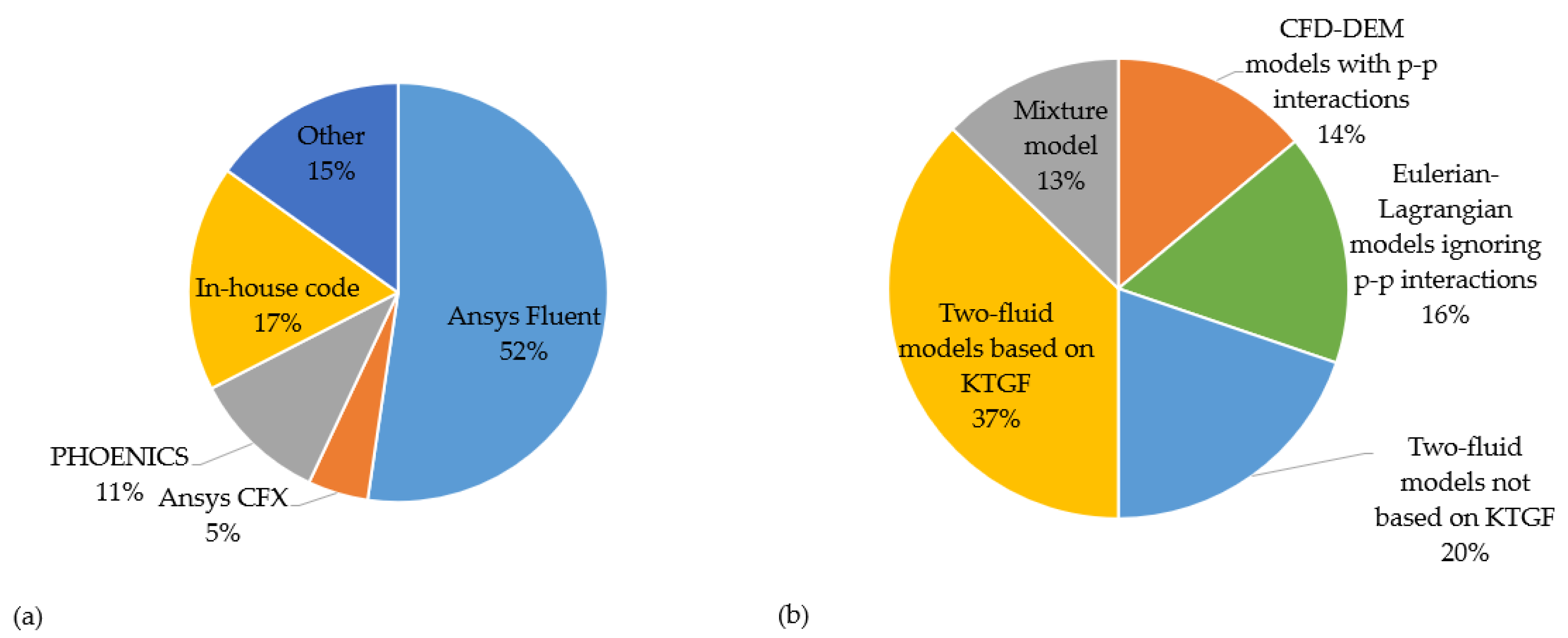
  • Secondly, regarding the software used. As shown in Figure 15a, more than half of the investigations were performed using the Ansys Fluent code, which embeds all types of models described in Section 2; other commercial codes used were PHOENICS and Ansys CFX. A significant fraction (≈17%) of the numerical studies were performed using in-house codes, which mostly applies to the pioneering investigations. The category field “other” in Figure 15b include papers in which the use was made of a combination of different open source or commercial software, as well as those where no information was provided.
  • Thirdly, regarding the modelling approach. As shown in Figure 15b, Eulerian–Lagrangian models, either including or ignoring particle–particle interactions, were used in around 30% of the total published articles, indicating that the Eulerian approach is the preferred one for the modelling of slurry pipe flows. However, the data must be interpreted in the light of the topic of the study: in fact, almost all papers concerning slurry erosion used the Eulerian–Lagrangian models, whereas the slurry transport at high concentrations has been rarely simulated using this approach. It is also interesting to underline the relation between the type of modelling approach and the used software: for instance, almost all investigations using two-fluid models based on KTGF and those using the Mixture Model were performed with Ansys Fluent. Conversely, although particle–particle interaction models are embedded in most commercial codes, CFD-DEM simulations have been usually run by coupling different codes, or with a single in-house package.

4.2. Studies Using Eulerian–Lagrangian Models for Predicting Particle Transport

Starting from the considerations outlined in the previous sections, it is not surprising to see that only a few studies dealt with the hydraulic pipe conveying of slurries in Newtonian liquids using the Euler–Lagrange approach. The high values of solid concentration typical in slurry pipelines make it unreasonable to neglect particle–particle interactions, and, therefore, these studies belong to the unresolved group of CFD-DEM modelling. The high computational cost of this modelling approach is probably the main reason behind the small number of published articles, but it might be noted that the latest releases of widely used commercial CFD codes embed particle–particle collision models. This, in addition to the increase in the capability of computers, might explain why, only in 2020, four papers have been published on the CFD-DEM modelling of slurry pipe flows. Hereafter, four relevant works, published between 2013 and 2020, will be referenced [105,106,107,108].
In 2013, Capecelatro and Desjardins [105] investigated liquid–solid slurries in a horizontal pipe for operating conditions above and below the critical deposition velocity. They used a high-fidelity large eddy simulation combined with Lagrangian particle tracking solver. The slurry consisted of sand particles of a diameter ranging from 50 to 307 μm (mean particle diameter was 165 μm) suspended in water. Both the sand and water were fully coupled via volume fraction and momentum exchange terms. Particle–particle and particle–wall collisions were modelled using a soft-sphere approach proposed by Cundall and Strack [109]. The pipe geometry and particle size distribution corresponded to experimental data from Roco and Balakrishnam [110]. The pipe diameter was 0.0515 m with a mean particle volume fraction of 0.084. Periodic flow conditions were enforced in the flow direction (Figure 7a). A domain aspect ratio (= length of simulated domain/pipe diameter) of 5 was chosen, resulting in over 16 million particles and 18.7 million grid cells. Cell size is approximately equal to the maximum particle diameter. Two bulk velocities were considered, case A with a bulk velocity of 1.6 m/s and case B with a bulk velocity of 0.83 m/s. Experimental data of particle concentration, velocity distribution and frictional pressure drop were available for case A only. Comparison of experimental and numerical data showed a very good agreement for particle velocity profiles along the vertical axes. A slight over prediction of particle concentration close to the pipe bottom was observed. The computed pressure drop was about 20% lower compared to the experimental data. In this study, the Eulerian–Lagrangian model was used to gather information on features of the flow that are hard, if not impossible, to measure experimentally. According to the classification presented in Section 1.3, the model provided an interpretative framework.
In 2015, Arolla and Desjardins [106] studied the physics of turbulent liquid–solid slurry flow through a horizontal periodic pipe. They used the same numerical strategy as Capecelatro and Desjardins [105]. In this simulation, the pipe geometry and sand particle diameter corresponded to experimental data from Dahl et al. [111]. The pipe diameter, particle size and domain aspect ratio were 0.069 m, 280 μm and 3.75, respectively. The size of computational cells was equal to 1.57 times the particle diameter. Due to the high computational costs, the simulations were restricted to three cases whose Reynolds number varied from 20,700 to 41,400. Two cases were below and one over the critical deposition velocity. The simulation with the smallest velocity and the largest number of particles (19.25 million) took approximately one million core hours and was typically run on 500 computer cores. The CFD model was able to predict the change in flow regime occurring for increasing liquid flow rate. At low liquid flow rates, the sand will drop out of the carrier liquid and forms a stable, stationary bed. When the liquid flow rate increases above a specific value, sand starts getting transported in a thin layer above the bed. As the flow rate increases further, the sand bed breaks into a series of slow-moving dunes which eventually form a moving bed along the bottom of the pipe. At even higher flow rates, the sand particles get fully suspended in the carrier liquid.
In 2018, Uzi and Levy [107] investigated the flow characteristics in horizontal hydraulic conveying of coarse particles in terms of operating conditions via Euler–Lagrange approach. The range of investigated concentration extended up to C vi = 0.30, and two solid materials and two carrier liquids were considered. The first set was silica-sand particles in water with respect to the experimental data of Gilles and Shook [13]. A pipe diameter of 0.053 m and the periodic boundary condition scheme with a domain aspect ratio of 10 were used. The size of sand particles varied from 2.3 to 2.5 mm. A calibration was performed through the particle–wall friction coefficient, which appears in the modelling of the particle–wall collisions in the DEM framework, and was tested in the range 0.15–0.6. The authors claimed that the smallest deviation from the experimental measurements was observed for the particle–wall friction coefficient equaled 0.2, but they did not specify which target parameter was considered. This value was chosen for all simulations. The deviation from the measured and simulated hydraulic gradient was up to 11%. The second pair of materials was salt particles transported by brine. For this suspension, a detailed analysis was carried out to understand how the operating conditions (conveying velocity, particle concentration, particle size and pipe diameter) impact the flow patterns. The coupling scheme between the particles in in-house DEM code and the CFD software was performed through a User Defined Function into Ansys-Fluent v17.2 (Ansys Inc., Canonsburg, PA, USA).
In 2020, Zhou et al. [108] presented a numerical study of the horizontal hydraulic transport of coarse sand particles in water by means of Euler–Lagrange approach. Following the experimental data of Gilles and Shook [13], the simulated horizontal pipe had a length of 4 m and a diameter of 0.0532 m. Three different mesh sizes (coarse—21,492 cells, medium—37,611 cells and fine—432,055 cells) were tested and the simulated distribution of solid volume fraction along vertical axes was compared to the experimental data for concentrations equal to 0.15 and 0.30. The acceptable deviation was achieved for medium and fine mesh, so the medium mesh size was finally chosen. It means that the cell dimension in the direction of the flow was about 20 mm and the average cross-section cell size was about 11.7 mm2. Although two particle diameters (2.4 and 3.5 mm) were reported to be tested, most results are related to the largest particle size. The investigated solid concentrations were 0.05 and 0.10. The CFD-DEM simulations were solved using an in-house code. The transition from the stationary bed flow, through the moving bed flow, to the heterogeneous suspension flow was presented and the simulated pressure drops were consistent with the published experimental data, but no quantitative comparison was made. During the transition from stationary bed flow to the heterogeneous flow the particle–particle and particle–wall forces firstly decreased and then remained nearly constant. The paper suggests that a RANS-based CFD-DEM can be used to predict the transition between slurry flow regimes, but further research and an extensive validation study is needed to give strength to this claim.
It can be said that the Euler–Lagrange approach makes it possible to gather insight into the flow not only at the local level, as characteristic of CFD in general (Section 1.3), but also at the scale of the individual particles. For instance, it allows obtaining information on the distribution of mean and fluctuation velocities of particles, the influence of individual size fractions in multi-size slurries on the flow characteristics. On the other hand, in addition to enormous computing power, it also requires knowledge of some parameters, such as the particle–wall and particle–particle friction and rolling coefficients, which act as “modeling” sources of uncertainty (Section 3.2.1). The published simulations use their own in-house codes, which are usually unavailable. In addition to the standard CFD-DEM model implemented in Ansys-Fluent, it is possible to use an Open Source Discrete Element Method Particle Simulation Software LIGGGHTS® (DCS Computing GmbH, Linz, Austria) and CFDEM® coupling Open Source CFD-DEM model (DCS Computing GmbH, Linz, Austria) working on Open Foam platform, which models the turbulent fluid flow by solving for the instantaneous Navier–Stokes equations (DNS approach). Such methodology was applied by Zheng et al. [48] to simulate the slurry of 2 mm glass beads in Glycerol solution for Reynolds numbers below 10,000 in a horizontal periodic pipe. The study presents a throughout validation in terms of concentration profile, and then the model was extensively used to find out difficult-to-measure features of the flow for the same conditions.
Some numerical simulations can be found in the literature [112,113], which partly fall both into the Euler–Euler and the Euler–Lagrange approaches. It is mostly a combination of EDEM and Ansys-Fluent software, where the coupling between solid and liquid phases is based on Euler–Euler modelling, while the motion of individual particles is realized in the EDEM program. In such cases, the volume information of the solid phase is more accurate than in a classical Euler–Euler approach.
In summary, it is clear that the CFD-DEM model has the potential to provide a great deal of insight into the pipe transport of solids in the form of slurry. However, up to now, the high computational cost has been a limiting factor to the use of this approach. Save for a few exceptions, in the published literature the CFD-DEM model has been employed with an interpretative purpose, without a clear assessment of the role played by coefficients and parameters, such as, for instance, those of particle–particle interaction models. Nonetheless, it is expected that the number of investigations will increase considerably in the future, as a result of the increase in computer power.

4.3. Studies Using Eulerian–Lagrangian Models for Predicting Slurry Erosion in Pipeline Systems

The present section deals with the use of CFD models to investigate the erosion damage of slurry pipelines. It will be arranged in three different subsections, dedicated to the characterization of the slurry erosion phenomenon, to the challenges in its modelling through CFD, and to the evaluation of the capability of the CFD approach based on the analysis of previous investigations.

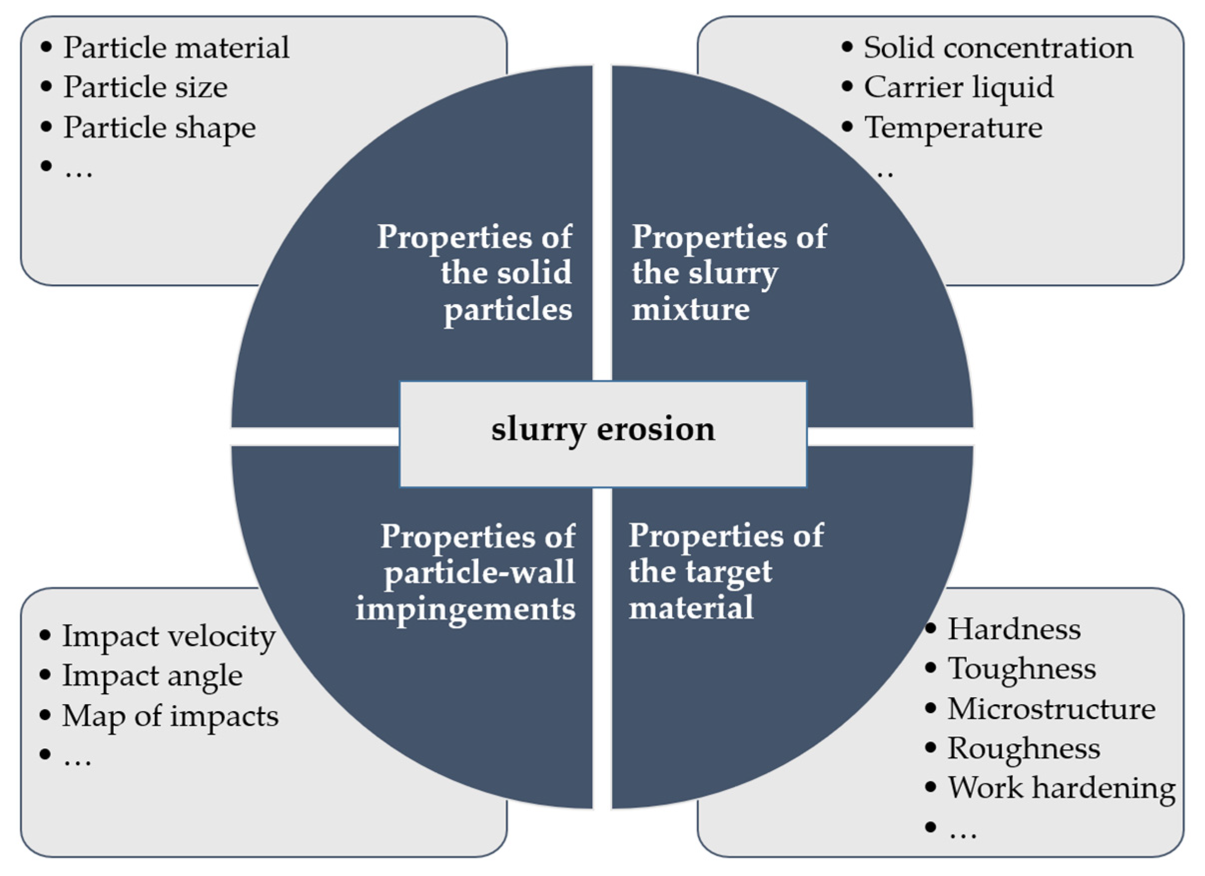
4.3.1. The Engineering Problem and Relevant Parameters

Erosion has always been a concern in pipeline systems, as it leads to serious financial losses caused by downtime, failures and equipment replacement costs [114]. There has been a growing interest in applying simulation for predicting failure and extending equipment life span, not only because of the costs and operational issues associated with in loco measurements, but also due to the lack of other models. However, even before proposing numerical equations/correlations, researchers need to understand the fundamental mechanisms of this complex failure mode. In this sense, models such as the ones described in this paper have proven very useful for proposing mitigation devices/techniques, and providing insight into the basic mechanisms involved [115,116,117,118,119].
Depending on its multiphase characteristics, a slurry can sometimes be classified as a highly viscous fluid. Naturally, it should be borne in mind that the rheological properties of a slurry can be affected by various other factors such as mass loading of the carried particles, particles shape, size and density and the properties of the conveying fluid.
Slurry transportation can involve corrosion, abrasion and erosion. Among these, the erosive process plays the most important role in total wear. Slurry erosion usually occurs under turbulent flow conditions when the moving slurry strikes a surface, scars it and removes material. It has to be remarked that as erosion and abrasion are both mechanical wear processes showing many similarities [114], they are sometimes confused with each other. However, the basic difference between the two is that erosion involves a transfer of kinetic energy from the impinging particle to the target surface, whereas abrasion is the loss of material due to the passage of hard particles over the surface without impingement. In erosion, the contact time between the erodent and the eroded surface is much shorter than in abrasion [120]. For a fully detailed review regarding the mechanisms involved in slurry erosion and experimental apparatus used, the reader is referred to [121].
In recent decades, many researchers quantified the effect of different parameters on solid particle slurry erosion. Often, e.g., in [121], these parameters are divided into four groups, i.e., the nature of the target surface, the nature of the erosive particles, the characteristics of the flowing slurry, and the contact or impingement condition (Figure 16).

4.3.2. Challenges in the CFD Modelling of Slurry Erosion

Although Euler–Euler models have also been applied in erosion simulations [122,123], Euler–Lagrange models still remain the workhorse. This is a natural consequence of the fact that erosion models are mostly empirical correlations of the erosion ratio as a function of the local particle velocity, angle of impact and collision frequency. These input parameters are naturally available from a particle simulation; therefore the EL approach constitutes the most obvious choice. Yet, some issues remain. For instance, in the classical EL approach, particles are assumed to be points. This assumption may be violated in the vicinity of walls, especially if a boundary layer refinement is applied in turbulent flows. Another important issue, already mentioned in Section 2.1.3, is that most CFD codes actually track the particle center. However, this allows for the particle to somehow cross nearly half-diameter outside of the flow domain. Although this might be considered as an artificial “softness”, it will incur errors when interpolating the fluid velocity to the particle center; thus, the impact velocity will be affected (Figure 8b). Because the erosion rate is normally a strongly non-linear function of the impact velocity, erosion predictions might be compromised. As shown by Messa and Wang [52], neglecting the finite size of the particle in wall collisions can significantly increase the wear prediction even for 50-micrometer particles. Fortunately, two alternatives are proposed by the former authors for fixing this without substantial modifications in existent codes. The more effective of the two, further developed in Messa et al. [94], consists in extracting from the point-particle trajectory the parcel position, velocity and angle half particle diameter away from the wall, and take these values as the parcel–wall impingement characteristics to be used in the erosion calculations. Another strategy to overcome the inaccuracy associated with the point-particle treatment of the parcel–wall impingements was proposed by Zhang et al. [124], which consists in employing different mesh sizes and different near-wall treatment methods according to the size of the particles.
More specifically, there have not been many articles on erosion simulations in slurry pipelines components. As already mentioned in Section 3.2.1, one of the most critical features of slurry erosion modelling resides in the approach used to turn the parcel-wall impact characteristics into estimates of material removal. In fact, on the one hand, empirical erosion formulas taken from the literature might produce at times highly inaccurate predictions. On the other hand, a fully, physically-based treatment of the material removal process will require very high computational costs. A compromise strategy has been developed, which consists in combining experimental data with CFD results to solve the associated inverse problem and generate high precision models of suspension erosion. Lester et al. [92] applied such a technique to a test case of silica sand particles eroding a cylindrical aluminum specimen (Figure 17a), and the resultant data were fitted to an erosion function.
This practical modeling philosophy is to consider models specific to a particular impact particle/material combination, such that the local average mass erosion rate per unit area, Φ e [kgeroded·m−2 s−1] is closely related to the concentration of particles (parcels) and particles (parcels) impact angle and velocity:
Φ e = Φ m F ( θ P , imp , v P , imp )
where Φ m is the local average particle impact rate [kgabrasive·m−2 s−1], v P , imp and θ P , imp are the parcel impact velocity and the parcel impact angle (Figure 8a), and F is a dimensionless wear function.
The application of such erosion models represents a regular forward problem; for a particular geometry, given the wear function F , and calculated particle impact rate Φ m , velocity v P , imp , and angle θ P , imp distributions of the material surface, what erosion distribution Φ e results?
Conversely, the determination of the wear function F from experimental data represents an inverse problem: for a particular experiment given the calculated particle impact rate Φ m , velocity, v P , imp , and angle θ P , imp distributions, what function F (or possible set of functions) generates the observed erosion distribution Φ m ? In this context, Lester et al. [92] obtained the distribution of erosion rate intensity, Φ e , as a function of the erosion depth at time t , η ( t ) [m], as follows:
Φ e = ρ t · η ( t ) t
where ρ t [kg·m−3] is the sample material density.
To determine the slurry fluid flow, (i.e., the particle impact rate distribution, the impact velocities, and the impact angles), they employed the commercial code ANSYS CFX® (Ansys Inc., Canonsburg, PA, USA), with a k - ε turbulence model along with the Euler–Lagrange model for particle motion. After obtaining the sets of data ( Φ m , v P , imp , and θ P , imp as a function of the angular coordinate of the cylinder, β ˜ ) from CFD they combined them with the experimental erosion data ( Φ e as a function of β ˜ ) to determine the dimensionless wear function F in Equation (81). After introducing their own formulation to fit the erosion data:
F ( v P , imp , θ P , imp ) = f ( θ P , imp ) g ( v P , imp )
they obtained the flowing set of equations:
g ( v P , imp ) = g 0 v P , imp + g 1 v P , imp 2 + g 2 [ e g 3 v P , imp 1 ]
f ( θ P , imp ) = θ P , imp ( 90 ° θ P , imp ) f 0 + f 1 θ P , imp + f 2 θ P , imp 2 f 3 + f 4 θ P , imp + f 5 θ P , imp f 6
where the fitting parameters g i and f i are determined by nonlinear regression of the F versus the ( v P , imp , θ P , imp ) data.
To test the accuracy of the fitted wear function F ( v P , imp , θ P , imp ) , Lester et al. [92] used it to predict the erosion and compare it with experimental results. They achieved very good agreement between prediction and experiment, with relative errors in the maximum erosion rate of approximately 1%. This suggests that the experimental and analytical protocols presented might be the key to achieve high precision suspension erosion modeling. However, the authors also stress that this approach should be tested on different erosion scenarios in order to provide a final verdict about its potential. This is a natural consequence of the so many sources of uncertainty, as previously discussed in the present work, which makes it difficult to propose general guidelines.
A similar combined CFD/experimental methodology for calibrating case-specific, the empirical erosion model has been the subject of investigation by Amir Mansouri in his doctoral work at the University of Tulsa, as reported in his PhD thesis [93] and in a research article [125]. Compared to the formulation of Lester et al. [92], that of Mansouri considers a different benchmark test case, that is, a wet direct impact test (Figure 17b), and a different form of the fitting function, as follows:
F ( v P , imp , θ P , imp ) = K F s v P , imp n   f ( θ P , imp )
f ( θ P , imp ) = ( sin θ P , imp ) b 1 · ( 1 sin θ P , imp ) b 2
It can be easily recognized that Equation (85) corresponds to the typical form of the empirical erosion formula developed at the E/CRC at the University of Tulsa, in which K is a material related constant, and F s is a particle shape-related constant, recommended to be equal to 0.2, 0.52, and 1.0 for fully-rounded, nearly-rounded, and fully-sharp particles, respectively. The nonlinear regression of the F versus the ( v P , imp , θ P , imp ) data allows determining the coefficients K , b 1 , and b 2 , whereas the velocity exponent n is assumed equal to 2.41.
Recently, Messa et al. [94] have improved Mansouri’s methodology to achieve higher accuracy of calibration and widen the scope. The main advancement arises from the consideration that, in CFD-based erosion prediction models which employ the Haider and Levenspiel drag coefficient correlation (Figure 12), particle shape is introduced via two different coefficients. The former is the particle spherical coefficient, φ , which accounts for the effect of the shape of the particles on their motion. The latter is the coefficient F s in Equation (85), which accounts for the effect of the shape of the particles on the erosion damage that they can produce. The two coefficients shall not be treated as independent of each other, since they represent the same geometrical feature of the granular material, and they are so difficult to quantify that, in the end, are often regarded as uncertainty parameters. So, the proposal of Messa et al. [94] is to avoid the explicit appearance of F s and, if not enough information on the shape of the particles used in the test case is available to quantify φ , take the accuracy of calibration as a criterion not only to obtain the erosion model, but also to decide a suitable value of φ .

4.3.3. Critical Evaluation of Previous Investigations

Zhang et al. [126] performed a failure analysis of a high-pressure pipeline elbow. The commercial code ANSYS Fluent was employed, with the standard k - ε turbulence model along with the DPM model for the particle motion. As for erosion, the Finnie model [89] was used, which embeds a number of arbitrary constants. It was found that the external extrados of the bend experienced more severe erosion than the internal one, which was expected due to the centrifugal force particles are subjected to. The failure mechanism of elbow erosion could be mainly explained by local plastic deformations at large impact angles, and cutting at small impact angles.
Yang et al. [127] investigated the effect of the internal pressure on elbow erosion due to slurry flows. Erosion tests involving tensile stress were carried out and a new stress-erosion model suitable for high internal pressure was developed based on the experimental data. As in Zhang et al. [126], CFD simulations were performed with the commercial code ANSYS Fluent, with the standard k - ε model and the DPM (discrete particle method). Essentially, the original E/CRC model was modified to account for the stress. Unfortunately, the constant in the model was adjusted to better reproduce the experimental results, which somewhat limits its applicability. Nonetheless, this appears to be the only model incorporating such effect up to the moment. The main findings could be summarized as follows: the erosive wear increased significantly with flow velocity; the erosion rate varied greatly under different impact angles, and its peak value appeared at 30 degrees in the elbow. The erosion rate was observed to increase exponentially with applied tensile stress when other conditions remain unchanged, indicating that tensile stress is a notable factor in erosion prediction. Solid concentrations were low, with the maximum volume fraction equal to 1.2%. Thus, hopefully, the one-way-coupling assumption holds.
In the last two works summarized above, information regarding the simulation setup was incomplete (mesh independence, number of parcels injected, discretization schemes, sphericity, coupling mode), so that it is difficult to assess the extent of the uncertainties in the final result. In any event, the models in general could be classified as interpretative rather than predictive, as both erosion models made use of ad hoc constants. The challenges in actually predicting erosion in such operations are indeed formidable. It is the authors’ opinion, though, that interpretative capacity may be reduced by the choice of the erosion model, for instance. Borrowing the rationale of the development of comprehensive erosion formulas obtained empirically from dry direct impact tests, such as Oka’s [87,88], would subsidize the development of erosion models whose parameters are actually functions of the eroded material properties, so that no ad hoc constants must be tuned, in principle. The other sources of uncertainty, mainly those connected with mesh resolution, parcel sampling, are more easily tackled. As computer resources advance, another important step in improving the predictivity of erosion simulations would be the use of LES/DNS in lieu of RANS. As demonstrated in a number of publications, the improvements in the fluid flow prediction are remarkable as compared to conventional RANS, especially in unsteady problems. The gain is actually two-fold: not only is the mean flow velocity better predicted, but also the fluctuations are more accurately computed. The latter, in turn, reduces the role of the turbulence dispersion model on the particle velocity prediction, eventually eliminating its need if the relevant time scales for the particle motion are resolved. On the other hand, it should be borne in mind that LES/DNS still requires computational resources of several orders of magnitude above the currently used in erosion predictions, mostly because the Reynolds numbers are normally high and simulations must be time-accurate for the fluid.

4.4. Studies Using Two- and Multi-Fluid Models Based on KTGF Closures

As discussed earlier (see Section 1.3 and Figure 4), highly concentrated slurry flows are typically modelled using the Eulerian–Eulerian framework where the suspending liquid and dispersed particulate phase are viewed as interpenetrating continua (i.e., “two-fluid” model), which was described in detail in Section 2.2. This modelling approach requires one to describe the constitutive “solid-phase” properties (e.g., solid pressure and solids viscosity coefficients, see Section 2.2.2). Typically, for slurry flows of practical interest, where solids volume concentrations are in excess of 10% and more commonly in the range of 30–40% to optimize the system SEC, particle collisions will play a significant role in determining friction losses (hydraulic gradients), solids dispersion (vertical solids concentration profile) and relative phase velocities. In such cases, the Kinetic Theory of Granular Flow (KTGF), is widely used. This approach was developed based on the kinetic theory of gases to account for inelastic particle collisions and provides the parameters needed to model the solid phase. In multiphase flow simulations, the KTGF was initially applied to gas–solids fluidized beds [97,128]. For slurry flow CFD simulations, the Eulerian–Eulerian KTGF approach is by far the most widely used. The purpose of this section, therefore, is to review some important details around its implementation, e.g., granular temperature, solid pressure and viscosity coefficients, KTGF transport equations. Previous studies found in the scientific literature are reviewed, and their strengths and limitations are discussed. The progress toward addressing industrial slurry flow challenges (e.g., engineering scale-up, system design and lifecycle analysis, maintenance and reliability) will be discussed. In addition, some “best practice” guidelines are provided for the application of the Eulerian–Eulerian KTGF approach to slurry flow problems such that predictive results (as opposed to interpretive, see Figure 5) can be obtained.

4.4.1. KTGF Closure Equations

As already mentioned in Section 2.2.2, the KTGF is based on the kinetic theory of gases and it is built around the concept of granular temperature, Θ s , which is a sort of local average of the kinetic energy of granular particles (Equation (30)). The granular temperature is used to compute the pressure and viscosity of the particle phase and it is obtained by solving its transport equation given by
3 2 [ ϕ ˜ s ρ s Θ s t + · ( ϕ ˜ s ρ s v ˜ Θ s ) ] = [ ( p ˜ s , kin + p ˜ s , coll ) I + τ s ˜ ] : v ˜ + · ( k Θ s Θ s ) γ s + φ ls  
where [ ( p ˜ s , kin + p ˜ s , coll ) I + τ s ˜ ] : v ˜ is the fluctuating energy due to the solids pressure and viscous forces. As previously shown in Equations (27) and (28), the deviatoric component of the solids stress tensor consists of a viscosity coefficient μ s which the sum of a kinetic viscosity, μ s , kin , a collisional viscosity, μ s , coll , and a frictional viscosity, μ s , fr .
A typical expression for the kinetic viscosity is by Gidaspow [97] and is given by
μ s , kin = 10 ρ s d p Θ s π 96 ϕ ˜ s ( 1 + e ss ) g 0 , ss [ 1 + 2 5 g 0 , ss ϕ ˜ s ( 1 + e ss ) ] 2  
while the collisional part is given by
μ s , coll = 4 5 ϕ ˜ s ρ s d p g 0 , ss ( 1 + e ss ) Θ s π  
To model the frictional viscosity, the expression by Schaeffer [129] is often used and is given by
μ s , fr = ( p ˜ s , kin + p ˜ s , coll ) sin θ 2 I 2 D  
where θ is the angle of internal friction, often taken as 30 deg, and I 2 D is the second invariant of the deviatoric stress tensor. The solid pressure, which, as already noted, is used to denote the sum of the kinetic and collisional components in Equation (29), is calculated as:
p ˜ s , kin + p ˜ s , coll = ϕ ˜ s ρ s Θ s + 2 ϕ ˜ s 2 ρ s Θ s ( 1 + e ss ) g 0 , ss  
Three terms k Θ s , γ s , and φ ls appear in the conservation for the granular temperature (Equation (87)), and their modelling is as follows. The term k Θ s is the coefficient for the diffusion flux of the granular energy of the solid phase and it is defined by
k Θ s = 15 d p ρ s ϕ ˜ s Θ s π 4 ( 41 33 η ) [ 1 + 12 5 η 2 ( 4 η 3 ) ϕ ˜ s g 0 , ss + 16 15 π ( 41 33 η ) η ϕ ˜ s g 0 , ss ]  
where η = 0.5 ( 1 + e ss ) and e ss is the inter-particle collision restitution coefficient, often taken as 0.9. The term γ s is the rate of energy dissipation due to collision within the solid particles and is given by
γ s = 12 ( 1 e ss 2 ) g 0 , ss ϕ ˜ s 2 ρ s 3 / 2 d p π  
Finally, the exchange of fluctuating energy between the liquid and solid phase, φ ls , is defined as
φ ls = 3 K ls Θ s  
where K ls is a fluid–solid exchange coefficient, which appears related to the term C ls in Equation (57). The KTGF transport equation (Equation (87)) is often simplified to an algebraic form [130] where the convection and diffusion terms are ignored. In Equation (88) and in the following ones, the term g 0 , ss is a radial distribution function that depends on the local and limiting concentration of the solids. The radial distribution function is the probability of the particles colliding with one another. Some popular correlations used include those of Gidaspow [97] given by
g 0 , ss = 0.6 [ 1 ( ϕ s ϕ s , max ) 1 / 3 ] 1  
and Lun and Savage [131] given by
g 0 , ss = [ 1 ( ϕ s ϕ s , max ) 1 / 3 ] 2.5 ϕ s , max  
The limiting solids concentration ( ϕ s , max ) is often taken as 0.63 for spherical particles, however, it is a physically meaningful variable in slurry systems that can indicate the shape and particle size distribution of the particles. The pressure determined directly using these radial distribution functions is also used to calculate the frictional viscosity ( μ s , fr ) in Equation (90). It also is noteworthy to mention the striking similarity between the radial distribution function implemented in the KTGF and the linear concentration function implemented in phenomenological slurry flow models, such as the SRC Two-Layer model [19,21,22,23]. The linear concentration function also represents the probability of interparticle collision based on the ratio of the particle mean free path to the particle diameter and is defined using the particle local and limiting volume concentrations.

4.4.2. Literature Review

To provide some context regarding the application of Eulerian–Eulerian–KTGF modelling to slurry flows, a high-level overview of the past 25 years of publications in this field shows that a vast majority of the studies relate to horizontal pipeline flows (e.g., [36,67,132,133,134]), with only a few on vertical pipeline flows [63,135] and bends/fittings [136,137]. Pipe diameters of 10–500 mm, flow velocities between 1–9 m/s, bulk solids volume concentrations up to 0.5, density ratios of 1.18 (slush nitrogen [138]) to 4.35 (iron ore slurry [139]), and particle sizes of 0.004–2.4 mm have been studied.
Figure 18 provides an overview of the Eulerian–Eulerian KTGF implementation strategies found in the peer-reviewed literature. It should be noted that at the time of this writing, about 40 published literature studies describe the use of the Eulerian KTGF simulation approach for slurry pipeline flows. Note that this number includes also conference papers, book chapters, and theses, whereas the analysis presented in Section 4.1 refers only to journal articles. However, only 20 of those papers are cited and summarized in this review. The authors chose to exclude papers that (i) did not show any model validation (i.e., their model implementation was never benchmarked against experimental data); (ii) omitted key information required to replicate their results (e.g., particle diameter(s), sub-model selection such as drag, lift or turbulence models); (iii) did not provide a mesh independence study; (iv) laminar flows or non-Newtonian behavior was indicated; and/or (v) bench-marked only against slurry hydraulic gradient (pressure) drop. For this reason, only 20 of the ~40 published papers are cited here; and consequently, the reader can be assured that these provide the state-of-the-art in terms of Eulerian KTGF simulations of slurry pipeline flows. Additionally, CFD simulations of closely related topics such as slurry mixing tanks, slurry centrifugal pumps, hydrocyclones or sedimentation processes, will not be included or discussed.
Referring to Figure 18 and to the 20 published papers considered in this review of Eulerian KTGF slurry flow simulations, some notable trends are apparent. First, 95% of the studies (i.e., 19 out of 20) used commercial CFD codes (e.g., ANSYS Fluent, CFX) with only one [140] using in-house codes. Coincidentally, this study is the only one that focuses exclusively on vertical slurry flows; but note that Krampa [135] conducted simulations involving both vertical and horizontal slurry flows. Half of the studies adopted a “plug-and-play” approach—in other words, they did not evaluate the sensitivity of their results to the application of different sub-models. This may be because one of the most-cited papers describing the application of Eulerian–KTGF models to slurry pipeline flows [36] indicated that this approach could provide, without the extensive effort needed for proper validation and verification, reasonable predictions of the primary variables of engineering interest such as pressure gradient and vertical solids concentration distribution (in horizontal flows). Other authors [141] also suggested that the use of “default” selections from the commonly-used CFD codes (e.g., ANSYS Fluent, CFX) provide reasonably accurate predictions of the aforementioned primary outputs. As will be shown in the following section, however, users should be extremely cautious in universally accepting this idea.
Most of the studies that purport to explore the predictive capabilities KTGF models applied to slurry flows do not discuss or provide predictive CFD models; rather, they involve interpretative CFD modelling (the differences are summarized in Figure 5). In numerous cases, the KTGF model (and other closures) are “tuned” for each simulation, to match different sets of experimental results; in others, models are “tested” using data for slurries comprised of two different particle sizes flowing in the same pipe diameter, and then the model is applied to flows in different (usually, larger) pipe diameters and different particle sizes than those originally tested.
Additionally, as shown in Figure 18, with only 1–2 notable exceptions, an assumption of monosized particles was made, since the consideration of bimodal or polydispersed systems requires the dispersed solid phase to be represented as multiple interpenetrating continua, i.e., a move from two-fluid modelling to multifluid modelling, which is computationally very expensive. Paradoxically, the application of Eulerian–KTGF modelling to many industrial slurries will require one to simulate highly polydisperse populations. At this point, there are insufficient benchmarking data and insufficient studies of the simulation of broad size distributions using multifluid modelling.
Most studies in the literature have focused on nonspherical particles, such as sand, iron ore, or slush nitrogen, but in many cases, it is not clear the extent to which the particle shape was actually considered in the selection of, for example, drag models, selection of the limiting solids concentration ( ϕ s , max ), and specularity or rebound coefficients. In about 60% of the studies, simulations are benchmarked using experimental data collected for a range of pipe diameters, e.g., [36,135,141,142] and/or are benchmarked with experiments conducted at one pipe diameter and then their model is used to predict parameters of interest in larger diameter pipe flows, e.g., [75]. It is also seen that only half of the studies, e.g., [36,135,140,141] use hydraulic (pressure) gradient, vertical solids concentration and solids velocity profiles to validate their simulations. As will be shown in the subsequent paragraphs, the use of these three parameters to validate simulations should be the minimum amount of benchmarking. To look at this from the opposite perspective, we could say that half of the slurry flow simulations involving KTGF models have not been appropriately validated, especially for industrially relevant flow conditions.
The next section illustrates the different approaches found in the literature in terms of applying KTGF models to slurry flows. In particular, the focus will be on studies that discuss the sensitivity of their simulations to selections of interfacial forces, wall boundary conditions, and solids phase stress terms. It will be shown that, for the most part, discrepancies between predicted values (from simulations) and measured values are not clearly distinguished as numerical (e.g., mesh size or y+) or mathematical (e.g., submodels, forces). Further discussion on verification and validation procedures for the KTGF as well as the current challenges and limitations of the model will be used to conclude the section.

KTGF Modelling—Performance Evaluation

In a few studies, the focus was on the effects of submodels such as drag, lift, and turbulence dispersion on the overall performance of the CFD simulations. Others investigated the effects of the solid phase boundary conditions (no-slip, free-slip, or partial slip). Generally speaking, the literature provides mixed messages regarding the impacts of submodels and boundary conditions on Eulerian KTGF simulations for slurry flows; this is in no small part due to the fact that different studies have focused on different conditions. As is clearly demonstrated elsewhere in this review (Section 4.5 and Section 4.6), for the accurate simulation of suspended flows, KTGF approaches are not required. If suspended (or even mildly heterogeneous) flow conditions were used to evaluate various submodels in the KTGF approach, one can see why little impact on model performance would be observed. In terms of pioneering studies of the KTGF approach applied to slurry flows, Krampa [135] evaluated both vertical and horizontal pipes. The different solids boundary conditions tested (no-slip, free-slip, or partial slip) were not able to reproduce experimental friction loss and solids distribution data. Different models were also applied for the solids-phase effective stress and reasonable predictions were obtained only at concentrations less than 10%. Unrealistic solids concentration distributions were predicted for dense flows especially in the near-wall region. The investigation conducted by Krampa [135] showed the KTGF implementation protocols were still far from complete in 2009. A recent follow-up study by Marinos [140] proposed new formulations for the solid viscosity and granular temperature that included interstitial fluid effects. This allowed an improvement in the predicted solids volume concentration in the near-wall region but revealed new issues related to turbulence modulation and the wake effects of in the fluid around a particle. The study by Jamshidi et al. [143] also emphasizes that the significant challenge of KTGF implementation is the effective stress closure problem, in that there is an underestimation of particle migration because the dominant source for particle fluctuations is not accounted for. They also showed that the assumption of Newtonian behavior is also only valid for dilute suspensions and that there is a need for improved, experimentally tested closures.
Ekambara et al. [36] and Antaya [133] evaluated the effects of interfacial forces on the performance of the Eulerian KTGF approach. Comparisons between simulations and experimental results showed that the lift and wall lubrication forces had little effect on the vertical solids distribution. The turbulence dispersion force was, however, important in producing accurate concentration profiles, especially for fine particle suspensions. Ekambara et al. [36] also tested different radial distribution functions but no significant impact was discovered; however, no calibration was carried out to evaluate fully such effects—for example, the effect of limiting solids concentration ( ϕ s , max ) on the predicted concentration profiles.
Jiang and Zhang [138] studied the effects of the wall rebound and specularity coefficients on vertical solids concentration distributions. As already mentioned in Section 3.2.2, the specularity coefficient is a key tuning parameter for the Johnson and Jackson partial-slip wall boundary condition. Although the Johnson and Jackson boundary condition was developed for gas–solid systems, it is regularly applied to liquid–solids suspensions. As shown in the Jiang and Zhang study [144], significant discrepancies between predictions and experimental measurements exist for both friction loss and solids concentration distribution. There is no agreement on the selection of the boundary condition for the solids/dispersed phase; the literature shows there is sometimes a trade-off between accurate solids distribution predictions and reasonable hydraulic gradient predictions. The study conducted by Jiang and Zhang [138] showed that the wall rebound coefficient had a minor influence on the solids concentration distribution compared to the specularity coefficient. Meanwhile, the investigation by Li et al. [141] showed there is a limited influence of the specularity coefficient on the solids distribution and a much stronger influence on friction loss predictions. Clearly, there is some conflict in the results by Jiang and Zhang [138] and Li et al [141]; perhaps it is related to the difference in the density ratios of the two investigations (the slush nitrogen system [138] versus a glass beads–water system [141]).
Findings from these investigations beg the question of how to properly investigate the KTGF model performance. Ultimately, submodel selection, submodel descriptive parameters or functions, and boundary conditions that seem to have a significant influence on predictions of engineering variables (hydraulic gradient, vertical solids concentration, particle velocity distribution) are not universal; certain selections are valid only for certain systems. It is also possible to produce accurate predictions by adjusting different model components. For example, Jiang and Zhang [138] calibrated the solids boundary condition while Antaya et al [133] and Ekambara et al. [36] focused on turbulence dispersion models, with all three studies producing reasonable solids concentration distributions. One way to interpret this is that selection of highly unphysical models (or parameters) can still produce physically meaningful results. Consequently, more emphasis should be placed on the implementation of physically meaningful submodels and the most realistic input parameters. A few simple, but illustrative examples include the following: (i) using a particle–wall rebound coefficient that is far lower than any measured value; (ii) assuming ϕ s , max = 0.63 for nonspherical particles; or (iii) adjusting the KTGF closure equations for slurries containing particles that are efficiently suspended by fluid turbulence. On the other hand, one must recognize that the Eulerian KTGF approach is limited in terms of exact representation of the physical system, e.g., distributions in particle size and/or density, particle shape, fluid turbulence attenuation by the solid phase. In the end, one hopes to balance a reasonably realistic description of the slurry system’s physical properties with a reasonably accurate set of predictions. This is where the importance of relatively rigorous verification and validation protocols becomes clear.

Verification and Validation of Eulerian KTGF Models

Most of the applications of the KTGF model for simulations of slurry pipeline flow have been interpretative rather than predictive, as shown in Figure 18. Many of these interpretative studies (e.g., see Chen et al. [132], Kaushal et al [67], Gopaliya et al [145,146], Zhang et al. [75], Sultan et al. [147], Li et al. [148]) make comparisons between predicted and experimental macroscopic variables such a pressure drop and concentration gradient while others, like the study of Hashemi et al [134], use simulations to study difficult-to-measure variables, such as velocity fluctuations or turbulence attenuation. It is speculated that the preponderance of interpretive studies is inversely related to the attention paid to rigorous verification and validation (V&V) techniques. Unfortunately, many published Eulerian KTGF investigations of slurry pipeline flow do not meet the V&V standards set in other fields of study. Single-point validation and verification is the most common approach adopted in many slurry pipeline flow CFD simulations, i.e., comparison of predictions with only one experimental condition, from which the applicability of the model is established before it is then applied to highly extrapolated conditions. Extensive descriptions of proper V&V procedures of CFD simulations can be found in the literature, e.g., [149,150,151]. Many aspects of these well-described V&V protocols have been omitted in the slurry flow field of study. For example, the initial stage of code verification via grid convergence testing was neglected in some investigations; in a few of these examples, even common sense should allow one to see that the generated grid is unsuitable. Inherent errors introduced into numerical calculations at this early stage make it difficult to truly evaluate the KTGF model performance at the validation stage. Proper validation also extends beyond a simple comparison of model prediction to experiments; it also involves adopting techniques to properly quantify uncertainties in experiments and model predictions. Conversely, for those who conduct experiments, it would be ideal if the reporting of experimental results included uncertainty levels in the different measurements and attempts to make higher-resolution measurements, e.g., turbulence statistics or solids velocity fluctuations, which would greatly improve the modeler’s ability to properly validate their simulations. It would be ideal if those working in the field of slurry flow research established a minimum acceptable criterion for V&V of Eulerian KTGF studies. This will be especially important as simulations of even more complex flows, such as those with broad size distributions (multifluid modelling as opposed to two-fluid), or slurry flows with an additional dispersed phase (such as droplets or bubbles), or tortuous flow domains, are required.

4.4.3. Challenges and Limitations

A major challenge in the investigation of slurry flow simulations using the KTGF closure is the lack of appropriate benchmarking data. The experimental data currently available could be considered irrelevant for some industrial applications, e.g., in the dredging or oil sands industries where pipe diameters far greater than 500 mm are in operation. Additionally, experimental databases should be expanded beyond the measurement of macroscopic variables like friction loss and time-averaged vertical solids distributions. This is important especially when studies like that of Hashemi et al. [134] have shown that it is possible to match friction loss and vertical solids distribution data and yet obtain poor predictions of other important variables, such as particle velocity distributions. There is also an issue of poor quality of the experimental data used for comparison with the model predictions. Another aspect is the difficulty in obtaining certain measurements, e.g., turbulence quantities. A much more general challenge is in the reproducibility of the reported investigations: many studies do not provide enough information to allow someone to replicate the work. Some papers claim to have conducted extensive parametric studies but these are not reported and thus are unavailable for evaluation.
In terms of technical challenges, the Eulerian KTGF approach is yet to be fully implementable especially for coarse slurry pipeline flows. The obvious fact that the KTGF was developed for gas–solids systems suggests there may be a gap to be bridged for proper application in liquid-continuous slurry systems. For example, particle collisions in a viscous fluid can have a restitution coefficient that is only 10% of that measured for “dry” collisions [152]. Some areas of necessary advancements include the implementation of improved boundary conditions, a better assessment of force balance for the solids phase for accurate near-wall predictions, and additional models to accurately capture particle fluctuations [135,140]. Another limitation of KTGF for slurry pipeline studies is the inability to predict important variables and behaviours such as deposition velocity and particle re-suspension. Being an Eulerian-based model, the tracking of particles remains a bottleneck and calculations such as erosion damage are based on stress information instead of particle impact data. It is also nearly impossible to incorporate important physical parameters such as particle shape and particle size distribution in KTGF simulations. It is not even clear what average particle size metric (mass, volume, surface area-averaged mean/median diameter) is suitable for simulations and proper comparison with experimental data. There is also a need to extend the KTGF to non-Newtonian applications where both experimental and numerical capabilities are currently insufficient. In other words, the understanding of coarse particle dynamics when suspended in non-Newtonian carrier fluids is still a very open question. Finally, an understanding of when (or when not) to use the KTGF for slurry systems simulation is also important: many slurry flows described in other sections of this review do not require implementation of granular flow theory to obtain excellent predictions. While this may not seem like an important distinction, the ability to conduct high-quality CFD simulations of slurries comprised of polydispersed populations of particles will, in the near term at least, be limited to cases where interpenetrating continua and KTGF approaches are not required.

4.5. Studies Using Two-Fluid Models Based on Empirical Closures

Although most two-fluid models for the simulation of slurry pipe flows rely on the Kinetic Theory of Granular Flows, there are cases in which use has been made of fully empirical closures and constitutive equations. Actually, as it has been already shown in Section 4.1, these models do not represent a negligible contribution in terms of the number of articles (Figure 15b), but it might be noted that, apart from a few exceptions, they all relate with two formulations developed by two main research groups. The two formulations are the subject of discussion in two separate sections.

4.5.1. Pioneering Studies by Roco and Co-Workers during the 1980s
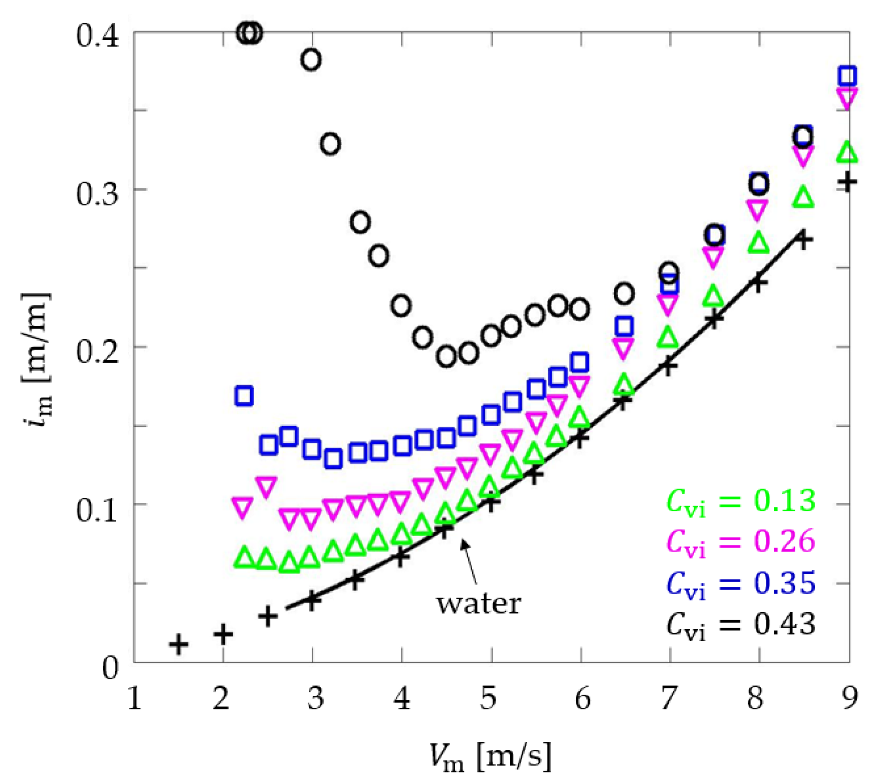
A two-fluid model for slurry pipe flows not relying on the KTGF was proposed in Roco and Shook [153]. Its peculiar feature resides in the introduction of a “supported load” concept, which is defined as the weight of that fraction of solid particles that, for each layer of a horizontal pipe flow, is supported through Coulombic contact with other particles or directly on the wall. The rest of the weight of the particles is supported by turbulent diffusion and dispersive stresses. Empirical closures are provided for the stresses arising from the three mechanisms, which involve submodels and a triplet of numerical coefficients. In this paper, a large experimental database was considered for calibration of the model, which covers a wide range of particle sizes (0.165 mm~13 mm), pipe diameter (50 and 500 mm), bulk fluid velocity (up to 4.33 m/s) and solid concentration (up to 40% by volume). The same set of empirical coefficients produced a good agreement with the experiments in terms of concentration and velocity profiles as soon as the ratio of particle size to pipe diameter is sufficiently small.
One year later, the model was extended to an arbitrary number of dispersed phases [154]. The new formulation did not increase the type and number of sub-models and coefficients, and, particularly, the same settings recommended in [153] were employed for the validation in [154]. Good agreement with experimental data was obtained in terms of pressure drop, local concentration, velocity profile and particle size distribution for a non-uniformly graded coal–water slurry flow in two pipes with the diameter of 158 mm and 495 mm, suggesting a pipe size-up scalability of the model. The authors also defined the applicability limits of their approach, which was for solid concentrations up to 60–70% of the maximum packing value and particle size to pipe diameter ratio up to 1/20.
Roco and Balakrishnam [110] improved the formulation in [153] by adding a one equation turbulence model. A more comprehensive derivation of the fundamental conservation equations was carried out following a double-averaged approach, but several modelling approximations and simplifications were made to obtain the final set of equations. The number of sub-models and parameters increased compared to [153], and a re-calibration was necessary to fit the new experimental data. The calibration/validation database consisted of eight flow conditions, characteristics of fine size sand and medium-size glass beads slurries flowing in relatively small pipes (51.5 and 40 mm) at moderate concentrations (0.10 to 0.20). The comparison with the experiments was reported for two cases only, and was performed by referring to the velocity and concentration maps over a pipe section. Using the calibrated model, the influence exerted by the inclination of pipe on mixture velocity and relative velocity distribution was investigated.
Roco and Mahadevan [155,156] continued this research line by incorporating a new turbulence model in the same framework, and provided some comparison with experimental data for single- and multi-species slurry flows. One interesting feature of this paper is that the authors provided some discussion around the appropriate wall boundary conditions, mentioning that a “modified log law” was adopted under the assumption that the particle size is small compared with the boundary layer thickness. Additionally, they also verified that about 40 pipe diameters are required to obtain a fully developed flow from the inlet conditions, which, in their setup, were uniform in terms of concentration but not in terms of velocity.
The studies of Roco and co-workers represented important achievements in the CFD modelling of slurry transport in pipes, even more so because they were obtained in a period when commercial CFD codes were not so common and the capabilities of computers were far from today standard. The two-fluid models were implemented in in-house codes, and specific strategies were developed to numerical solve the equations, some of which exploited specific features of the horizontal pipe geometry. Indeed, the supported load concept is a smart approach to account for the Coulombic contacts in the system, but, at the same time, it is difficult to generalize to other geometries than horizontal pipes. This certainly represents a significant limitation of the model, which might partially explain the lack of any follow-up. Conversely, a strength of the research work resides in the clear identification of submodels and coefficients, and in the fact that the extensive comparison against experimental data over a wide range of flow conditions, which gives confidence in the predictive capacity of the model.

4.5.2. The β - σ Two-Fluid Model for Fully Suspended Flow

About thirty years later, one of the authors of this paper and other co-workers developed a two-fluid model for the simulation of slurry pipe flows which does not employ constitutive equations from the KTGF but relies on empirical closures. The model was built by complementing the IPSA of Spalding [157], embedded in the PHOENICS code, with a number of user-defined functions. The formulation of the IPSA resembles that of a double-averaged two-fluid model in which all variables are the time-averaged of the volume-averaged quantities. Therefore, phase diffusion terms are present in all conservation equations, and they are modeled through the gradient diffusion approximation. Compared to the more general formulation in Equations (63)–(66), the IPSA involves the following main simplifications: it ignores the kinetic and collisional contributions to the pressure of the solid phase; it assumes the laminar and eddy viscosities of the solid phase to be equal to those of the liquid phase; it assumes the turbulent kinetic energy to be a property of the liquid phase. Additionally, the drag coefficient is evaluated by the correlation of Clift et al. [78] for spherical particles, and a zero wall shear stress boundary condition to the solid phase. All these approximations and simplifications appear reasonable for dilute flows, but they produce inaccurate predictions in the case of slurry pipe transport at moderate and high solid loading.
In order to overcome this limitation, in the first stage of their research, Messa et al. [37] applied two modifications to the IPSA. Firstly, they evaluated the particle Reynolds number in the drag coefficient correlation in terms of a friction-related parameter, μ m . This parameter, in turn, was obtained from an algebraic correlation analogous to the formula of Moody for the rheology of colloidal liquid–solid suspensions [104]. Thus, μ m is an increasing function of the local solid volume fraction, and it also depends on two empirical coefficients, called [ η ] and α pm , both treated as calibration parameters. Defining the particle Reynolds with respect to μ m instead of the viscosity of the pure liquid allows accounting for the increased flow resistance encountered by a particle in a slurry mixture. The second modification to the IPSA was the application of a wall function to the solid phase in order to model the influence of the solids on the wall shear stress. This was obtained by forcing the execution of a built-in PHOENICS subroutine, which, by default, is employed only for the liquid phase. Messa et al. [37] analyzed the influence of the numerical sources of uncertainty and, particularly, they found that the predicted hydraulic gradient was significantly influenced by the value of y + (Figure 19a). For slurry flows in horizontal pipes, the definition of y + is not as straightforward as in single-phase flows, and, in the works by Messa and co-workers, y + was calculated as the average over all near-wall cells in the region of fully-developed flow and expressed as a function of the friction velocity of the liquid phase. Based on these findings, the authors recommended defining the size of the near-wall cells such that y + = 30, as this is the smallest possible value consistent with the application of the wall function for the liquid phase. An experimental database covering a relatively large range of particle sizes (0.09 mm to 0.52 mm), pipe diameter (50 to 150 mm), bulk fluid velocity (up to 7 m/s) and solid concentration (up to 40% by volume), was employed for calibration and validation of the model. The same values of the calibration coefficients [ η ] = 2.5 and α pm = 0.7 (to which the turbulent Schmidt number for volume fractions in the phase diffusion terms, σ = 0.7, shall be added) procured good agreement with the experimental data for hydraulic gradient, concentration profile, and velocity profile provided that the no particle accumulation occurs. Particularly, the deviation between predicted and measured hydraulic gradient was found to lie in the range [−20%, 20%], and it is reduced if the particles are sufficiently small. This condition was identified by d p + < 50 , being d p + the particle size in wall units.
One year later, Messa and Malavasi [72] improved their model by making three changes. Firstly, they did not take the viscosity of the solid phase equal to that of the liquid phase, as in the original IPSA, but they evaluated μ s from the friction-related parameter μ m through Equation (31). Secondly, they changed the expression for μ m from the Moody-like formula to the exponential correlation of Cheng and Law [53]:
μ m = μ l exp { 2.5 β [ 1 ( 1 Φ s ) β 1 ] }
Like Moody’s, the formula of Cheng and Law was also developed for the evaluation of the viscosity of suspensions of small particles in a liquid, and here was employed for the friction-related parameter μ m which, in spite of the same symbol, has a different physical meaning. Additionally, Equation (98) involves only a single numerical coefficient, β , which Messa and Malavasi [72] argued to depend on the shape of the particles ( β = 1.5 for glass beads; β = 3.0 for regular sand; β ≈ 3.3 for highly sharp sand). The last improvement made to the two-fluid model consists in the wall boundary condition of the solid phase. Instead of forcing the execution of a built-in PHOENICS subroutine for the liquid phase, a user-defined wall function was developed and implemented in the code, which consists of a blending of a log-law like function for d p + < 30 and an empirical expression for d p + > 50 . The new formulation of the model not only decreased the number of calibration coefficients from three ( [ η ] , α pm , σ ) to two ( β and σ ), but it also allowed extending the applicability to larger particle sizes. After setting σ = 0.7 and deciding the value of β from the gross shape of the grains, good predictive capacity was obtained in terms of hydraulic gradient (deviation within [−10%, 10%]), concentration profile and velocity profile. The experimental database was larger than that in the earlier works, in terms of particle sizes (0.09 mm to 0.64 mm), pipe diameter (50 to 200 mm), bulk fluid velocity (up to 9 m/s) and solid concentration (up to 0.40 by volume).
Messa and Matoušek [57] provided the most throughout assessment of the capability of the two-fluid model presented in [72], the only difference being that the wall function of the solid phase was restricted to the log-law like branch, valid up to d p + = 30 . Particularly, the authors assessed that β is not only a function of the shape of the particles, but of the testing conditions in a broad sense. They introduced the name β - σ two fluid model to highlight the existence of two main calibration parameters, and proposed guidelines for their calibration. In addition to the “modelling” features, a significant part of the work was devoted to investigating the role played by “numerical” features. These include the length of the domain needed to attain fully developed flow from a uniform inlet, which was found to be around 100 pipe diameters, and the effect of the grid. In relation to this aspect, the predicted hydraulic gradient was found substantially insensitive to the near-wall mesh resolution (quantified by the area-averaged y + in the fully-developed region), in apparent contrast with the findings in Messa et al. [37]. Another added value of the paper [57] is that, for the first time, the concepts of interpretative and predictive models are explicitly introduced for slurry pipe flow simulations. On the one hand, it was shown that, after calibrating β and σ from hydraulic gradient data and concentration profiles, the two-fluid model could be used to get information on difficult-to-measure yet engineering-relevant features of the flow for the same flow conditions, such as the wall shear stresses distribution or the local velocity field. On the other, the predictive value of the β - σ two fluid model was subject of discussion by preliminary addressing the problem of pipe size up scalability, that is, by showing that the values of β and σ obtained from calibration at the laboratory scale are suitable to simulate flows of the same slurry mixture in bigger pipes. As a necessary prerequisite of predictive models, the applicability conditions of the β - σ two fluid model were clearly defined in terms of three conditions which could be easily verified a priori.
The latest publication on the β - σ two-fluid model is Messa et al. [38], which, as already mentioned in Section 1.3, introduced the idea of justifying the numerical solution of a CFD model in the light of its mathematical structure as a preliminary step before addressing the problem of assessing its physical consistency. Although the work is mainly focused on slurry flows in large channels, modeled as 2D, it also addresses the circular pipe case. Particularly, it sheds a light on the effect of y + on the predicted hydraulic gradient, resolving the apparent contradiction between the findings in Messa et al. [37] (preliminary version of the model, in which the built-in PHOENICS subroutine for the liquid phase was enforced to the solid one) and Messa and Matoušek [57] (the final version of the model, in which a user-defined wall function was implemented). Note that the model used in Messa et al. [38] is the same as in Messa and Matoušek [57]. The results in Figure 19b indicate that, even with the final version of the model, i m might be affected by y + , although the trend is less pronounced and qualitatively different from that obtained with the preliminary formulation (Figure 19a). However, the effect of y + on i m appears significant only at high solid volume fractions (black line in Figure 19b). In Messa and Matoušek [57], the sensitivity analysis of i m upon y + was performed only for a test case with 0.10 volumetric concentration, and this might explain why no influence of y + was detected. Based on the more general findings in Figure 19b, it was still recommended to fulfill the constraint y + = 30.
In summary, the main strength of the β - σ two-fluid model resides in the extensive work made to identify the empirical coefficients and assess their role on different features of the solution. Additionally, the studies of Messa and co-workers showed that, under certain conditions, employing closures from the KTGF is unnecessary to simulate slurry pipe flows, and that a simple model like the β - σ one can provide reliable predictions. Finally, relying on the well-established IPSA solver makes the β - σ two-fluid model computationally efficient, numerically robust, and easy to converge; actually, using the parabolic IPSA solver embedded in PHOENICS, an approximation solution for a straight pipe flow can be obtained in a few minutes on a standard computer, and this opens up the possibility of running massive sensitivity analyses. At the same time, there are still several limitations that deserve further research. Firstly, the relatively limited range of applicability of the β - σ two-fluid model precludes the possibility to simulate flows in the heterogeneous regime, which are very relevant for the applications. Secondly, the two main coefficients β and σ are not well characterized, even if attempts were made to associate their effects to specific features of the flow.

4.6. Studies Using the Mixture Model

Contributions found in the literature for applications of the Mixture Model, in conjunction with either the standard or RNG k - ε turbulence model, have been mostly focused on horizontal turbulent flow in circular pipes. As already shown in Figure 15b, studies based on the Mixture Model are a relatively limited part of the amount of published literature on slurry pipe flows. This might be explained by several reasons, including the fact that, if the interest is on monodisperse slurries, running a full Eulerian–Eulerian simulation is now completely affordable even on standard computers. In these publications, the Mixture Model was used to numerical describe mostly pressure drop, velocity and solids distribution profiles in the pipe cross section with water as the continuous fluid and several concentrations of settling particles, either silica/glass or zircon particles, ranging from dilute to concentrated, acting as the dispersed phase [67,158,159,160].
Two authors of this paper also applied the Mixture Model to describe the horizontal pipe flow of a mixture of water and glass beads/spheres with two different average particle sizes, 0.15 and 0.5 mm, and increasing volumetric concentration up until 0.11 (v/v) [161,162]. For lower flow rates and higher particle concentrations, a moving bed was formed and the pressure gradient was underpredicted which was not unexpected since this is a known limitation of the Mixture Model as documented in the literature [158].
This known limitation of the Mixture Model has been the subject of some recent studies where a numerical expression for the slip velocity between phases has been introduced as an alternative to Equation (74) for the computation of the sediment motion in both steady and unsteady open-channel flows, as well as in oscillatory flows [163]:
U V = τ p Φ l   ρ l ρ m   ( P + S )
where τ p is the response time of a particle in the mixture, and P and S are vectors accounting for the effect of pressure and the viscous stresses on the relative velocity. The open channel flow simulations in [163] do not solve for the free surface flow, but involve a fixed domain with a top boundary rigid lid with free slip is usually considered with the sediment requiring to satisfy the zero flux condition in that region.
Pipe erosion and deposition of particles in bends are also subjects of industrial significance where the Mixture Model has been used interpretably. Numerical studies can be found in the literature quantifying the effect of bend and flow velocities on the deposition of particles in a horizontal test loop [164] and on the benefits of using the Mixture Model on suspension flows through bend geometries, with and without upstream swirl induction in commercial pipelines to optimize and reduce wear by reducing particle impingements over the entire inner surfaces of a bend [165,166]
Another field of study where the Mixture Model has been used to numerically describe the flow characteristics are cryogenic slurry flows of hydrogen. Owing to the intrinsic difficulty in conducting experimental investigations at cryogenic conditions numerical simulations serve to explore and optimize hydrogen transportation. One such example is the application of a three-dimensional two-phase mixture model, coupled with k-ε mixture turbulence model, in the optimization of hydrogen loading and transportation of a helium–hydrogen slurry in cuboidal channels [167].
Additionally, the mixture model has been used not only to describe fully developed solid/liquid flows but also to describe the entrance region of a slurry flow in a horizontal pipe (up to a length equal to 50 pipe diameters), calculating the developing processes of volume fractions and density distribution of particles, mean velocity profiles and mean skin coefficient distribution [159]. A simplified 3D algebraic slip mixture model (algebraic relation for the relative velocity) was used. The model was applied to single and double species slurry flows in different flow regimes: pseudo-homogeneous, heterogeneous or heterogeneous with sliding bed. Some trends could be identified in the entrance region when varying the type of particles and the flow velocity. Additionally, trends regarding the evolution as the distance from entrance increases are coherent with what was to be expected and with the results for the fully developed region.
Finally, the Mixture Model has recently been coupled with more complex turbulence models such as the LES (Large Eddy Simulation) WALE model [168]. In this study, the numerical description of transport of unsteady sediment–water mixtures, with different particle diameters, in an open channel (tilting flume) is shown to be able to match experimental data with a high degree of accuracy for low and high particle concentrations, but with a less favorable agreement for intermediate particle concentrations. Note that, as in [163], the open channel flow was simulated by prescribing a fixed, flat top boundary, where a free slip condition is applied.
One of the important features when applying the Mixture model to slurry flows in pipes and channels is the adequate modelling of the wall region. As already mentioned in Section 2.3.3, in general, the no-slip velocity at the wall is coupled either with an algebraic variation of velocity of the mixture near the wall or with an empirical correlation to describe that variation. For instance, the Lauder and Spalding wall function [67,158,159] or the standard Fluent wall function, based on the properties of the mixture, have been used. In [163], a slightly different formulation of the log law is imposed.
In general, the Mixture Model is a low computational effort model that has proved adequate to describe both the flow of settling and buoyant solid/liquid suspensions in different geometries, showing good performance for both low to intermediate concentrations and intermediate to high velocities, as described above. The model fails to predict the required flow parameters once a bed of particles forms at the bottom of the pipe. So far, the model has mainly been used as an interpretive model but the studies presented in the literature show its capability to be used in the future as a predictive model which will favor application at the industrial level.

5. Concluding Remarks and Recommendations

This review paper shows that Computational Fluid Dynamics have great potential for application to slurry flows in pipelines, not only in the context of academic research but also for advanced pipeline design and management. CFD, in fact, can complement the traditional methods based on laboratory experiments and simplified theoretical modelling, which suffer from size constraints and cannot provide detailed information at the local scale. The increased capability of computer power, accompanied by a widespread diffusion of multi-purpose codes, makes CFD accessible to a wide community nowadays. Nonetheless, the reader will be now aware that achieving reliable CFD results is not as straightforward as it might appear at first glance. Firstly, the user must clearly establish whether the scope of the simulation is to provide insight into difficult-to-measure quantities for the same flow conditions used to calibrate the model (interpretative purpose) or, rather, to achieve quantitative information for other flow conditions (predictive purpose). Bearing this in mind, the user must complete all the necessary steps to provide confidence to the solution, and this requires mastering the concepts of numerical convergence, calibration, validation, sensitivity on submodels and coefficients, etc. This, clearly, creates challenges for the CFD side, but also for the experimental one. High-quality experimental data are needed to properly calibrate and validate a CFD model, and, focusing on the specific application of slurry pipe flows, this requires measuring other variables rather than the traditional ones (hydraulic gradient and mean concentration profile), as well as testing large diameter pipes.
Coming back to the CFD modelling side, a summary of the key modelling approaches, including the main application field, as well as the main strengths and limitations, are summarized in Table 1, and they will be discussed hereafter.
It appears that CFD-DEM models accounting for particle–particle interactions provide a lot of information, so they appear a suitable approach when deep insight into the particle-laden flow is needed at the particle and sub-particle scale for different flow patterns (mainly heterogeneous and stratified flow). However, these models are still computationally too expensive to be a practically usable tool for the engineering handling of slurry pipelines, at least for the moment. In reality, the published literature is limited to a few yet valuable examples of interpretive models, mostly focused on the understanding of the physics of turbulent, particle-laden flows. Conversely, Eulerian–Lagrangian models are widely used and still appear the most effective approach for engineering slurry erosion prediction, but only for low solid concentrations when the effect of inter-particle collisions can be ignored. The main drawback of these models is not the computational cost, which is generally affordable even on standard computers, but rather the considerable dependence of the erosion estimates upon uncertain or simply difficult-to-decide submodels, parameters and coefficients, a key role being played by the erosion models used to the turn the particle–wall impact characteristics into erosion estimates.
However, the Eulerian–Eulerian approach seems the preferred one to simulate slurry flows in pipelines. Actually, this is an obvious choice, as the Eulerian description of the solid phase is the only viable way to simulate slurries with massive amounts of solids, as typically encountered in hydro-transport applications. Although Eulerian–Eulerian models do not provide any information at the particle scale, they allow for a spatially distributed characterization of the flow, thus giving deeper insight compared to experiments and integral-scale models. Most of the studies were performed using two-fluid models based on the Kinetic Theory of Granular Flows, probably also taking advantage by the fact that models of this type are nowadays embedded in most commercial CFD codes. KTGF models have a strong physical basis, and take into account the effects produced by different types of particle–particle collisions on the flow. A good match with experiments has been reported for a wide range of flow conditions and different flow patterns (mainly heterogeneous flow) even if some doubts on their capability remain for coarse particle slurries. Additionally, it should be borne in mind that uncertain modelling features come into play even in the KTGF models, in addition, of course, to the usual numerical features. Therefore, validation and sensitivity analyses are of utmost importance to gather confidence in the predictions, and further research is needed in this sense. Finally, it is recalled that KTGF closures are not really required to simulate accurately specific types of slurry flows. This is the case, for instance, of slurry flows in the pseudo-homogeneous regime, for which two-fluid models based on simpler empirical closures proved to be not only reliable, but also predictive in a well-defined applicability range. As a concluding remark, the potential of multi-fluid models to simulate broadly graded slurry mixtures in the Eulerian framework seems overcome by the high mathematical complexity and difficulty in achieving a stable, converged solution. Conversely, the mixture model is computationally more effective, but it relies on stringent assumptions on the slurry flow (for instance, it fails in providing an accurate solution when a bed of particles form at the pipe bottom). Nonetheless, further research is required to assess the real capability of the mixture model as either an interpretative or a predictive tool.

Author Contributions

G.V.M. conceived the outline of the paper and its structure, inviting the other co-authors to take part to the project. Sync-up online meetings of all co-authors were schedule every three-four weeks, to discuss the current state of the project and decide the next steps. All co-authors contributed to the literature review and to the final editing. In terms of paper writing, their contributions were as follows. Section 1: V.M. and G.V.M. Section 2.1: F.J.d.S. and C.A.R.D. Section 2.2: G.V.M. and Q.Y. Section 2.3: G.V.M. Section 3: G.V.M. Section 4.1: G.V.M. Section 4.2: Z.C. Section 4.3: F.J.d.S. and C.A.R.D. Section 4.4: R.S.S. and O.E.A. Section 4.5: Q.Y. and G.V.M. Section 4.6: M.G.R. and R.C.S. Section 5: G.V.M. All authors have read and agreed to the published version of the manuscript.

Funding

The research at CIEPQPF, University of Coimbra was supported by the Strategic Research Centre Project UIDB00102/2020, funded by FCT, Portugal. The research at Institute of Hydrodynamics of Czech Academy of Sciences was supported by the Czech Science Foundation through the grant project No. 20-13142S.

Conflicts of Interest

The authors declare no conflict of interest.

Nomenclature

SymbolUnitsDescription
C d -drag coefficient
C ls kg/(m3 s)fluid–solid exchange coefficient
C vd -delivered solids concentration
C vi -average spatial volumetric concentration of solids
d p mparticle diameter
d p + -particle size in wall units
Dmpipe diameter
D ls kg/(m3 s)fluid–solid exchange coefficient
e n -
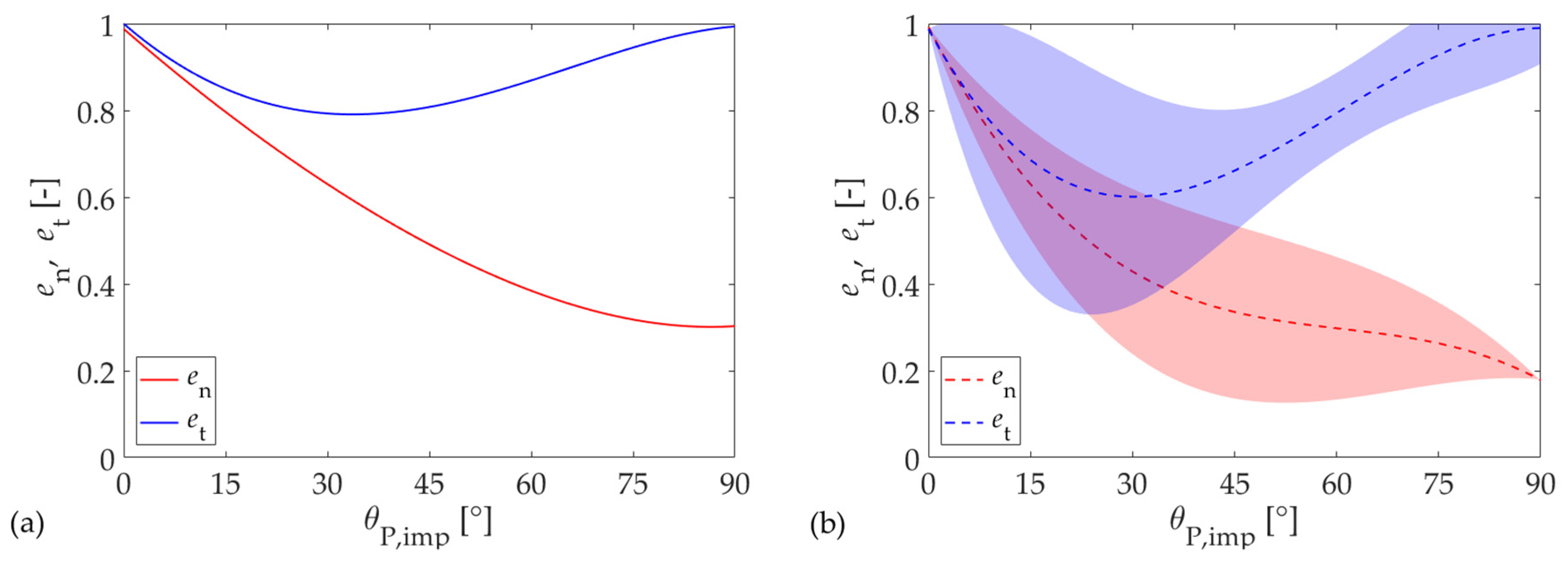
normal particle(parcel)-wall restitution coefficients
e ss -inter-particle collision restitution coefficient
e t -tangential particle(parcel)-wall restitution coefficients
F -dimensionless wear function in Equation (81)
F s -particle shape related constant in Equation (86)
g 0 , ss -radial distribution function
i m -hydraulic gradient
I 2 D Pa2second invariant of the deviatoric stress tensor
I p kg m2moment of inertia of the particle
km2/s2turbulent kinetic energy
k Θ s -diffusion coefficient in Equation (88)
K -material related constant in Equation (86)
K ls kg/(m3 s)fluid–solid exchange coefficient
mkgmass of a particle
N p -number of particles in the sampling volume W
Rep-particle Reynolds number
pPainstantaneous pressure
p ˜ s , coll Pacollisional solid pressure
p ˜ s , fric Pafrictional solid pressure
p ˜ s , kin Pakinetic solid pressure
PPalocally-averaged/double-averaged pressure
P k l m2/s3volumetric production rate of k l
n d -number of particle size classes
n -velocity exponent in Equation (86)
Q m3/svolumetric flow rate
S p -relative density of particle
tstime
T stime scale
v imp m/smodulus of the impact velocity
V dl m/sdeposition-limit velocity
V m m/sslurry bulk-mean velocity
Wm3sampling volume
y+-dimensionless distance of the first grid point to the wall
Vectors and tensors
F D Ndrag force
F p Nforces exerted on the particle
f ˜ l s Ntotal force from liquid to solid phase in sampling volume
g m/s2gravitational acceleration vector
m N/m3momentum exchange term in Eulerian–Eulerian formulation
m d N/m3generalized drag in the Eulerian–Eulerian formulation
m ˜ ¯ td N/m3turbulent dispersion force
P m/s2pressure-related vector in Equation (97)
S m/s2viscosity-related vector in Equation (97)
S l N/m3momentum exchange term in Eulerian–Lagrangian framework
T p N mtorque exerted on the particle
u m/sinstantaneous velocity vector of the liquid phase
u , u m/sfluctuating velocity vector of the liquid phase
U ls 0 m/sthe solution of Equation (73) without the last term
U mk m/sdiffusion velocities in mixture model
v m/sinstantaneous velocity vector of a particle/solid phase
v and v m/sfluctuating velocity vector of the solid phase
x mposition vector
σ Pastresses tensor
σ pt , k Papseudo-turbulent stress tensors
τ Padeviatoric part of the stresses tensor
τ m t Pa“Reynolds”-like stresses in the mixture model
τ Dm Padiffusion stresses in the mixture model
ω p s−1angular velocity vector of the particle
Greek Symbols
α pm -empirical coefficient in two-fluid model of Messa et al. [37]
β -numerical coefficient in   β -σ two fluid model
γ s kg/(m3 s)rate of energy dissipation due to collision within the solid particles
εm2/s3turbulence dissipation rate
η merosion depth
[ η ] -empirical coefficient in two-fluid model of Messa et al. [37]
θ °angle of internal friction of particle
θ imp °impact angle
Θ s m2/s2granular temperature
λ Pa ssecond viscosity coefficient or bulk viscosity
μ Pa sdynamic viscosity
μ eff Pa seffective viscosity
μ t Pa seddy viscosity
μ s , coll Pa scollisional solid viscosity
μ s , fr Pa sfrictional solid viscosity
μ s , kin Pa skinetic solid viscosity
ρ kg/m3density
σ -turbulent Schmidt number for volume fractions
τ p sresponse time of a particle in the mixture
φ -particle spherical coefficient
φ ls kg/(m3 s) exchange term in Equation (88)
Φ e kg/(m2 s)erosion rate intensity
Φ m kg/(m2 s)local average particle impact rate
Φ -instantaneous volume fraction of one phase
Φ -fluctuating volume fraction of one phase
ω s−1specific turbulent dissipation rate
Subscripts and superscripts
beforejust before a particle–wall impact occurs
afterjust after a particle–wall impact has occurred
iinterface
kgeneric phase
lliquid phase
mmixture
pphysical particles
Pcomputational particles in the Lagrangian framework
ssolid phase in the Eulerian framework
ttarget material in erosion modelling
@pat particle position in Eulerian–Lagrangian modelling
@Pat parcel position in Eulerian–Lagrangian modelling
normal to the wall
parallel to the wall
Operators (applied to the generic variable ψ)
+transpose of a tensor
ψ ˜ volume-average
ψ ¯ time-average
ψ Favre-average
Ψ generic averaged (or double averaged) variable
Acronyms
CFDComputational Fluid Dynamics
DDPMDense Discrete Particle Model
DEMDiscrete Element Method
DNSDirect Numerical Simulation
ELEulerian–Lagrangian model (or approach)
GCIGrid Convergence Index
IPSAInter-Phase Slip Algorithm
KTGFKinetic Theory of Granular Flow
LESLarge Eddy Simulation
RANSReynolds-Averaged Navier–Stokes
RSMReynolds Stress Model
SECSpecific Energy Consumption
U-RANSV-Unsteady Reynolds-Averaged Navier–Stokes

References

  1. Derammelaere, R.H.; Shou, G. Altamina’s Copper and Zinc Concentrate pipeline incorporates advanced technologies. In Proceedings of the 15th International Conference on Hydrotransport, Banff, AB, Canada, 3–5 June 2002. [Google Scholar]
  2. Paterson, A.J.C. Pipeline transport of high density slurries: A historical review of past mistakes, lessons learned and current technologies. Min. Technol. 2012, 121, 37–45. [Google Scholar] [CrossRef]
  3. van den Berg, C.H. IHC Merwede Handbook for Centrifugal Pumps and Slurry Transportation; MTI Holland: Kinderdijk, The Netherlands, 2013. [Google Scholar]
  4. van Wijk, J.M.; Talmon, A.M.; van Rhee, C. Stability of vertical hydraulic transport processes for deep ocean mining: An experimental study. Ocean Eng. 2016, 125, 203–213. [Google Scholar] [CrossRef]
  5. Thomas, A.D.; Cowper, N.T. The design of slurry pipelines—Historical aspects. In Proceedings of the 20th International Conference on Hydrotransport, Melbourne, Australia, 3–5 May 2017. [Google Scholar]
  6. Matoušek, V. Pressure drops and flow patterns in sand-mixture pipes. Exp. Therm. Fluid Sci. 2002, 26, 693–702. [Google Scholar] [CrossRef]
  7. Talmon, A.M. Analytical model for pipe wall friction of pseudo-homogenous sand slurries. Part. Sci. Technol. 2013, 31, 264–270. [Google Scholar] [CrossRef]
  8. Spelay, R.; Gillies, R.G.; Hashemi, S.A. Kinematic friction of concentrated suspensions of neutrally buoyant coarse particles. In Proceedings of the 20th International Conference on Hydrotransport, Melbourne, Australia, 3–5 May 2017. [Google Scholar]
  9. Wilson, K.C. Deposition-limit nomograms for particles of various densities in pipeline flow. In Proceedings of the 6th International Conference on Hydraulic Transport of Solids in Pipes, Canterbury, UK, 26–28 September 1979. [Google Scholar]
  10. Sanders, R.S.; Sun, R.; Gillies, R.G.; McKibbem, M.J.; Litzenberger, C.; Shook, C.A. Deposition velocities for particles of intermediate size in turbulent flow. In Proceedings of the 16th International Conference on Hydrotransport, Santiago, Chile, 26–28 April 2004. [Google Scholar]
  11. Hashemi, S.A.; Wilson, K.C.; Sanders, R.S. Specific Energy Consumption and optimum operating condition for coarse-particle slurries. Powder Technol. 2014, 262, 183–187. [Google Scholar] [CrossRef]
  12. Matoušek, V. Non-stratified flow of sand-water slurries. In Proceedings of the 15th International Conference on Hydrotransport, Banff, AB, Canada, 3–5 June 2002. [Google Scholar]
  13. Gillies, R.G.; Shook, C.A. Concentration distributions of sand slurries in horizontal pipe flow. Part. Sci. Technol. 1994, 12, 45–69. [Google Scholar] [CrossRef]
  14. Wilson, K.C.; Addie, G.R.; Sellgren, A.; Clift, R. Slurry Transport Using Centrifugal Pumps, 3rd ed.; Springer: New York, NY, USA, 2006. [Google Scholar]
  15. Shook, C.A.; Gillies, R.G.; Sanders, R.S.; Spelay, R.B. Saskatchewan Research Council Course Notes; SRC Publications: Saskatoon, SK, Canada, 2013. [Google Scholar]
  16. Durand, R. Basic Relationships of the transportation of solids in pipes—Experimental research. In Proceedings of the IAHR Minnesota International Hydraulic Convention, Minneapolis, MI, USA, 1–4 September 1953. [Google Scholar]
  17. Matoušek, V.; Visintainer, R.; Furlan, J.; Sellgren, A. Pipe-size scale-up of frictional head loss in settling-slurry flows using predictive models: Experimental validation. In Proceedings of the ASME FEDSM2020, Orlando, FL, USA, 13–15 July 2020. [Google Scholar]
  18. Wilson, K.C. A Unified physically-based analysis of solid-liquid pipeline flow. In Proceedings of the 4th International Conference on Hydrotransport, Banff, AB, Canada, 18–21 May 1976. [Google Scholar]
  19. Gillies, R.G.; Shook, C.A.; Wilson, K.C. An improved two layer model for horizontal slurry pipeline flow. Can. J. Chem. Eng. 1991, 69, 173–178. [Google Scholar] [CrossRef]
  20. Doron, P.; Barnea, D. A three-layer model for solid-liquid flow in horizontal pipes. Int. J. Multiph. Flow 1993, 19, 1029–1043. [Google Scholar] [CrossRef]
  21. Gillies, R.G.; Shook, C.A. Modelling high concentration slurry flows. Can. J. Chem. Eng. 2000, 78, 709–716. [Google Scholar] [CrossRef]
  22. Gillies, R.G.; Shook, C.A.; Xu, J. Modelling heterogeneous slurry flows at high velocities. Can. J. Chem. Eng. 2004, 82, 1060–1065. [Google Scholar] [CrossRef]
  23. Spelay, R.B.; Hashemi, S.A.; Gillies, R.G.; Hegde, R.; Sanders, R.S.; Gillies, R.G. Governing friction loss mechanisms and the importance of off-line characterization test in the pipeline transport of dense coarse-particle slurries. In Proceedings of the ASME 2013 Fluids Engineering Division Summer Meeting, Incline Village, NE, USA, 7–11 July 2013. [Google Scholar]
  24. Matoušek, V.; Krupička, J. Unified model for coarse-slurry flow with stationary and sliding Bed. In Proceedings of the 15th International Conference on Transport and Sedimentation of Solid Particles, Wroclaw, Poland, 22–25 September 2015. [Google Scholar]
  25. Matoušek, V.; Krupička, J.; Kesely, M. A layered model for inclined pipe flow of settling slurry. Powder Technol. 2018, 333, 317–326. [Google Scholar] [CrossRef]
  26. Visintainer, R.; Furlan, J.; McCall, G.; Sellgren, A.; Matoušek, V. Comprehensive loop testing of a broadly graded (4-component) slurry. In Proceedings of the 20th International Conference on Hydrotransport, Melbourne, Australia, 3–5 May 2017. [Google Scholar]
  27. Matoušek, V.; Visintainer, R.; Furlan, J.; Sellgren, A. Frictional head loss of various bimodal settling slurry flows in pipe. In Proceedings of the ASME-JSME-KSME 2019 Joint Fluids Engineering Conference AJKFLUIDS 2019, San Francisco, CA, USA, 28 July–1 August 2019. [Google Scholar]
  28. Loth, E. Particle, Drops, and Bubbles. Fluid Dynamics and Numerical Methods; Draft for Cambridge University Press: 2010. Available online: www.academia.edu (accessed on 31 August 2021).
  29. Elghobashi, S. On predicting particle-laden turbulent flows. Appl. Sci. Res. 1994, 52, 309–329. [Google Scholar] [CrossRef]
  30. Sommerfeld, M. Numerical methods for dispersed multiphase flows. In Particles in Flows; Bodnár, T., Galdi, G., Nečasová, Š., Eds.; Birkhäuser: Cham, Switzerland, 2017; pp. 327–396. [Google Scholar]
  31. Leguizamón, S.; Jahanbakhsh, E.; Martens, A.; Alimirzazadeh, S.; Avellan, F. A multiscale model for sediment impact erosion simulation using the finite volume particle method. Wear 2017, 392–393, 202–212. [Google Scholar] [CrossRef]
  32. Crowe, C.T.; Troutt, T.R.; Chung, J.N. Numerical models for two-phase turbulent flows. Annu. Rev. Fluid Mech. 1996, 28, 11–43. [Google Scholar] [CrossRef]
  33. van Wachem, B.G.M.; Almstedt, A.E. Methods for multiphase computational fluid dynamics. Chem. Eng. J. 2003, 96, 81–98. [Google Scholar] [CrossRef]
  34. Hiltunen, K.; Jäsberg, A.; Kallio, S.; Karema, H.; Kataja, M.; Koponen, A.; Manninen, M.; Taivassalo, V. Multiphase Flow Dynamics. Theory and Numerics; VTT Technical Research Centre of Finland: Espoo, Finland, 2009. [Google Scholar]
  35. Manninen, M.; Taivassalo, V.; Kallio, S. On the Mixture Model for Multiphase Flow; VTT Technical Research Centre of Finland: Espoo, Finland, 1996. [Google Scholar]
  36. Ekambara, K.; Sanders, R.S.; Nandakumar, K.; Masliyah, J.H. Hydrodynamic simulation of horizontal slurry pipeline flow using ANSYS-CFX. Ind. Eng. Chem. Res. 2009, 48, 8159–8171. [Google Scholar] [CrossRef]
  37. Messa, G.V.; Malin, M.; Malavasi, S. Numerical prediction of fully-suspended slurry flow in horizontal pipes. Powder Technol. 2014, 256, 61–70. [Google Scholar] [CrossRef]
  38. Messa, G.V.; Malin, M.; Matoušek, V. Parametric study of the β-σ two-fluid model for simulating fully-suspended slurry flow: Effect of flow conditions. Meccanica 2021, 56, 1047–1077. [Google Scholar] [CrossRef]
  39. Enwald, H.; Peirano, E.; Almstedt, A.T. Eulerian two-phase flow theory applied to fluidization. Int. J. Multiph. Flow 1996, 22, 21–66. [Google Scholar] [CrossRef]
  40. Menter, F. Two equation eddy-viscosity turbulence modeling for engineering applications. AIAA J. 1994, 32, 1598–1605. [Google Scholar] [CrossRef] [Green Version]
  41. Launder, B.E.; Spalding, D.B. Mathematical Models of Turbulence; Academic Press: London, UK, 1972. [Google Scholar]
  42. Prosperetti, A.; Tryggvason, G. Computational Methods for Multiphase Flow; Cambridge University Press: New York, NY, USA, 2007. [Google Scholar]
  43. Gosman, A.D.; Ioannides, E. Aspects of computer simulation of liquid-fueled combustors. J. Energy 1983, 7, 482–490. [Google Scholar] [CrossRef]
  44. Sommerfeld, M.; Kohnen, G.; Rüger, M. Some open questions and inconsistencies of Lagrangian particle dispersion models. In Proceedings of the 9th Symposium on Turbulent Shear Flows, Kyoto, Japan, 16–18 August 1993. [Google Scholar]
  45. Hager, A. CFD-DEM on Multiple Scales. An Extensive Investigation of Particle-Fluid Interactions. Ph.D. Thesis, Johannes Kepler University Linz, Linz, Austria, 2014. [Google Scholar]
  46. Rettinger, C.; Godenschwager, C.; Eibl, S.; Preclik, T.; Schruff, T.; Frings, R. Fully resolved simulations of dune formation in riverbeds. In High Performance Computing; Kunkel, J.M., Yokota, R., Balaji, P., Keyes, D., Eds.; Springer: New York, NY, USA, 2017; pp. 3–21. [Google Scholar]
  47. Peng, Z.; Doroodchi, E.; Luo, C.; Moghtaderi, B. Influence of void fraction calculation on fidelity of CFD-DEM simulation of gas-solid bubbling fluidized beds. AIChE J. 2014, 60, 2000–2018. [Google Scholar] [CrossRef]
  48. Zheng, E.; Rudman, M.; Kuang, S.; Chryss, A. Turbulent coarse-particle suspension flow: Measurement and modelling. Powder Technol. 2020, 373, 647–659. [Google Scholar] [CrossRef]
  49. Launder, B.E.; Spalding, D.B. The numerical computation of turbulent flows. Comput. Meth. Appl. Mech. Eng. 1974, 3, 269–289. [Google Scholar] [CrossRef]
  50. Huber, N.; Sommerfeld, M. Modelling and numerical calculation of dilute-phase pneumatic conveying in pipe systems. Powder Technol. 1998, 99, 90–101. [Google Scholar] [CrossRef]
  51. Breuer, M.; Alletto, M.; Langfeldt, F. Sandgrain roughness model for rough walls within Eulerian-Lagrangian predictions of turbulent flows. Int. J. Multiph. Flow 2012, 43, 157–175. [Google Scholar] [CrossRef]
  52. Messa, G.V.; Wang, Y. Importance of accounting for finite particle size in CFD-based erosion prediction. In Proceedings of the ASME 2018 Pressure Vessels and Piping Conference, Prague, Czech Republic, 15–20 July 2018. [Google Scholar]
  53. Cheng, N.S.; Law, A.W.K. Exponential formula for computing effective viscosity. Powder Technol. 2003, 129, 156–160. [Google Scholar] [CrossRef]
  54. Gomex, L.C.; Milioli, F.E. Collisional solid’s pressure impact on numerical results from a traditional two-fluid model. Powder Technol. 2005, 149, 78–83. [Google Scholar]
  55. Burns, A.D.; Frank, T.; Hamill, I.; Shi, J.M. The Favre averaged drag model for turbulent dispersion in Eulerian multi-phase flows. In Proceedings of the 5th International Conference on Multiphase Flow, Yokohama, Japan, 30 May–4 June 2004. [Google Scholar]
  56. Spalding, D.B. PHOENICS Encyclopedia. Models for Two-Phase Flows: Two-Equation k-ε Turbulence Model. Available online: http://www.cham.co.uk/phoenics/d_polis/d_enc/turmod/enc_tu74.htm (accessed on 22 July 2021).
  57. Messa, G.V.; Matoušek, V. Analysis and discussion of two fluid modelling of pipe flow of fully suspended slurry. Powder Technol. 2020, 30, 747–768. [Google Scholar] [CrossRef]
  58. Elghobashi, S.E.; Abou-Arab, T.W. A two-equation turbulence model for two-phase flows. Phys. Fluids 1983, 26, 931–938. [Google Scholar] [CrossRef]
  59. Crowe, C.T. On models for turbulence modulation in fluid-particle flows. Int. J. Multiph. Flow 2000, 26, 719–727. [Google Scholar] [CrossRef]
  60. Chen, P.E.; Wood, C.E. A turbulence closure model for dilute gas-particle flows. Can. J. Chem. Eng. 1985, 63, 349–360. [Google Scholar] [CrossRef]
  61. Mostafa, A.A.; Mongia, H.C. On the interaction of particles and turbulent fluid flow. Int. J. Heat Mass Transf. 1988, 31, 2066–2075. [Google Scholar] [CrossRef]
  62. Hadinoto, K.; Curtis, J.S. Effect of interstitial fluid on particle-particle interactions in kinetic theory approach of dilute turbulent fluid-particle flow. Ind. Eng. Chem. Res. 2004, 43, 3604–3615. [Google Scholar] [CrossRef]
  63. Hadinoto, K. Predicting turbulence modulation at different Reynolds numbers in dilute-phase turbulent liquid-particle flow simulations. Chem. Eng. Sci. 2010, 65, 5297–5308. [Google Scholar] [CrossRef]
  64. Hadinoto, K.; Chew, J.W. Modeling fluid-particle interaction in dilute-phase turbulent liquid-particle flow simulation. Particuology 2010, 8, 150–160. [Google Scholar] [CrossRef]
  65. Mandø, M.; Lightstone, M.F.; Rosendahl, L.; Yin, C.; Sørensen, H. Turbulence modulation in dilute particle-laden flow. Int. J. Heat Fluid Flow 2009, 30, 331–338. [Google Scholar] [CrossRef]
  66. Messa, G.V.; Malavasi, S. Numerical prediction of dispersed turbulent liquid–solid flows in vertical pipes. J. Hydraul. Res. 2014, 52, 684–692. [Google Scholar] [CrossRef]
  67. Kaushal, D.R.; Thinglas, T.; Tomita, Y.; Kuchii, S.; Tsukamoto, H. CFD modeling for pipeline flow of fine particles at high concentration. Int. J. Multiph. Flow 2012, 43, 85–100. [Google Scholar] [CrossRef]
  68. Melville, W.K.; Bray, K.N.C. A model of the two-phase turbulent jet. Int. J. Heat Mass Transf. 1979, 22, 647–656. [Google Scholar] [CrossRef]
  69. Loth, E. An Eulerian turbulent diffusion model for particles and bubbles. Int. J. Multiph. Flow 2011, 27, 1051–1063. [Google Scholar] [CrossRef]
  70. Mashayek, F.; Taulbee, D.B. A four-equation model for prediction of gas-solid turbulent flows. Num. Heat Transf. Part B 2002, 41, 95–116. [Google Scholar] [CrossRef]
  71. Johnson, P.C.; Jackson, R. Frictional-collisional constitutive relations for granular materials, with application to plane shearing. J. Fluid Mech. 1987, 176, 67–93. [Google Scholar] [CrossRef]
  72. Messa, G.V.; Malavasi, S. Improvements in the numerical prediction of fully-suspended slurry flow in horizontal pipes. Powder Technol. 2015, 270, 358–367. [Google Scholar] [CrossRef]
  73. Ferziger, J.H.; Peric, M. Computational Methods for Fluid Dynamics; Springer: Berlin/Heidelberg, Germany; New York, NY, USA, 2002. [Google Scholar]
  74. Roache, P.J. Perspective: A method for uniform reporting of grid refinement studies. ASME J. Fluids Eng. 1994, 116, 405–413. [Google Scholar] [CrossRef]
  75. Zhang, M.; Kang, Y.; Wei, W.; Li, D.; Xiong, T. CFD investigation of the flow characteristics of liquid-solid slurry in a large-diameter horizontal pipe. Part. Sci. Technol. 2020, 1–14. [Google Scholar] [CrossRef]
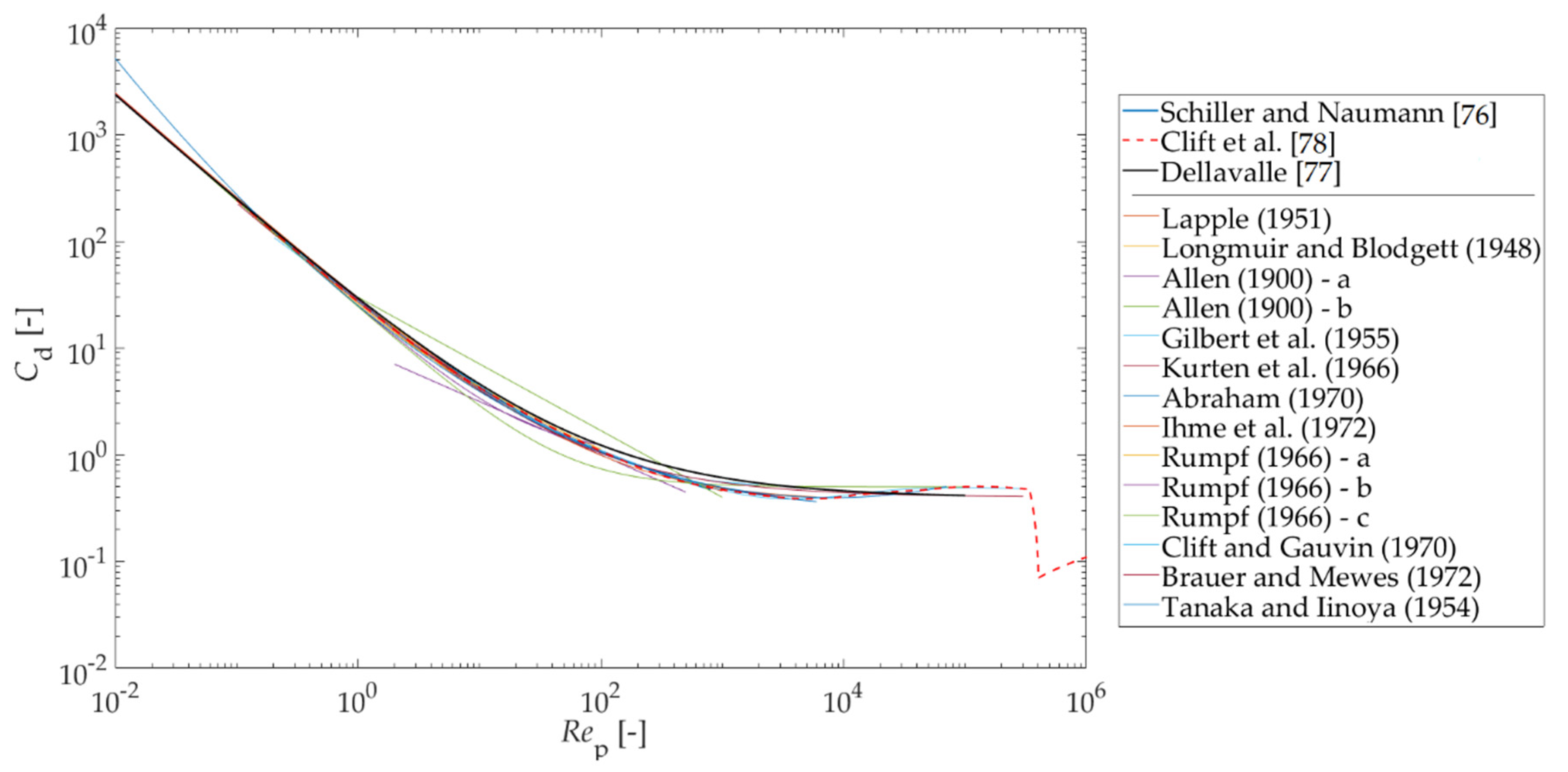
  76. Schiller, L.; Naumann, Z. A drag coefficient correlation. Z. Ver. Dtsch. Ing. 1935, 77, 318–320. [Google Scholar]
  77. Dellavalle, J.M. Micrometrics: The Technology of Fine Particles; Pitman: London, UK, 1948. [Google Scholar]
  78. Clift, R.; Grace, J.R.; Weber, M.E. Bubbles, Drops, and Particles; Academic Press: New York, NY, USA, 1978. [Google Scholar]
  79. Song, X.; Xu, Z.; Li, G.; Pang, Z.; Zhu, Z. A new model for predicting drag coefficient and settling velocity of spherical and non-spherical particle in Newtonian fluid. Powder Technnol. 2017, 321, 242–250. [Google Scholar] [CrossRef]
  80. Haider, A.; Levenspiel, O. Drag coefficient and terminal velocity of spherical and nonspherical particles. Powder Technol. 1989, 58, 63–70. [Google Scholar] [CrossRef]
  81. Yang, C.W. Handbook of Fluidization and Fluid-Particle Systems; Marcel Dekker Inc: New York, NY, USA, 2003. [Google Scholar]
  82. Forder, A.; Thew, M.; Harrison, D. A numerical investigation of solid particle erosion experienced with oilfield control valves. Wear 1998, 216, 184–193. [Google Scholar] [CrossRef]
  83. Grant, G.; Tabakoff, W. Erosion prediction in turbomachinery resulting from environmental solid particles. J. Aircraft 1975, 12, 471–478. [Google Scholar] [CrossRef]
  84. Messa, G.V.; Malavasi, S. The effect of sub-models and parameterizations in the simulation of abrasive jet impingement tests. Wear 2017, 370–371, 59–72. [Google Scholar] [CrossRef]
  85. Lyczkowski, R.W.; Bouillard, J.X. State-of-the-art review of erosion modeling in fluid/solids systems. Prog. Energy Combust. Sci. 2002, 28, 543–602. [Google Scholar] [CrossRef]
  86. Parsi, M.; Najmi, K.; Najafifard, F.; Hassani, S.; McLaury, B.S.; Shirazi, S.A. A comprehensive review of solid particle erosion modeling for oil and gas wells and pipelines applications. J. Nat. Gas Sci. Eng. 2014, 21, 850–873. [Google Scholar] [CrossRef]
  87. Oka, Y.I.; Okamura, K.; Yoshida, T. Practical estimation of erosion damage caused by solid particle impact: Part 1: Effects of impact parameters on a predictive equation. Wear 2005, 259, 95–101. [Google Scholar] [CrossRef]
  88. Oka, Y.I.; Yoshida, T. Practical estimation of erosion damage caused by solid particle impact: Part 2: Mechanical properties of materials directly associated with erosion damage. Wear 2005, 102–109. [Google Scholar] [CrossRef]
  89. Finnie, I. Erosion of surfaces by solid particles. Wear 1960, 3, 87–103. [Google Scholar] [CrossRef]
  90. Bitter, J.G.A. A study of erosion phenomena. Part I. Wear 1963, 6, 5–21. [Google Scholar] [CrossRef]
  91. Bitter, J.G.A. A study of erosion phenomena. Part II. Wear 1963, 6, 169–190. [Google Scholar] [CrossRef]
  92. Lester, D.R.; Graham, L.A.; Wu, J. High precision suspension erosion modelling. Wear 2010, 269, 449–457. [Google Scholar] [CrossRef]
  93. Mansouri, A. A Combined CFD-Experimental Method for Developing an Erosion Equation for Both Gas-Sand and Liquid-Sand Flows. Ph.D. Thesis, The University of Tulsa, Tulsa, OK, USA, 2016. [Google Scholar]
  94. Messa, G.V.; Wang, Y.; Negri, M.; Malavasi, S. An improved CFD/experimental combined methodology for the calibration of empirical erosion models. Wear 2021, 476, 203734. [Google Scholar] [CrossRef]
  95. Ishii, M.; Mishima, K. Two-fluid model and hydrodynamic constitutive relations. Nucl. Eng. Des. 1984, 82, 107–126. [Google Scholar] [CrossRef]
  96. Di Felice, R. The voidage function for fluid-particle interaction systems. Int. J. Multiph. Flow 1994, 20, 153–159. [Google Scholar] [CrossRef]
  97. Gidaspow, D. Multiphase Flow and Fluidization: Continuum and Kinetic Theory Descriptions; Academic Press: New York, NY, USA, 1994. [Google Scholar]
  98. Li, G.; Wang, Y.; He, R.; Cao, X.; Lin, C.; Meng, T. Numerical simulation of predicting and reducing solid particle erosion of solid-liquid two-phase flow in a choke. Pet. Sci. 2009, 6, 91–97. [Google Scholar] [CrossRef] [Green Version]
  99. Xu, S.L.; Sun, R.; Cai, Y.Q.; Sun, H.L. Study of sedimentation of non-cohesive particles via CFD-DEM simulations. Granul. Matter 2018, 20, 4. [Google Scholar] [CrossRef] [Green Version]
  100. Krampa-Morlu, F.M.; Bugg, J.D.; Bergstrom, D.J.; Sanders, R.S.; Schaan, J. Frictional pressure drop calculations for liquid-solid vertical flows using the two-fluid model. In Proceedings of the 14th Annual Conference of the Computational Fluid Dynamics Society of Canada, Kingston, ON, Canada, 16–18 July 2009. [Google Scholar]
  101. Messa, G.V.; Malin, M.; Malavasi, S. Numerical prediction of pressure gradient of slurry flows in horizontal pipes. In Proceedings of the ASME 2013 Pressure Vessels & Piping Division Conference, Paris, France, 14–18 July 2013. [Google Scholar]
  102. Zhao, Y.; Ding, T.; Zhu, L.; Zhong, Y. A specularity coefficient model and its application to dense particulate flow simulations. Ind. Eng. Chem. Res. 2016, 55, 1439–1448. [Google Scholar] [CrossRef]
  103. Hu, X.W.; Guo, L.J. Numerical investigations of catalyst-liquid slurry flow in the photocatalytic reactor for hydrogen production based on algebraic slip model. Int. J. Hydrogen Energy 2010, 35, 7065–7072. [Google Scholar]
  104. Mooney, M. The viscosity of a concentrated suspension of spherical particles. J. Colloid Sci. 1951, 6, 162–170. [Google Scholar] [CrossRef]
  105. Capecelatro, J.; Desjardins, O. Eulerian–Lagrangian modeling of turbulent liquid–solid slurries in horizontal pipes. Int. J. Multiph. Flow 2013, 55, 64–79. [Google Scholar] [CrossRef]
  106. Arolla, S.K.; Desjardins, O. Transport modeling of sedimenting particles in a turbulent pipe flow using Euler–Lagrange large eddy simulation. Int. J. Multiph. Flow 2015, 75, 1–11. [Google Scholar] [CrossRef] [Green Version]
  107. Uzi, A.; Levy, A. Flow characteristics of coarse particles in horizontal hydraulic conveying. Powder Technol. 2018, 326, 302–321. [Google Scholar] [CrossRef]
  108. Zhou, M.; Kuang, S.; Luo, K.; Zou, R.; Wang, S.; Yu, A. Modeling and analysis of flow regimes in hydraulic conveying of coarse particles. Powder Technol. 2020, 373, 543–554. [Google Scholar] [CrossRef]
  109. Cundall, P.A.; Strack, O.D.L. A discrete numerical model for granular assemblies. Géotechnique 1979, 29, 47–65. [Google Scholar] [CrossRef]
  110. Roco, M.; Balakrishnam, N. Multi-dimensional flow analysis of solid–liquid mixtures. J. Rheol. 1985, 29, 431–456. [Google Scholar] [CrossRef]
  111. Dahl, A.M.; Ladam, Y.; Unander, T.; Onsrud, G. SINTEF-IFE Sand transport 2001–2003. In SINTEF Internal Report; SINTEF: Trondheim, Norway, 2003. [Google Scholar]
  112. Ting, X.; Xinzhuo, Z.; Miedema, S.A.; Xiuhan, C. Study of the characteristics of the flow regimes and dynamics of coarse particles in pipeline transportation. Powder Technol. 2019, 347, 148–158. [Google Scholar] [CrossRef]
  113. Chen, Q.; Xiong, T.; Zhang, X.; Jiang, P. Study of the hydraulic transport of non-spherical particles in a pipeline based on the CFD-DEM. Eng. Appl. Comput. Fluid Mech. 2020, 14, 53–69. [Google Scholar] [CrossRef]
  114. Truscott, G.F. A literature survey on abrasive wear in hydraulic machinery. Wear 1972, 20, 29–50. [Google Scholar] [CrossRef]
  115. Duarte, C.A.R.; de Souza, F.J.; dos Santos, V.F. Numerical investigation of mass loading effects on elbow erosion. Powder Technol. 2015, 283, 593–606. [Google Scholar] [CrossRef]
  116. Duarte, C.A.R.; de Souza, F.J.; dos Santos, V.F. Mitigating elbow erosion with a vortex chamber. Powder Technol. 2016, 288, 6–25. [Google Scholar] [CrossRef]
  117. dos Santos, V.F.; de Souza, F.J.; Duarte, C.A.R. Reducing bend erosion with a twisted tape insert. Powder Technol. 2016, 301, 889–910. [Google Scholar] [CrossRef]
  118. Duarte, C.A.R.; de Souza, F.J.; de Vasconcelos Salvo, R.; dos Santos, V.F. The role of inter-particle collisions on elbow erosion. Int. J. Multiph. Flow 2017, 89, 1–22. [Google Scholar] [CrossRef]
  119. Duarte, C.A.R.; de Souza, F.J. Innovative pipe wall design to mitigate elbow erosion: A CFD analysis. Wear 2017, 380–381, 176–190. [Google Scholar] [CrossRef]
  120. Shitole, P.P.; Gawande, S.H.; Desale, G.R.; Nandre, B.D. Effect of impacting particle kinetic energy on slurry erosion wear. J. Bio-Tribo-Corros. 2015, 29, 9. [Google Scholar] [CrossRef] [Green Version]
  121. Javaheria, V.; Portera, D.; Kuokkalab, V.T. Slurry erosion of steel—Review of tests, mechanisms and materials. Wear 2018, 408–409, 248–273. [Google Scholar] [CrossRef]
  122. Messa, G.V.; Malavasi, S. A CFD-based method for slurry erosion prediction. Wear 2018, 398–399, 127–145. [Google Scholar] [CrossRef]
  123. Yu, W.; Fede, P.; Climent, E.; Sanders, S. Multi-fluid approach for the numerical prediction of wall erosion in an elbow. Powder Technol. 2019, 354, 561–583. [Google Scholar] [CrossRef] [Green Version]
  124. Zhang, J.; McLaury, B.S.; Shirazi, S.A. Application and experimental validation of a CFD based erosion prediction procedure for jet impingement geometry. Wear 2018, 394–395, 11–19. [Google Scholar] [CrossRef]
  125. Mansouri, A.; Arabnejad, H.; Shirazi, S.A.; McLaury, B.S. A combined CFD/experimental methodology for erosion prediction. Wear 2015, 332, 1090–1097. [Google Scholar] [CrossRef]
  126. Zhang, J.; Kang, J.; Fan, J.; Gao, J. Research on erosion wear of high-pressure pipes during hydraulic fracturing slurry flow. J. Loss Prevent. Proc. Ind. 2016, 43, 438–448. [Google Scholar] [CrossRef]
  127. Yang, S.; Fan, J.; Zhang, L.; Sun, B. Performance prediction of erosion in elbows for slurry flow under high internal pressure. Tribol. Int. 2021, 157, 106879. [Google Scholar] [CrossRef]
  128. Gidaspow, D.; Bezburuah, R.; Ding, J. Hydrodynamics of circulating fluidized beds: Kinetic theory approach. In Proceedings of the 7th International Conference on Fluidization, Gold Coast, Australia, 3–8 May 1992. [Google Scholar]
  129. Schaeffer, D.G. Instability in the evolution equations describing incompressible granular flow. J. Differ. Equ. 1987, 66, 19–50. [Google Scholar] [CrossRef] [Green Version]
  130. Boemer, A.; Qi, H.; Renz, U.; Vasquez, S.; Boysan, F. Eulerian computation of fluidized bed hydrodynamics—A comparison of physical models. In Proceedings of the 13th International Conference on Fluidized Bed Combustion, Orlando, FL, USA, 7–10 May 1995. [Google Scholar]
  131. Lun, C.K.K.; Savage, S.B. The effects of an impact velocity dependent coefficient of restitution on stresses developed by sheared granular materials. Acta Mech. 1986, 63, 15–44. [Google Scholar] [CrossRef]
  132. Chen, L.; Duan, Y.; Pu, W.; Zhao, C. CFD simulation of coal-water slurry flowing in horizontal pipelines. Korean J. Chem. Eng. 2009, 26, 1144–1154. [Google Scholar] [CrossRef]
  133. Antaya, C.L.; Adane, K.F.K.; Sanders, R.S. Modelling concentrated slurry pipeline flows. In Proceedings of the ASME 2012 Fluid Engineering Division Summer Meeting, Rio Grande, PR, USA, 8–12 July 2012. [Google Scholar]
  134. Hashemi, S.A.; Spelay, R.B.; Adane, K.F.K.; Sanders, R.S. Solids velocity fluctuations in concentrated slurries. Can. J. Chem. Eng. 2016, 94, 1059–1065. [Google Scholar] [CrossRef]
  135. Krampa, F.N. Two-Fluid Modelling of Heterogeneous Coarse Particles Slurry Flow. Ph.D. Thesis, University of Saskatchewan, Saskatoon, SK, Canada, 2009. [Google Scholar]
  136. Kaushal, D.R.; Kumar, A.; Tomita, Y.; Kuchii, S.; Tsukamoto, H. Flow of mono-dispersed particles through horizontal bend. Int. J. Multiph. Flow 2013, 52, 71–91. [Google Scholar] [CrossRef]
  137. Singh, H.; Kumar, S.; Mohapatra, S.K. Modeling of solid-liquid flow inside conical diverging sections using computational fluid dynamics approach. Int. J. Mech. Sci. 2020, 186, 105909. [Google Scholar] [CrossRef]
  138. Jiang, Y.Y.; Zhang, P. Numerical investigation of slush nitrogen flow in a horizontal pipe. Chem. Eng. Sci. 2012, 73, 169–180. [Google Scholar] [CrossRef]
  139. Kumar, N.; Gopaliya, M.K.; Kaushal, D.R. Experimental investigations and CFD modeling for flow of highly concentrated iron ore slurry through horizontal pipeline. Part. Sci. Technol. 2019, 37, 232–250. [Google Scholar] [CrossRef]
  140. Marinos, O.R.P. Numerical Simulation of Liquid-Solid Slurry Flows Using Eulerian-Eulerian Two-Fluid Model. Master’s Thesis, University of Saskatchewan, Saskatoon, SK, Canada, 2020. [Google Scholar]
  141. Li, M.Z.; He, Y.P.; Liu, Y.D.; Huang, C. Effect of interaction of particles with different sizes on particle kinetics in multi-sized slurry transport by pipeline. Powder Technol. 2018, 338, 915–930. [Google Scholar] [CrossRef]
  142. Ting, X.; Miedema, S.A.; Xiuhan, C. Comparative analysis between CFD model and DHLLDV model in fully-suspended slurry flow. Ocean Eng. 2019, 181, 29–42. [Google Scholar] [CrossRef]
  143. Jamshidi, R.; Angeli, P.; Mazzei, L. On the closure problem of the effective stress in the Eulerian-Eulerian and mixture modeling approaches for the simulation of liquid-particle suspensions. Phys. Fluids 2019, 31, 013302. [Google Scholar] [CrossRef] [Green Version]
  144. Jiang, Y.Y.; Zhang, P. Pressure drop and flow pattern of slush nitrogen in a horizontal pipe. AIChE J. 2013, 59, 1762–1773. [Google Scholar] [CrossRef]
  145. Gopaliya, M.K.; Kaushal, D.R. Modeling of sand-water slurry flow through horizontal pipe using CFD. J. Hydrol. Hydromech. 2016, 64, 261–272. [Google Scholar] [CrossRef] [Green Version]
  146. Gopaliya, M.K.; Kaushal, D.R. Prediction correlation of solid velocity distribution for solid-liquid slurry flows through horizontal pipelines using CFD. Int. J. Fluid Mech. Res. 2020, 47, 445–459. [Google Scholar] [CrossRef]
  147. Sultan, R.A.; Rahman, M.A.; Rushd, S.; Zendehboudi, S.; Kelessidis, V.C. Validation of CFD model of multiphase flow through pipeline and annular geometries. Part. Sci. Technol. 2019, 37, 685–697. [Google Scholar] [CrossRef]
  148. Li, M.Z.; He, Y.P.; Liu, Y.D. Hydrodynamic simulation of multi-sized high concentration slurry transport in pipelines. Ocean Eng. 2018, 163, 691–705. [Google Scholar] [CrossRef]
  149. Roache, P.J. Verification and validation in Fluids Engineering: Some current issues. ASME J. Fluids. Eng. 2016, 138, 101205. [Google Scholar] [CrossRef]
  150. Roy, C.J.; Oberkampf, W.L. A comprehensive framework for verification, validation, and uncertainty quantification in scientific computing. Comput. Methods Appl. Mech. Eng. 2011, 200, 2131–2144. [Google Scholar] [CrossRef]
  151. Stern, F.; Wilson, R.V.; Coleman, H.W.; Paterson, E.G. Comprehensive approach to verification and validation of CFD simulations—Part 1: Methodology and procedures. ASME J. Fluids. Eng. 2001, 123, 793–802. [Google Scholar] [CrossRef]
  152. Brandle de Motta, J.C.; Breugem, W.P.; Gazanion, B.; Estivalezes, J.L.; Vincent, S.; Climent, E. Numerical modelling of finite-size particle collisions in a viscous fluid. Phys. Fluids 2013, 25, 083302. [Google Scholar] [CrossRef] [Green Version]
  153. Roco, M.C.; Shook, C.A. Modeling of slurry flow: The effect of particle size. Can. J. Chem. Eng. 1983, 61, 494–503. [Google Scholar] [CrossRef]
  154. Roco, M.C.; Shook, C.A. Computational method for coal slurry pipelines with heterogeneous size distribution. Powder Technol. 1984, 39, 159–176. [Google Scholar] [CrossRef]
  155. Roco, M.C.; Mahadevan, S. Scale-up technique of slurry pipelines—Part 1: Turbulence modeling. ASME J. Energy Resour. Technol. 1986, 108, 269–277. [Google Scholar] [CrossRef]
  156. Roco, M.C.; Mahadevan, S. Scale-up technique of slurry pipelines—Part 2: Numerical integration. ASME J. Energy Resour. Technol. 1986, 108, 278–284. [Google Scholar] [CrossRef]
  157. Spalding, D.B. PHOENICS Encyclopedia. Two-Phase Flows. Available online: http://www.cham.co.uk/phoenics/d_polis/d_lecs/ipsa/ipsa.htm (accessed on 22 July 2021).
  158. Ling, J.; Skudarnov, P.V.; Lin, C.X.; Ebadian, M.A. Numerical investigations of liquid-solid slurry flows in a fully developed turbulent flow region. Int. J. Heat Fluid Flow 2003, 24, 389–398. [Google Scholar] [CrossRef]
  159. Lin, C.X.; Ebadian, M.A. A numerical study of developing slurry flow in the entrance region of a horizontal pipe. Comput. Fluid 2013, 13, 371–388. [Google Scholar] [CrossRef]
  160. Pathak, M.; Khan, M.K. Inter-phase slip velocity and turbulence characteristics of micro particles in an obstructed two-phase flow. Environ. Fluid Mech. 2013, 13, 371–388. [Google Scholar] [CrossRef]
  161. Silva, R.; Faia, P.M.; Garcia, F.A.P.; Rasteiro, M.G. Characterization of solid-liquid settling suspensions using Electrical Impedance Tomography: A comparison between numerical, experimental and visual information. Chem. Eng. Res. Des. 2016, 111, 223–242. [Google Scholar] [CrossRef]
  162. Silva, R.; Garcia, F.A.P.; Faia, P.M.; Rasteiro, M.G. Settling suspensions flow modelling: A review. KONA Powder Part. J. 2015, 32, 41–56. [Google Scholar] [CrossRef] [Green Version]
  163. Liang, L.; Yu, X.; Bombardelli, F. A general mixture model for sediment laden flows. Adv. Water Resour. 2017, 107, 108–125. [Google Scholar] [CrossRef]
  164. Hossein, B.A.; Naser, J. CFD investigation of particle deposition around bends in a turbulent flow. In Proceedings of the 15th Australian Fluid Mechanics Conference, Sydney, Australia, 13–17 December 2004. [Google Scholar]
  165. Wood, R.J.K.; Jones, T.F.; Miles, N.J.; Ganeshalingam, J. Upstream swirl-induction for reduction of erosion damage from slurries in pipeline bends. Wear 2001, 250, 770–778. [Google Scholar] [CrossRef]
  166. Wood, R.J.K.; Jones, T.F.; Ganeshalingam, J.; Miles, N.J. Comparison of predicted and experimental erosion estimates in slurry ducts. Wear 2004, 256, 937–947. [Google Scholar] [CrossRef]
  167. Xu, J.; Rouelle, A.; Smith, K.M.; Celik, D.; Hussaini, M.Y.; Van Sciver, S.W. Two-phase flow of solid hydrogen particles and liquid helium. Cryogenics 2004, 44, 459–466. [Google Scholar] [CrossRef]
  168. Goeree, J.C.; Keetels, G.H.; Munts, E.A.; Bugdayci, H.H.; van Rhee, C. Concentration and velocity profiles of sediment-water mixtures using the drift flux model. Can. J. Chem. Eng. 2016, 94, 1048–1058. [Google Scholar] [CrossRef]
Figure 1. Different patterns of settling slurry flow in horizontal pipes (a) pseudo-homogeneous flow (b) heterogeneous flow (c) fully-stratified flow. The colors of the particles identified their basic transport mechanism, namely, interaction with the turbulent fluid (grey), quick collision with other particles (green), and long-lasting contacts with nearby particles (red).
Processes 09 01566 g001
Figure 2. Pipe characteristic curves for flow of settling slurry at different spatial volumetric concentrations (the plot was built based on experimental data from [12]).
Processes 09 01566 g002
Figure 3. Classification of flow particle-laden flows according to the coupling regime and of the key physical mechanisms driving the flow. The distinction between disperse and dense flows has been proposed by Loth [28], whereas that between dilute and dense flows, including the limits to the solid volume fraction, is obtained from the map of Elghobashi [29].
Processes 09 01566 g003
Figure 4. Modelling of slurry flow based on (a) Eulerian–Lagrangian approach and (b) the Eulerian–Eulerian approach.
Processes 09 01566 g004
Figure 5. Flowchart of the best-recommended practices in engineering CFD simulation.
Processes 09 01566 g005
Figure 6. Main modelling approaches in the Eulerian–Lagrangian framework: (a) point-particle approach (b) fully-resolved approach.
Processes 09 01566 g006
Figure 7. Typical boundary condition schemes in the simulation of slurry pipe flows.
Processes 09 01566 g007
Figure 8. (a) impact of a particle against a wall; (b) deviation between a trajectory calculate under the point-particle assumption and the actual particle trajectory in the proximity of a wall.
Processes 09 01566 g008
Figure 9. The volume-average approach in the derivation of the Eulerian–Eulerian equations.
Processes 09 01566 g009
Figure 10. A summary of significant “numerical” sources of uncertainty in the CFD modelling of slurry flows. For slurry pipe flow simulations in which the inlet–outlet boundary condition scheme is employed, the length of the computational domain for fully developed flow conditions to be achieved shall be added.
Processes 09 01566 g010
Figure 11. Drag coefficient correlations for an isolated spherical particle.
Processes 09 01566 g011
Figure 12. Drag coefficient curves for spherical and non-spherical particles according to the correlation of Haider and Levenspiel [80], and comparison with the standard drag curve formula of Clift et al. [78].
Processes 09 01566 g012
Figure 13. Normal and tangential restitution coefficients of particle–wall impacts as a function of the impact angle θ P , imp according to (a) the formulas of Forder et al. [82] and (b) the stochastic rebound model Grant and Tabakoff [83], for which the dotted lines are the mean values and the shaded areas correspond to the standard deviation.
Processes 09 01566 g013
Figure 14. A summary of significant “modeling” sources of uncertainty in the CFD simulation of slurry flows.
Processes 09 01566 g014
Figure 15. Classification of published research articles on the CFD modelling of slurry flows in pipes according to: (a) the used software; (b) the type of modelling approach.
Processes 09 01566 g015
Figure 16. Some parameters influencing slurry erosion.
Processes 09 01566 g016
Figure 17. Different benchmark tests used to calibrate a case-specific erosion formula: (a) the slurry flow around a cylinder considered by Lester et al. [88]; (b) the wet direct impact test considered by Mansouri [93] and Messa et al. [94].
Processes 09 01566 g017
Figure 18. Overview of the Eulerian–Eulerian KTGF implementation strategies found in the peer-reviewed literature.
Processes 09 01566 g018
Figure 19. Effect of the near-wall cell size on the predicted hydraulic gradient using (a) the preliminary formulation of the two-fluid model, presented in Messa et al. [37]; (b) the final version of the model, or the β - σ two fluid model, which is reported in both Messa and Matoušek [57] and Messa et al. [38]. In the two figures, i m ref is the value of i m corresponding to y + = 100. In the legend, C stands for the average volumetric concentration of solids.
Processes 09 01566 g019
Table 1. Main modelling approaches for the simulation of slurry pipe flows in pipes.
ApproachTypical ApplicationKey Advantagesmain StrengthsMain Limitations
CFD-DEM modelling
with p–p interactions
Particle transport
in pipes
A lot of information at the particle and sub-particle scales
Deep physical insight
High computational cost
EL modelling
ignoring p–p interactions
Slurry erosion of pipeline componentsInformation at the particle scale
Affordable computational cost
Low concentration only
Uncertainty due to erosion model and other modelling features
Two-fluid modelling
based on KTGF
Particle transport
in pipes
Strong physical basis
Affordable computational cost
Several difficult-to-set coefficients, sub-models, and parameters
Two-fluid modelling
not based on KTGF
Particle transport
in pipes
Simple mathematical structure
Computationally efficient
Weak physical basis
Limited applicability
Mixture modellingParticle transport
in pipes
Low computational cost
Multiple solid phases allowed
Stringent assumptions on flow
(local equilibrium approximation)
Publisher’s Note: MDPI stays neutral with regard to jurisdictional claims in published maps and institutional affiliations.

