Article

The Use of Spectral Indices to Recognize Waterlogged Agricultural Land in South Moravia, Czech Republic

1
Department of Ecology and Environmental Sciences, Faculty of Science, Palacký University Olomouc, 779 00 Olomouc, Czech Republic
2
Global Change Research Institute CAS, 60300 Brno, Czech Republic
3
Department of Geography, Faculty of Science, Masaryk University, 61137 Brno, Czech Republic
*
Author to whom correspondence should be addressed.
Agriculture 2023, 13(2), 287; https://doi.org/10.3390/agriculture13020287
Submission received: 15 December 2022 / Revised: 16 January 2023 / Accepted: 21 January 2023 / Published: 25 January 2023

Abstract

:
The agricultural landscape of the Czech Republic is facing climate change, and drought is among the most severe stress factors. Thousands of small ponds and naturally wet areas have been drained and transformed into agricultural parcels. Their restoration could increase the landscape’s resilience to climate change. Therefore, we describe the possibility of using hyperspectral aerial surveying for the identification of waterlogged areas in the agricultural landscape based on the example of one of the warmest and driest regions of the Czech Republic—the South Moravian region, an area where water retention in the landscape is highly relevant. Within our study, a total of 33 spectral indices related to the waterlogging of soil selected from previous studies were evaluated. The maximum entropy model (MAXENT) was used in the analysis of these indices. The analysis, which was carried out in several locations during different periods of the year (spring and autumn), shows the varying applicability of individual groups of indices. Regardless of the season, chlorophyll-based indices (MCARI—31.8, CARI—26.3, TCARI2—24.3 average percentage contribution) made the most significant contribution to the creation of probability maps of the occurrence of waterlogged areas. However, more accurate results could be achieved in the spring period by using the NVI index (40.5 average percentage contribution). The results show that remote sensing could be used for the identification of waterlogged sites, especially for initial identification, which should then be confirmed by field survey. Furthermore, the research points out the role of the LAI and chlorophyll content. According to the NVI, low LAI contributes the most to the probability of occurrence in the spring season, while chlorophyll-based indices prove to be the best, contributing high values, which is rather contradictory but could be resolved only by subsequent field research.

1. Introduction

The issue of drought is much debated, particularly in recent years, in relation to climate change. Although total precipitation is decreasing in the Czech Republic, the timing of precipitation plays a large role, causing so-called agriculture drought, when crops do not have a sufficient amount of water in a given period of time [1]. Therefore, identifying waterlogged areas is important for appropriate measures to retain water and make it available during dry periods. For this reason, discussion also focuses on storm rainfall with consequential erosion processes and flooding [2,3,4].
In the current agricultural landscape of the Czech Republic, we can encounter many types of water and waterlogged areas that can be used as elements of landscape water management. In the past, small bodies of water were created in the agricultural landscape, mainly in the form of ponds, but later most often as multipurpose reservoirs, e.g., with irrigation or flood control functions. Today, these are also found in the form of (semi)dry polders, which are a specific case of (semi)dry reservoirs. The ponds were a typical component of the Czech landscape, built from the early Middle Ages, but they have decreased in number over the last few centuries from about 75,000 to 25,000 and have mainly been converted into agricultural land. In the period from the mid-19th century alone, over 3400 defunct ponds larger than 0.5 ha have been mapped [5,6,7]. We can still find traces of them in the local landscape today, for example, in the form of remnants of dikes or waterlogged sites that make farming difficult (Figure 1 and Figure 2). These can be areas where, under certain circumstances, we can consider restoring these bodies of water.
Waterlogged localities are also often related to disturbed drainage systems, which in the Czech countryside cover roughly 25% of the total agricultural land and were usually built more than thirty years ago. It is not uncommon to find drainage systems which are more than 100 years old. Within these, the most common defects are caused by silting, root penetration, mechanical damage, corrosion etc. [6,7]. On waterlogged sites with defective drainage, we must consider resolving these problems, while taking into account water retention in the landscape. This may entail not only restoring these facilities, but the possibility of using certain locations as wetlands or converting these facilities into two-way controlled systems capable of either draining water or retaining it in the soil. Or, if necessary, supplying it for irrigation or replenishing groundwater.
Waterlogged sites also include areas of agricultural land with signs of waterlogging (hygrophilous vegetation, stagnant surface water, etc.), with specific pedological and hydropedological properties, making it impossible to use these areas at least for part of the season. These also include periodically flooded ephemeral pools on arable land, which serve as a refuge for many wetland organisms in an otherwise homogeneous agricultural landscape and which host important communities of endangered and rare protected species of plants [8] and animals [9]. These organisms are bound to open habitats, which are usually in early stages of succession due to regular disturbance [10].
Within landscape planning, it is necessary to work with all these elements in the agricultural landscape and systematically implement a complex of measures that will be effective in terms of drought, soil conservation, and increased biodiversity. However, first of all, it is necessary to identify these areas in the landscape. Knowledge of the spatial and temporal occurrence of waterlogged areas is essential for their protection and development. For the mapping of these specific retention elements in the landscape, it is advisable for many reasons to use GIS data and tools or remote sensing. The development and availability of these geospatial technologies have recently led, in particular, to much better spatial, temporal, and spectral resolution of the image data used [11,12]. Thanks to this, it is currently possible to use a whole range of new tools when processing these data, e.g., in the form of remote sensing and spectral indices.
Spectral indices are generally used to increase the sensitivity of identification of the studied phenomenon to separate spectral bands or reflectance in individual wavelengths [13]. Vegetation indices are a subgroup of spectral indices which mainly show vegetation characteristics but also the soil properties which are often linked to them. In principle, we can distinguish between broadband indices (calculated from so-called multispectral data) which capture a wider range of the spectral band and narrow-band indices with precisely defined wavelengths calculated from so-called hyperspectral data [14,15].
Broadband vegetation indices particularly show the vigour and health of green vegetation. They are sensitive to the combined effect of leaf cover and grouping and chlorophyll content. In particular, the difference between the strong reflectance of vegetation in the near-infrared part and the low reflectance in the spectral part of red light is used. Compared to wide-band indices, narrow-band indices are more sensitive to minor changes in vegetation parameters, especially where vegetation density plays a role when narrow-spectral images tend to be oversaturated [16].
The potential of narrow-spectral indices for the identification of some vegetation parameters is known, but their targeted use for the analysis of waterlogged areas on agricultural land has not yet been tested more widely in the conditions of Central Europe.
Several approaches can be used to evaluate the suitability of spectral indices for identifying waterlogged areas. Statistical methods based on logistic regression, GLM [17], or even more complex nonparametric methods in the form of the random forest approach are used [18]. Methods based on machine learning, in the form of neural networks [19], or, e.g., genetic algorithms (GARP [20]) or heuristic models (BIOCLIM [21]) are also increasingly used. One of the models that have been successfully applied in various areas of interest is the maximum entropy model (MAXENT), used especially in the spatial distribution of species [22]. In principle, however, it is suitable for evaluating the occurrence of any phenomenon where environmental conditions become variables that cover the entire extent of the studied area. It makes it possible to create maps of probable occurrence, and also enables the automatic evaluation of the influence of variables in the entire range of their values. It works only with presence data, when it is not assumed that these data will be complete. In the case of waterlogged surfaces, this input set is somewhat uncertain, but this does not represent a major problem for the model.
Our study aimed to evaluate the most favourable spectral indices for identifying waterlogged areas on agricultural land which would enable us to quickly locate suitable areas and propose appropriate measures for water retention and increasing biodiversity in the agricultural landscape.

2. Materials and Methods
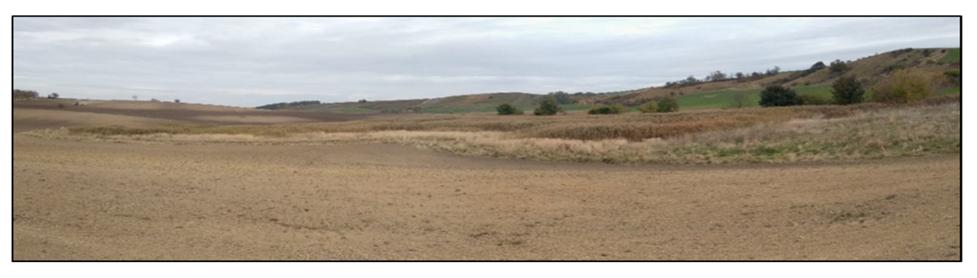
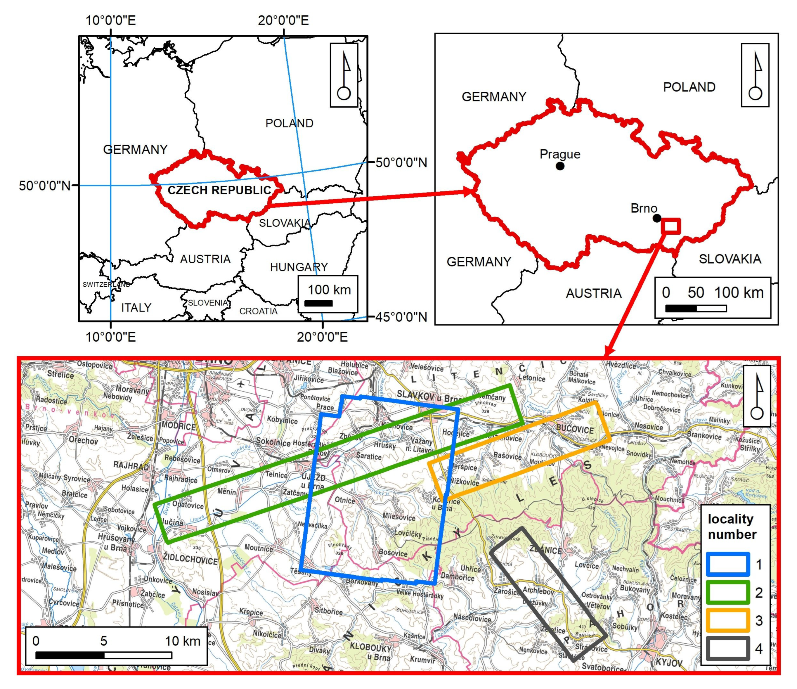
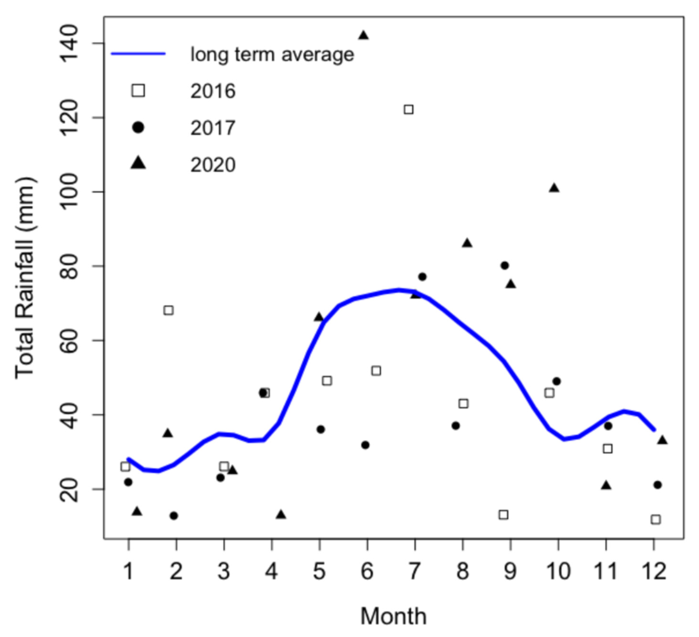
2.1. Study Area

The area of interest is located in South Moravia, SE of Brno, the extent of which corresponds to aerial hyperspectral images taken in 2016, 2017, and 2020 by the Flying Laboratory of Imaging Systems (FLIS) operated by the Global Change Research Institute.
From the geomorphological perspective, the area comprises mainly plains and hills. Elevation ranges approximately between 200 and 400 m above sea level. In the western part, the land rises from SW to NE, in the eastern part, it rises and then falls again in the NW–SE axis. The area is within a very warm-to-warm climate zone. At lower elevations, there is a typical seasonal lack of precipitation. At lower elevations, there are soils of chernozem groups, while at higher elevations, there are leptosols, luvisols, and cambisols. Around water courses, there are also fluvisols. Hydrologically, there are several subbasins which form the source area, the upper and middle parts of local water courses that flow into the Black Sea basin.
The area of interest is comprised of heavily used agricultural lands with a high proportion of fertile land. Wheat, barley, corn, and winter rape are the main crops grown, while the use of perennial fodder is low due to a reduction in livestock production. The area also includes the wine region of South Moravia. There are smaller industrial and food businesses in the area, and residents often commute to the nearby regional city of Brno for job opportunities.
A total of four locations were considered, three within one time period and one in four time periods (Figure 3). The area under consideration is an intensively farmed area with a predominance of chernozem soils in the warmest and driest climatic region of the Czech Republic. At the time of the aerial imaging campaigns, data were available on the relative saturation of the soil and the intensity of drought, as well as monthly precipitation totals in the monitored years. These data are shown in Table 1 and Figure 4.

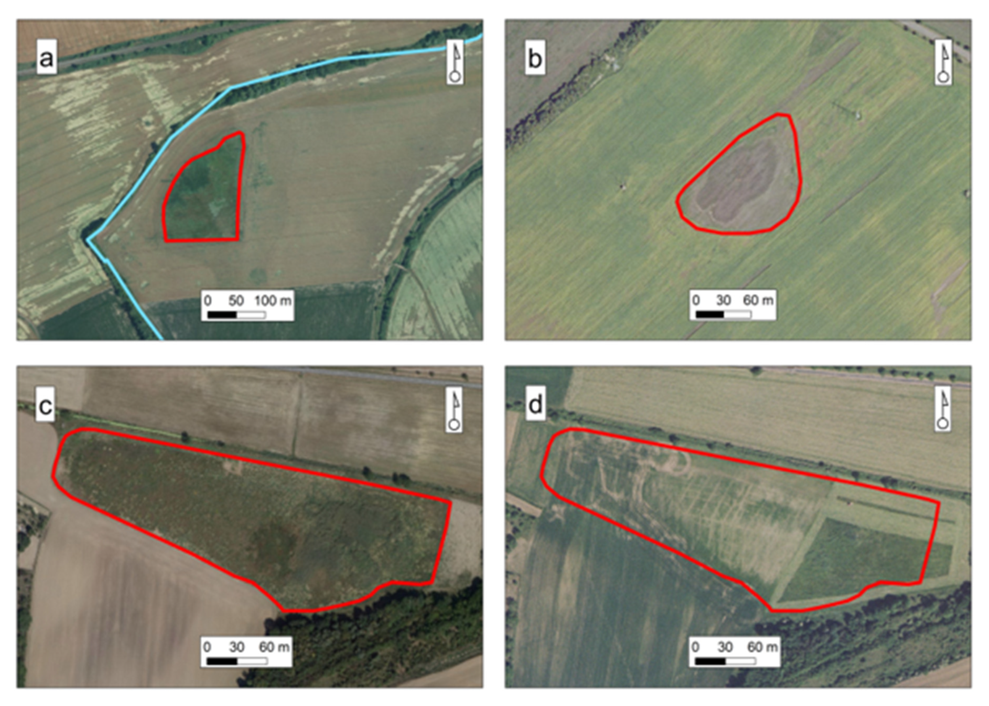
2.2. Waterlogged Areas—Specification and Data Source

The basic underlying data layer for the vectorization of waterlogged areas and subsequent analysis of spectral indices was a seamless orthophoto map of the Czech Republic from 2000 to 2020. This data layer is publicly available on the ČÚZK geoportal (Czech Land Survey and Cadastral Office) as a WMS or viewing service. A total of nine time periods were used. Specifically, these were archival orthophoto maps from 2000, 2003, 2006, 2009, 2012, 2014, 2016, 2018, and the current orthophoto from 2020. The target waterlogged areas were first visually identified within the scope of the area of interest and on individual orthophoto maps (periods) and then continuously manually vectorized in the ArcGIS software environment.
Figure 5 shows typical waterlogged areas on agricultural land at different stages of development. Figure 5a shows a waterlogged area (red polygon) on part of a soil block in the stage of developed field wetland with hygrophilous vegetation; on the surrounding soil block, there was a cereal crop. In this image, a waterlogged area is also found in the flooded area of a defunct historical pond (see the blue border). In Figure 5b, the waterlogged site is in the initial stage of field wetland development with residual stagnant water on the surface without wetland vegetation. On the surrounding area of the soil block, there is oilseed rape just before flowering. On orthophoto images, it is sometimes possible to also observe, besides the waterlogging itself, its cause, which is often non-functional subsurface drainage (Figure 5d), which shows the same location as in Figure 5c, but in a different year. In the central part, the influence of subsurface drainage in the form of a series of collection and drainage channels is evident in vegetation growth. At the same time, when comparing the local situation, the development of the waterlogged area over the years as a result of non-functional drainage can be seen.

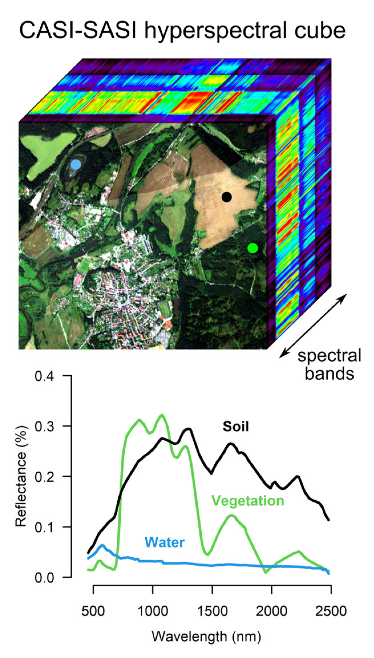
2.3. Hyperspectral Data

The spectral indices were computed from hyperspectral airborne images acquired with CASI and SASI spectroradiometers (Itres, Ltd.) on the Flying Laboratory of Imaging Systems (FLIS) operated by CzechGlobe on 30 April 2016, 27 August 2016, 19 May 2017, and 30 August 2017 (Figure 3, Locality 1), and then on 21 August 2020, in areas 2, 3, and 4 (see Figure 3).
Firstly, all images were radiometrically corrected, georeferenced, corrected for atmospheric influence, and combined into one data cube (185 spectral bands in steps of 371 and 2442 nm, with a bandwidth of 7 nm in the VNIR range and 15 nm in the SWIR range) [23]. Combination into one data cube required (Figure 6) downsampling of the spatial resolution of CASI images to match the nominal spatial resolution of SASI images (5.0 m). Apart from the actual spectral indices, the images were classified in ENVI utilizing the maximum likelihood supervised classification, differentiating between vegetation cover, bare soil, and other forms of land use.

2.4. Spectral Indices
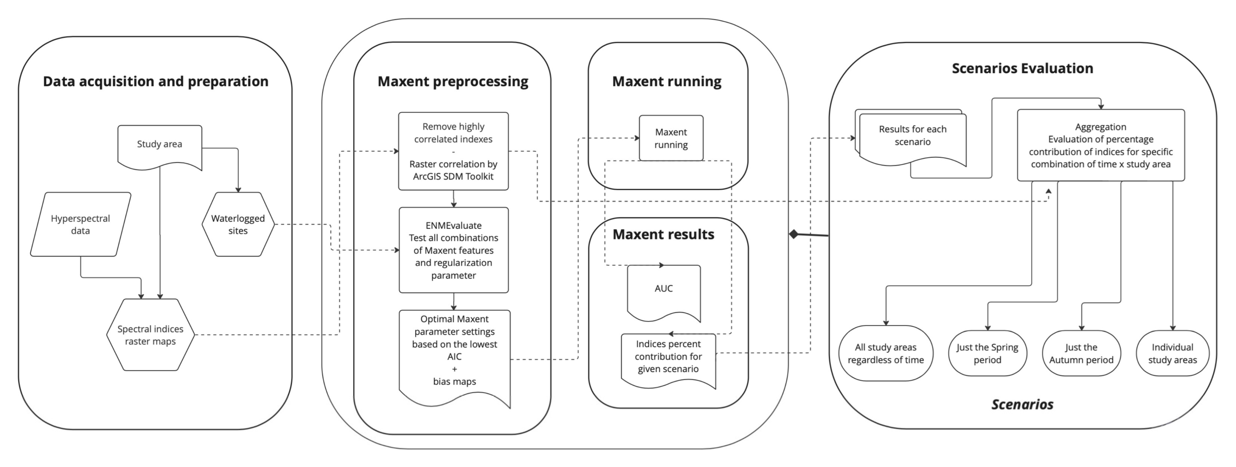
Based on professional literature [13,24,25], 33 indices were selected that cover the broadest possible range of vegetation and soil manifestations of waterlogged areas (Table 2).

2.5. Modelling

The maximum entropy model (MAXENT), which works on the basis of presence data, was used to compare the suitability of the indices. The presences, in this case, were the centroids of digitized waterlogged areas within all the areas of interest. The environmental conditions were individual hyperspectral indices.
The MAXENT model is often used in a standard parameter setting, which rarely yields the best results [50,51,52], especially in cases where the number of observations is low. Therefore, following the methodology of Warren and Seifert [53] and recommendations [54], firstly, we removed highly correlated variables (r > 0.7) and obtained reduced sets of 9–12 uncorrelated input variables from the original set of 36 variables. Using the Enmevaluate tool, we evaluated all combinations of possible dependencies (linear, quadratic, combined, threshold, stepwise) and selected the one with the lowest AIC (delta AIC = 0). Since the number of waterlogged areas in the areas of interest was small (<50), we used the leave-one-out method for cross-validation. We set the number of replications to the number of waterlogged regions in individual cases. We worked with the original resolution of hyperspectral images 5 m × 5 m when all preparatory work was completed in the ArcGIS 10.8 environment (ESRI 2019. ArcGIS Desktop: Release 10.8. Redlands, CA, USA: Environmental Systems Research Institute).
The entire procedure consists of several steps which, including the processing of results, are shown in Figure 7:
  • Finding correlation of input layers and removing highly correlated variables for all territories and each period separately; for our purposes, a value of 0.7 was chosen. Correlation was performed via the freely downloadable ArcGIS SDMToolkit extension.
  • A set of detection points (centroids of waterlogged areas) and representative uncorrelated rasters from the previous step were prepared for each territory and each period.
  • Using the Enmevaluate tool [53] in the R statistical program environment, variants of the input settings of the MAXENT program were tested precisely according to the procedure described on the website of the Integrative Evolutionary and Conservation Biology Lab (https://sites.google.com/site/thebantalab/). The best input parameters were those with the lowest Akaike information criterion (AIC) value. The result was a correlation parameter (linear, quadratic, combined, threshold, step, or combined) and a regularization parameter.
  • The MAXENT application was set according to the results of the previous step and launched.

The Method of Processing Results from the MAXENT Application

The output from the MAXENT program also includes a table evaluating the contributions of individual variables (hyperspectral indices) to the overall probability of occurrence of a waterlogged area. A total of seven cases were processed—four for site 1, each in a different time period, and one for sites 2–4 each, all in the same period.
Let us denote the evaluation of the contributions of individual indices i in a particular case j (combination of time and location) as Hij. Furthermore, Cij as a set of indices highly correlated with the index even in the case of j.
For all the k indices that were not selected for modelling in the MAXENT program for the individual case j, we set Hkj as follows:
Hkj = Hijcor(k,i),
where cor represents the correlation of the sought variable k with the selected representative i in the case of j.
The resulting evaluation of the indices was subsequently carried out in several variants:
  • All cases, regardless of period and location;
  • Spring period, regardless of location;
  • Autumn period, regardless of location;
  • Site 1 alone, regardless of the period;
  • Site 1 alone in spring and autumn;
  • The year 2020 alone.
For each variant, an average contribution to the probability of identifying a waterlogged area was obtained.

3. Results

The MAXENT model provides several types of results. The general accuracy of the prediction of waterlogged areas is determined by the value of the area under curve (AUC) or the curve of operating characteristics (ROC). The best in this respect was case 1 in the spring of 2016, followed, in general, by 2017 (Table 3).
MAXENT also enables the comparison of the significance of variables based on indicators, e.g., a jackknife test of the training set or the test set concerning the gain function (accuracy improvement) or the overall AUC value. We used the expression of the so-called contribution of variability, which shows to what extent individual variables contribute to the general determination of the probability of the observed phenomenon, in this case, the waterlogged area. Table 4 shows these contributions in particular periods and locations; Table 5 then provides the derived aggregated results for the individually processed variants, which are the average of the variable contributions for several cases.
In general, indices relating to chlorophyll content, MCARI (31.8%), CARI (23.6%), and TCARI2 (24.3%), proved to be the best for identifying waterlogged areas. In springtime, the NVI index is the most successful, followed, again, by the indices already mentioned.
Another output of MAXENT is so-called reaction curves, where we can see the effect of a specific value of the monitored variable on the occurrence probability. The reaction curve of the generally best index (according to the analysis)—NVI—shows a significant decrease in probability with values further away from zero. Therefore, waterlogged surfaces are best determined by values with an index close to 0 (see Figure 8). Another example can be the most successful MCARI index from the autumn of 2017, when its contribution to variability was up to 93% (see Figure 9). The threshold here is represented by values greater than 600.
All the MAXENT results can be found in the Figshare Digital Repository (https://doi.org/10.6084/m9.figshare.21710309.v1, accessed on 12 December 2022).

4. Discussion

During the post-war collectivization of the agricultural sector, significant changes occurred in the Czech landscape. The size of blocks of arable land increased, and the average block size is currently greater than 10 ha [55]. This period also saw the homogenization of the landscape caused by the elimination of fragments of woody stands and other nonproductive areas [56,57]. These conditions led to intensified erosion processes and runoff events leading to reservoir silting [58].
The result of landscape homogenization is large blocks of agricultural land, on which waterlogged areas are often present with a minimal or limited production function (Figure 2). At the same time, however, they can be precious from a nonproduction point of view. They retain water in the landscape, contribute to slowing down the runoff, and are centres of increased biodiversity and genetic integrity [8]. They often take on the character of periodic (ephemeral) wetlands. This tends to be a problem when defining their boundaries due to their unstable (periodic/episodic) occurrence [59].
Waterlogging on these sites has various causes. In general, however, it can be said that the leading cause is local physical–geographical factors such as terrain morphology, geological and soil conditions, groundwater level, etc. [60].
The aim of our research was to determine whether it is possible to identify waterlogged areas on agricultural land by means of spectral indices, and with what sensitivity. The analysis made use of spectral indices falling into different categories characterizing the structure, foliage cover, level of chlorophyll and water in plants and in the soil, which could indicate the presence of a waterlogged area. Of course, this range could be expanded to include other spectral indices which are often more difficult to process. However, our intention was to analyse the most commonly used indices, ideally those which can be processed with a certain degree of inaccuracy even without more detailed hyperspectral data using commonly available multispectral data, e.g., from Sentinel-2. The training set was waterlogged areas as they had been identified on the basis of archival and contemporary orthophoto maps.
For our analysis, we used the MAXENT model, which is generally used more for modelling the spatial distribution of species, where it is currently among the most commonly applied models and where it also achieves the most accurate results [52]. This, however, assumes the correct setting of model parameters. For this purpose, we used the Enmevaluate tool, which allows the evaluation of a combination of MAXENT settings based on the lowest Akaike information criterion (AIC). The preselection of input variables for analysis is particularly ambiguous. MAXENT is not susceptible to collinearity; unlike other statistical methods, it is often perceived more as a machine learning tool, and no preselection is necessary [51]. Nevertheless, especially in ecological applications, there is a reduction in input variables, usually through PCA analysis or variable correlation [51], which was also used in our article.
MAXENT allows the creation of models with linear, quadratic, combined, threshold, and step effect of variables on the probability of identification of the observed phenomenon (waterlogged area). The Enmevaluate tool was used as the best setting for input data based on delta AIC depending on the site and period of interest. The type of dependence determines this setting—in our case, it was threshold, quadratic, and linear dependence—and also by choosing the regularization parameter, which is a kind of penalty for overfitting the data. Threshold dependence means a specific threshold value at which linear dependence becomes evident.
Waterlogged areas/water content are/is best detected by three indices considering chlorophyll (MCARI, CARI, and TCARI2). The other indices (DVI, EVI, MTVI2, NDMI, OSAVI, PRI, RDVO, WI_NDVI) were identified as not being very sensitive for the detection of waterlogged areas, i.e., with the lowest average percentage contribution. These less sensitive indices are based on parameters such as plant physiognomy and LAI (for the EVI index).
A high spectral resolution measure, defined as the chlorophyll absorption ratio index (CARI), was developed to minimize the effects of non-photosynthetic materials in the remote estimates of photosynthetically active radiation [61]. Daughtry et al. [29] simplified the CARI index to minimize the combined effects of soil and non-photosynthetic surfaces, leading to the MCARI index.
The modified chlorophyll absorption in reflectance index (MCARI) measures the depth of chlorophyll absorption. It is susceptible to variations in chlorophyll concentration and leaf area index (LAI). MCARI values are not affected by illumination conditions, and the background reflectance from soil and other non-photosynthetic materials was observed. However, Daughtry et al. [29] also showed that the MCARI is influenced by background reflectance and parameters such as LAI and LAI–chlorophyll interaction. Haboudan et al. [30] also showed that the MCARI is sensitive to non-photosynthetic materials, especially at low chlorophyll concentration. That is why the TCARI2 index was created, which compensates for soil reflection and non-photosynthetic components and increases sensitivity at low chlorophyll values.
For the spring period (May), our analysis evaluated the NVI index (new vegetation index) as the most advantageous index. This was initially developed to better distinguish wheat from other crops based on the difference between peak radiances at 777 and 747 nm with reflected radiance at 673 nm in the red area [41]. This index is also described by Liang et al. [62] when studying the leaf area index (LAI) as an indicator of vegetation growth.
The narrow link between relative water content in plants and soil water content had already been revealed by Fischer [63], who suggested plants as an indirect indicator of water content in the soil. Moisture stress inhibits leaf water and chlorophyll content [64,65]. Water stress damages the cell membrane and affects the stability of chlorophyll [66]. Hence, chlorophyll as a parameter may also be used to assess crop water status.
A decreased Chl a/b ratio was also observed under water stress in a study by Zhang et al. [67]. These results indicate that drought can result in damage to the photosynthetic apparatus and may affect other physiological parameters (gas exchange, Chl a/b ratio, water use efficiency, light compensation and light saturation points, maximum photosynthetic rates and dark respiration rates.
The foliar element of the vegetation canopy structure (LAI) aggregates leaf level characteristics and is closely connected with canopy density, physiological processes, and structural traits of leaves for photosynthesis [68]. The value is sensitive to several environmental factors, including moisture [69]. The value increases with moisture, but the relationship to temperature is not straightforward. Global remote sensing also revealed correlations with elevation and precipitation [70,71]. Leaf physiological dynamics are essential indicators of vegetation condition and ecosystem function both from a local and landscape points of view [72,73].
We consider this as the main reason for the indices based on chlorophyll and LAI showing high sensitivity in identifying waterlogged areas. Yet, there are differences between the chlorophyll and LAI-based indices in terms of the detection ability at different times of the year. There is a striking difference between the detection abilities of LAI-based indices in springtime. Chlorophyll-based indices are generally more successful, but achieve the best results in autumn. Both chlorophyll and LAI are important indicators of vegetation conditions and, hence, environmental factors in remote sensing [74,75,76]. However, experimental evaluation of the differences in informative value is beyond the scope of our study, and it is recommended that this be addressed in separate further research.
As part of our analysis, both spectral indices understood as broad-band and narrow-band were used. However, all the indices were derived from hyperspectral data based on the exact wavelengths listed in Table 2. The disadvantage of hyperspectral data is the high purchase price and only partial spatial and temporal coverage of the studied areas.
Some hyperspectral indices can also be derived, to a certain extent, based on multispectral data, e.g., the SENTINEL-2 satellite. Of course, this is only possible if the reflectance in specific wavelengths used for hyperspectral indices can be derived from multispectral data within the considered wavelength bandwidth of the hyperspectral index. In our case, one of the four most advantageous indices—MCARI, CARI, TCARI2, and NVI—can be used with a certain degree of inaccuracy, e.g., the CARI index using wavelengths 700 and 670 nm, which most closely corresponds to band 5—vegetation red edge of the Sentinel-2A satellite (medium wavelength, 704.1 nm, bandwidth, 15 nm), or band 4—red (central wavelength, 664.6 nm, bandwidth, 31 nm). The same is true for the MCARI and tcari2 indices, where, in addition to the wavelengths mentioned for the CARI, a wavelength of 550 nm is also used, which corresponds to band 3—green (central wavelength, 559.8 nm, bandwidth, 36 nm). The NVI index uses wavelengths of 777, 747, and 673 nm, instead of which we can use Sentinel-2A satellite’s band 7—vegetation red edge (central wavelength, 782.8 nm, bandwidth 20 nm), band 6—vegetation red edge (central wavelength, 740.5 nm, bandwidth, 15 nm), and band 4—red (central wavelength, 664.6 nm, bandwidth, 31 nm). With the NVI index, however, this inaccuracy is already quite significant; it is recommended for use only in steps of up to 10 nm [41]; the results, in this case, would be highly debatable.
Despite this, we consider this direction of research to be very promising. In subsequent research, we will focus more closely on the difference between hyperspectral and spectral images.
Of course, the results can also be influenced by precipitation, soil moisture at the time of aerial imaging, and the degree of widespread drought, which can vary considerably in individual years and seasons. Therefore, in addition to spatial diversification, we also processed different periods, covering an above-average rainfall year (2020) and below-average rainfall years (2016 and 2017), as documented (Figure 4). The relative saturation of the soil a few days before the aerial campaign in the spring of 2016 and 2017 was above average, i.e., with sufficient soil moisture, which corresponds to the higher total precipitation of the given month. The autumn periods of 2017 and 2018 were different. While relative soil saturation remained above average in 2016, in 2017, it was the lowest of all the monitored periods and reached around 30%. In terms of precipitation, both years were similar. However, the stormy July of 2016 was reflected in saturation intensity, so the soil did not show any signs of danger from drought. In terms of the accuracy of the MAXENT model forecast, the spring periods were generally more successful (AUC = 0.792 and 0.715, respectively) when soil saturation was generally higher; however, similar success (AUC = 0.733) was also achieved in the autumn of 2017, when the soil suffered from a lack of moisture. Differentiation of the success of individual spectral indices may also relate to this. In the wet spring period, the NVI index sensitive to foliage cover was the most sensitive in terms of waterlogged areas.
On the other hand, indices related to the amount of chlorophyll, distinguishability of bare soil, and soil moisture (OSAVI) performed best in the dry autumn period. The year 2020 was above average in terms of precipitation, which was also evident in the autumn period when the soil did not suffer from a lack of moisture. However, this is precisely why the model results are inconclusive in this period. More extensive aerial campaigns would be needed to confirm the relationship between season, relative soil saturation, and predictive accuracy of models.

5. Conclusions

The overall results can be summarized as follows:
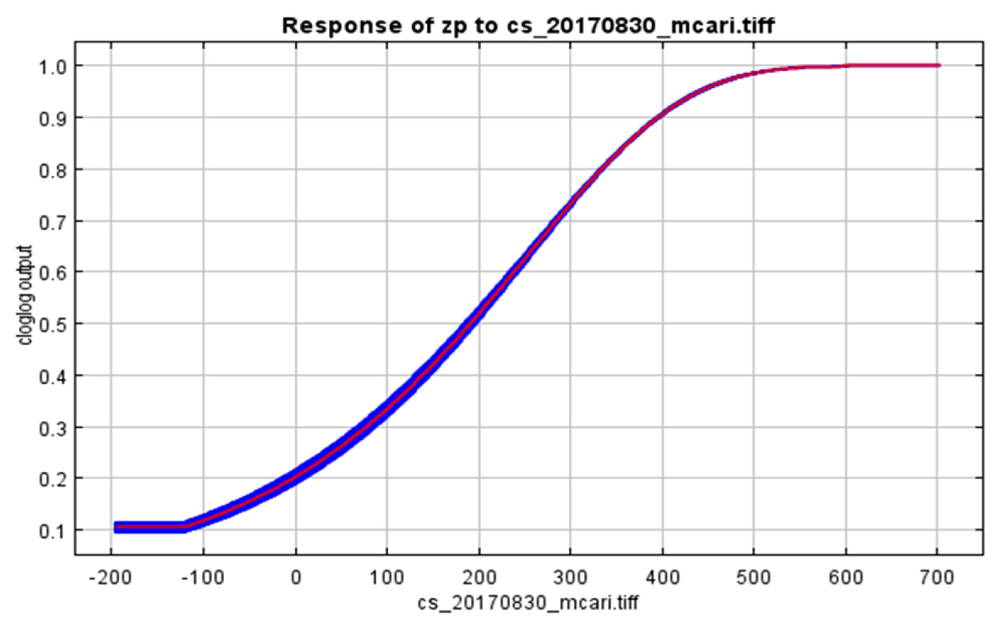
  • For the identification of wetland areas, only some of the commonly used hyperspectral indices can be used. In this regard, chlorophyll-based indices worked best for us, with a higher amount of chlorophyll representing a higher probability of a wetland area.
  • Although chlorophyll-based indices can be used regardless of the season, better results were achieved in springtime with the NVI index, which represents indices focusing on LAI. A higher probability of occurrence corresponded to low LAI values, indicating low leaf coverage.
  • The overall sensitivity of the best indices is statistically significant but does not reach high values. This shows that the use of remote sensing is suitable for the primary selection of wetland areas, which must still be verified in the field.
  • The research shows that the exact determination of waterlogged areas in the agricultural landscape is not easy, especially when there is a lack of available hyperspectral data. Such data are not yet readily available in the Czech Republic or other countries. Only recently have the DESIS spectroradiometer on the ISS [77] and two hyperspectral satellites, the Italian PRISMA [78] and the German EnMAP [79], started to supply hyperspectral data. Together with the proposed Copernicus satellite mission CHIME with global coverage [80], we expect hyperspectral data to become more important for various land surface applications. An alternative could be the use of multispectral data using available satellites. However, practical use of such data, due to the lower sensitivity of spectral indices, will be the subject of further research.
  • A valuable result, although difficult to interpret biologically, is the role of LAI expressed by the NVI index and the role of chlorophyll in identifying wetland areas. Interpretation cannot be achieved at the level of remote sensing, and further research based on field experiments will be necessary for clarification.
The use of remote sensing can be valuable for both policymakers and practitioners as it can be used to make an initial selection of areas where adaptation and retention measures can be planned and implemented. This remote sensing must be followed by more detailed reconnaissance of the terrain where local knowledge of natural and socio-economic conditions can help in the selection and implementation of the most appropriate measures. These can include the construction of small reservoirs or semiarid polders, as well as the design of nature-based measures, such as the revitalization of rivers, wetlands, or periodic ponds, the aim of which is to improve the state of the landscape affected by climate change and more frequent hydrometeorological extremes.

Author Contributions

Conceptualization, M.B., B.Š., P.N. and M.Z.; methodology, M.B.; software, M.B. and T.H.; validation, M.B., M.Z., P.N., L.H. and B.Š.; formal analysis, M.B.; investigation, M.B., B.Š., P.N. and M.Z.; resources, L.H. and T.H.; data curation, M.B. and T.H.; writing—original draft preparation, M.B., B.Š., P.N., M.Z. and L.H; writing—review and editing, M.B., B.Š. P.N., M.Z. and L.H.; visualization, M.B. and P.N.; supervision, B.Š.; project administration, M.B. and B.Š.; funding acquisition, B.Š. All authors have read and agreed to the published version of the manuscript.

Funding

This research was funded by the Ministry of Agriculture of the Czech Republic supporting the research through grants from the National Agency for Agricultural Research (QK21010328, “Potential for the Development of Small Water Bodies in the Landscape as Adaptation Measures to Eliminate Hydrometeorological Extremes”, and by the Technology Agency of the Czech Republic (SS02030018, Centre for Landscape and Biodiversity).

Institutional Review Board Statement

Not applicable.

Data Availability Statement

Not applicable.

Conflicts of Interest

The authors declare no conflict of interest.

References

  1. Trnka, M.; Brázdil, R.; Vizina, A.; Dobrovolný, P.; Mikšovský, J.; Štěpánek, P.; Hlavinka, P.; Řezníčková, L.; Žalud, Z. Droughts and Drought Management in the Czech Republic in a Changing Climate. In Drought and Water Crises, 2nd ed.; Wilhite, D.A., Pulwarty, R.S., Eds.; Integrating Science, Management, and Policy; CRC Press: Boca Raton, FL, USA; Taylor & Francis: UK, 2017; pp. 461–480. ISBN 978-1-138-03564-5. [Google Scholar] [CrossRef]
  2. Brázdil, R.; Rezníčková, L.; Valášek, H.; Havlíček, M.; Dobrovolný, P.; Soukalová, E.; Rehánek, T.; Skokanová, H. Fluctuations of Floods of the River Morava (Czech Republic) in the 1691–2009 Period: Interactions of Natural and Anthropogenic Factors. Hydrol. Sci. J. 2011, 56, 468–485. [Google Scholar] [CrossRef]
  3. Trnka, M.; Brázdil, R.; Možný, M.; Štěpánek, P.; Dobrovolný, P.; Zahradníček, P.; Balek, J.; Semerádová, D.; Dubrovský, M.; Hlavinka, P.; et al. Soil Moisture Trends in the Czech Republic between 1961 and 2012. Int. J. Climatol. 2015, 35, 3733–3747. [Google Scholar] [CrossRef]
  4. Brázdil, R.; Zahradníček, P.; Dobrovolný, P.; Štěpánek, P.; Trnka, M. Observed Changes in Precipitation during Recent Warming: The Czech Republic, 1961–2019. Int. J. Climatol. 2021, 41, 3881–3902. [Google Scholar] [CrossRef]
  5. Pavelková, R.; Frajer, J.; Havlíček, M.; Netopil, P.; Rozkošný, M.; David, V.; Dzuráková, M.; Šarapatka, B. Historical Ponds of the Czech Republic: An Example of the Interpretation of Historic Maps. J. Maps 2016, 12, 551–559. [Google Scholar] [CrossRef] [Green Version]
  6. Kulhavý, Z.; Doležal, F.; Fučík, P.; Kulhavý, F.; Kvítek, T.; Muzikář, R.; Soukup, M.; Švihla, V. Management of Agricultural Drainage Systems in the Czech Republic. Irrig. Drain. 2007, 56, S141–S149. [Google Scholar] [CrossRef]
  7. Kulhavý, Z.; Žaloudík, J.; Tlapáková, L.; Burešová, Z.; Eichler, J.; Čmelík, M. Identification of Subsurface Drainage Systems by Air Photographs. In Proceedings of the ICID 21st European Regional Conference, Frankfurt, Germany; Slubice, Poland, 15–19 May 2005. [Google Scholar]
  8. Němec, R.; Dřevojan, P.; Šumberová, K. Wetlands on Arable Land in Znojmo Region as a Refuge of Important and Rare Vascular Plants. Thayensia 2014, 11, 3–76. [Google Scholar]
  9. Churko, G.; Gramlich, A.; Walter, T. Vascular Plant and Ground Beetle Diversity on Wet Arable Land versus Conventional Crop Fields. Basic Appl. Ecol. 2021, 53, 86–99. [Google Scholar] [CrossRef]
  10. Sychra, J.; Čamlík, G.; Merta, L.; Zavadil, V.; Devánová, A. Temporal Field Wetlands as Biodiversity Hot Spots in Agricultural Landscape in the Czech Republic. In Proceedings of the 10 Symposium for European Freshwater Sciences, Olomouc, Czech Republic, 2–7 July 2017. [Google Scholar]
  11. Wu, Q. GIS and Remote Sensing Applications in Wetland Mapping and Monitoring. Compr. Geogr. Inf. Syst. 2018, 3, 140–157. [Google Scholar] [CrossRef]
  12. Dorigo, W.A.; Zurita-Milla, R.; de Wit, A.J.W.; Brazile, J.; Singh, R.; Schaepman, M.E. A Review on Reflective Remote Sensing and Data Assimilation Techniques for Enhanced Agroecosystem Modeling. Int. J. Appl. Earth Obs. Geoinf. 2007, 9, 165–193. [Google Scholar] [CrossRef]
  13. Giovos, R.; Tassopoulos, D.; Kalivas, D.; Lougkos, N.; Priovolou, A. Remote Sensing Vegetation Indices in Viticulture: A Critical Review. Agriculture 2021, 11, 457. [Google Scholar] [CrossRef]
  14. Zhao, D.; Huang, L.; Li, J.; Qi, J. A Comparative Analysis of Broadband and Narrowband Derived Vegetation Indices in Predicting LAI and CCD of a Cotton Canopy. ISPRS J. Photogramm. Remote Sens. 2007, 62, 25–33. [Google Scholar] [CrossRef]
  15. Gamon, J.A.; Somers, B.; Malenovský, Z.; Middleton, E.M.; Rascher, U.; Schaepman, M.E. Assessing Vegetation Function with Imaging Spectroscopy. Surv. Geophys. 2019, 40, 489–513. [Google Scholar] [CrossRef] [Green Version]
  16. Mutanga, O.; Skidmore, A.K. Narrow Band Vegetation Indices Overcome the Saturation Problem in Biomass Estimation. Int. J. Remote Sens. 2010, 25, 3999–4014. [Google Scholar] [CrossRef]
  17. Ray, D.; Behera, M.D.; Jacob, J. Evaluating Ecological Niche Models: A Comparison Between Maxent and GARP for Predicting Distribution of Hevea Brasiliensis in India. Proc. Natl. Acad. Sci. India Sect. B Biol. Sci. 2018, 88, 1337–1343. [Google Scholar] [CrossRef]
  18. Belgiu, M.; Drăgu, L. Random Forest in Remote Sensing: A Review of Applications and Future Directions. ISPRS J. Photogramm. Remote Sens. 2016, 114, 24–31. [Google Scholar] [CrossRef]
  19. Huang, G.B.; Zhu, Q.Y.; Siew, C.K. Extreme Learning Machine: A New Learning Scheme of Feedforward Neural Networks. In Proceedings of the IEEE International Conference on Neural Networks, Budapest, Hungary, 25–29 July 2004; Volume 2. [Google Scholar]
  20. Fitzpatrick, M.C.; Gove, A.D.; Sanders, N.J.; Dunn, R.R. Climate Change, Plant Migration, and Range Collapse in a Global Biodiversity Hotspot: The Banksia (Proteaceae) of Western Australia. Glob. Chang. Biol. 2008, 14, 1337–1352. [Google Scholar] [CrossRef]
  21. Beaumont, L.J.; Hughes, L. Potential Changes in the Distributions of Latitudinally Restricted Australian Butterfly Species in Response to Climate Change. Glob. Chang. Biol. 2002, 8, 954–971. [Google Scholar] [CrossRef]
  22. Phillips, S.J.; Dudík, M.; Schapire, R.E. A Maximum Entropy Approach to Species Distribution Modeling. In Proceedings of the 21st International Conference on Machine Learning—ICML ’04, Banff, AB, Canada, 4–8 July 2004; Volume 83. [Google Scholar] [CrossRef] [Green Version]
  23. Hanuš, J.; Fabiánek, T.; Fajmon, L. Potential of Airborne Imaging Spectroscopy at Czechglobe. Int. Arch. Photogramm. Remote Sens. Spat. Inf. Sci. 2016, XLI-B1, 15–17. [Google Scholar] [CrossRef] [Green Version]
  24. Ge, X.; Wang, J.; Ding, J.; Cao, X.; Zhang, Z.; Liu, J.; Li, X. Combining UAV-Based Hyperspectral Imagery and Machine Learning Algorithms for Soil Moisture Content Monitoring. PeerJ 2019, 7, e6926. [Google Scholar] [CrossRef]
  25. Main, R.; Cho, M.A.; Mathieu, R.; O’Kennedy, M.M.; Ramoelo, A.; Koch, S. An Investigation into Robust Spectral Indices for Leaf Chlorophyll Estimation. ISPRS J. Photogramm. Remote Sens. 2011, 66, 751–761. [Google Scholar] [CrossRef]
  26. Tian, Y.; Yao, X.; Yang, J.; Cao, W.; Zhu, Y. Extracting Red Edge Position Parameters from Ground- and Space-Based Hyperspectral Data for Estimation of Canopy Leaf Nitrogen Concentration in Rice. Plant Prod. Sci. 2015, 14, 270–281. [Google Scholar] [CrossRef]
  27. Huete, A.R.; Liu, H.Q.; Batchily, K.; van Leeuwen, W. A Comparison of Vegetation Indices over a Global Set of TM Images for EOS-MODIS. Remote Sens. Environ. 1997, 59, 440–451. [Google Scholar] [CrossRef]
  28. Yao, X.; Wang, N.; Liu, Y.; Cheng, T.; Tian, Y.; Chen, Q.; Zhu, Y. Estimation of Wheat LAI at Middle to High Levels Using Unmanned Aerial Vehicle Narrowband Multispectral Imagery. Remote Sens. 2017, 9, 1304. [Google Scholar] [CrossRef] [Green Version]
  29. Daughtry, C.S.T.; Walthall, C.L.; Kim, M.S.; de Colstoun, E.B.; McMurtrey, J.E. Estimating Corn Leaf Chlorophyll Concentration from Leaf and Canopy Reflectance. Remote Sens. Environ. 2000, 74, 229–239. [Google Scholar] [CrossRef]
  30. Haboudane, D.; Miller, J.R.; Tremblay, N.; Zarco-Tejada, P.J.; Dextraze, L. Integrated Narrow-Band Vegetation Indices for Prediction of Crop Chlorophyll Content for Application to Precision Agriculture. Remote Sens. Environ. 2002, 81, 416–426. [Google Scholar] [CrossRef]
  31. Sims, D.A.; Gamon, J.A. Relationships between Leaf Pigment Content and Spectral Reflectance across a Wide Range of Species, Leaf Structures and Developmental Stages. Remote Sens. Environ. 2002, 81, 337–354. [Google Scholar] [CrossRef]
  32. Qi, J.; Chehbouni, A.; Huete, A.R.; Kerr, Y.H.; Sorooshian, S. A Modified Soil Adjusted Vegetation Index. Remote Sens. Environ. 1994, 48, 119–126. [Google Scholar] [CrossRef]
  33. Liang, L.; Di, L.; Zhang, L.; Deng, M.; Qin, Z.; Zhao, S.; Lin, H. Estimation of Crop LAI Using Hyperspectral Vegetation Indices and a Hybrid Inversion Method. Remote Sens. Environ. 2015, 165, 123–134. [Google Scholar] [CrossRef]
  34. Martínez, M.; Martínez, M.E.; Martínez, E.; Renza, D. Detection of Changes in Natural Aquifer Reservoirs Based on the Index of Drought. IEEE Lat. Am. Trans. 2017, 15, 2059–2063. [Google Scholar] [CrossRef]
  35. Hunt, E.R., Jr.; Wang, L.; Qu, J.J.; Hao, X. Remote Sensing of Fuel Moisture Content from Canopy Water Indices and Normalized Dry Matter Index. J. Appl. Remote. Sens. 2012, 6, 061705. [Google Scholar] [CrossRef]
  36. Barnes, E.; Colaizzi, P.; Haberland, J.; Waller, P. Coincident Detection of Crop Water Stress, Nitrogen Status, and Canopy Density Using Ground Based Multispectral Data. In Proceedings of the Fifth International Conference on Precision Agriculture, Bloomington, MN, USA, 16–19 July 2000. [Google Scholar]
  37. Tucker, C.J. Red and Photographic Infrared Linear Combinations for Monitoring Vegetation. Remote Sens. Environ. 1979, 8, 127–150. [Google Scholar] [CrossRef] [Green Version]
  38. Gitelson, A.; Merzlyak, M.N. Quantitative Estimation of Chlorophyll-a Using Reflectance Spectra: Experiments with Autumn Chestnut and Maple Leaves. J. Photochem. Photobiol. B 1994, 22, 247–252. [Google Scholar] [CrossRef]
  39. Qiao, C.; Luo, J.; Sheng, Y.; Shen, Z.; Zhu, Z.; Ming, D. An Adaptive Water Extraction Method from Remote Sensing Image Based on NDWI. J. Indian Soc. Remote Sens. 2012, 40, 421–433. [Google Scholar] [CrossRef]
  40. Wang, L.; Qu, J.J. NMDI: A Normalized Multi-Band Drought Index for Monitoring Soil and Vegetation Moisture with Satellite Remote Sensing. Geophys. Res. Lett. 2007, 34, 1–5. [Google Scholar] [CrossRef]
  41. Gupta, R.K.; Vijayan, D.; Prasad, T.S. New Hyperspectral Vegetation Characterization Parameters. Adv. Space Res. 2001, 28, 201–206. [Google Scholar] [CrossRef]
  42. Rondeaux, G.; Steven, M.; Baret, F. Optimization of Soil-Adjusted Vegetation Indices. Remote Sens. Environ. 1996, 55, 95–107. [Google Scholar] [CrossRef]
  43. Peñuelas, J.; Gamon, J.A.; Griffin, K.L.; Field, C.B. Assessing Community Type, Plant Biomass, Pigment Composition, and Photosynthetic Efficiency of Aquatic Vegetation from Spectral Reflectance. Remote Sens. Environ. 1993, 46, 110–118. [Google Scholar] [CrossRef]
  44. Roujean, J.L.; Breon, F.M. Estimating PAR Absorbed by Vegetation from Bidirectional Reflectance Measurements. Remote Sens. Environ. 1995, 51, 375–384. [Google Scholar] [CrossRef]
  45. Guyot, G.; Baret, F. Utilisation de La Haute Resolution Spectrale Pour Suivre l’etat Des Couverts Vegetaux. J. Chem. Inf. Model 1988, 53, 279–286. [Google Scholar]
  46. Wu, C.; Niu, Z.; Tang, Q.; Huang, W. Estimating Chlorophyll Content from Hyperspectral Vegetation Indices: Modeling and Validation. Agric. For. Meteorol. 2008, 148, 1230–1241. [Google Scholar] [CrossRef]
  47. Broge, N.H.; Leblanc, E. Comparing Prediction Power and Stability of Broadband and Hyperspectral Vegetation Indices for Estimation of Green Leaf Area Index and Canopy Chlorophyll Density. Remote Sens. Environ. 2001, 76, 156–172. [Google Scholar] [CrossRef]
  48. Vogelmann, J.E.; Rock, B.N.; Moss, D.M. Red Edge Spectral Measurements from Sugar Maple Leaves. Int. J. Remote Sens. 2007, 14, 1563–1575. [Google Scholar] [CrossRef]
  49. McCall, D.S.; Zhang, X.; Sullivan, D.G.; Askew, S.D.; Ervin, E.H. Enhanced Soil Moisture Assessment Using Narrowband Reflectance Vegetation Indices in Creeping Bentgrass. Crop. Sci. 2017, 57, S161–S168. [Google Scholar] [CrossRef]
  50. Elith, J.; Phillips, S.J.; Hastie, T.; Dudík, M.; Chee, Y.E.; Yates, C.J. A Statistical Explanation of MaxEnt for Ecologists. Divers Distrib. 2011, 17, 43–57. [Google Scholar] [CrossRef]
  51. Merow, C.; Smith, M.J.; Silander, J.A. A Practical Guide to MaxEnt for Modeling Species’ Distributions: What It Does, and Why Inputs and Settings Matter. Ecography 2013, 36, 1058–1069. [Google Scholar] [CrossRef]
  52. Morales, N.S.; Fernández, I.C.; González, V.-B. MaxEnt’s Parameter Configuration and Small Samples: Are We Paying Attention to Recommendations? A Systematic Review. PeerJ 2017, 2017, e3093. [Google Scholar] [CrossRef]
  53. Warren, D.L.; Seifert, S.N. Ecological Niche Modeling in Maxent: The Importance of Model Complexity and the Performance of Model Selection Criteria. Ecol. Appl. 2011, 21, 335–342. [Google Scholar] [CrossRef] [Green Version]
  54. Radosavljevic, A.; Anderson, R.P. Making Better Maxent Models of Species Distributions: Complexity, Overfitting and Evaluation. J. Biogeogr. 2014, 41, 629–643. [Google Scholar] [CrossRef]
  55. Fiener, P.; Dostál, T.; Krása, J.; Schmaltz, E.; Strauss, P.; Wilken, F. Operational USLE-Based Modelling of Soil Erosion in Czech Republic, Austria, and Bavaria—Differences in Model Adaptation, Parametrization, and Data Availability. Appl. Sci. 2020, 10, 3647. [Google Scholar] [CrossRef]
  56. Šarapatka, B.; Štěrba, O. Optimization of Agriculture in Relation to the Multifunctional Role of the Landscape. Landsc. Urban Plan 1998, 41, 145–148. [Google Scholar] [CrossRef]
  57. Skokanová, H.; Netopil, P.; Havlíček, M.; Šarapatka, B. The Role of Traditional Agricultural Landscape Structures in Changes to Green Infrastructure Connectivity. Agric. Ecosyst. Environ. 2020, 302, 107071. [Google Scholar] [CrossRef]
  58. Krasa, J.; Dostal, T.; van Rompaey, A.; Vaska, J.; Vrana, K. Reservoirs’ Siltation Measurments and Sediment Transport Assessment in the Czech Republic, the Vrchlice Catchment Study. Catena 2005, 64, 348–362. [Google Scholar] [CrossRef]
  59. Richter, P. Mokřady Na Archivních Mapových Podkladech. Vodohospodářské Tech. Ekon. Inf. 2020, 62, 30–37. [Google Scholar] [CrossRef]
  60. Pavelková Chmelová, R.; Frajer, J.; Netopil, P.; David, V.; Dzuráková, M.; Havlíček, M.; Hůla, P.; Peterková, L.; Rozkošný, M.; Šarapatka, B.; et al. Historické Rybníky České Republiky: Srovnání Současnosti Se Stavem v 2. Polovině 19. Století., 1st ed.; Výzkumný ústav vodohospodářský, T.G. Masaryka: Praga, Czech Republic, 2014; Volume 1. [Google Scholar]
  61. Kim, M.S. The Use of Narrow Spectral Bands for Improving Remote Sensing Estimations of Fractionally Absorbed Photosynthetically Active Radiation (Fapar). Master’s Thesis, University of Maryland, College Park, MD, USA, 1994. [Google Scholar]
  62. Liang, L.; Huang, T.; Di, L.; Geng, D.; Yan, J.; Wang, S.; Wang, L.; Li, L.; Chen, B.; Kang, J. Influence of Different Bandwidths on LAI Estimation Using Vegetation Indices. IEEE J. Sel. Top. Appl. Earth Obs. Remote Sens. 2020, 13, 1494–1502. [Google Scholar] [CrossRef]
  63. Fischer, R.A. The Effect of Water Stress at Various Stages of Development on Yield Processes in Wheat. Plant Response Clim. Factors 1973, 1973, 233–241. [Google Scholar]
  64. Sarker, A.M.; Rahman, M.S.; Paul, N.K. Effect of Soil Moisture on Relative Leaf Water Content, Chlorophyll, Proline and Sugar Accumulation in Wheat. J. Agron. Crop. Sci. 1999, 183, 225–229. [Google Scholar] [CrossRef]
  65. Sampathkumar, T.; Pandian, B.J.; Jeyakumar, P.; Manickasundaram, P. Effect of Deficit Irrigation on Yield, Relative Leaf Water Content, Leaf Proline Accumulation and Chlorophyll Stability Index of Cotton-Maize Cropping Sequence. Exp. Agric. 2014, 50, 407–425. [Google Scholar] [CrossRef]
  66. Blackman, S.A.; Obendorf, R.L.; Leopold, A.C. Desiccation Tolerance in Developing Soybean Seeds: The Role of Stress Proteins. Physiol. Plant 1995, 93, 630–638. [Google Scholar] [CrossRef]
  67. Zhang, Y.J.; Xie, Z.K.; Wang, Y.J.; Su, P.X.; An, L.P.; Gao, H. Effect of Water Stress on Leaf Photosynthesis, Chlorophyll Content, and Growth of Oriental Lily. Russ. J. Plant Physiol. 2011, 58, 844–850. [Google Scholar] [CrossRef]
  68. Watson, D.J. Comparative Physiological Studies on the Growth of Field Crops: I. Variation in Net Assimilation Rate and Leaf Area between Species and Varieties, and within and between Years. Ann. Bot. 1947, 11, 41–76. [Google Scholar] [CrossRef]
  69. Parker, G.G. Tamm Review: Leaf Area Index (LAI) Is Both a Determinant and a Consequence of Important Processes in Vegetation Canopies. For. Ecol. Manag. 2020, 477, 118496. [Google Scholar] [CrossRef]
  70. Zhu, Z.; Bi, J.; Pan, Y.; Ganguly, S.; Anav, A.; Xu, L.; Samanta, A.; Piao, S.; Nemani, R.R.; Myneni, R.B. Global Data Sets of Vegetation Leaf Area Index (LAI)3g and Fraction of Photosynthetically Active Radiation (FPAR)3g Derived from Global Inventory Modeling and Mapping Studies (GIMMS) Normalized Difference Vegetation Index (NDVI3g) for the Period 1981 to 2011. Remote Sens. 2013, 5, 927–948. [Google Scholar] [CrossRef] [Green Version]
  71. Tang, H.; Ganguly, S.; Zhang, G.; Hofton, M.A.; Nelson, R.F.; Dubayah, R. Characterizing Leaf Area Index (LAI) and Vertical Foliage Profile (VFP) over the United States. Biogeosciences 2016, 13, 239–252. [Google Scholar] [CrossRef] [Green Version]
  72. Féret, J.B.; Gitelson, A.A.; Noble, S.D.; Jacquemoud, S. PROSPECT-D: Towards Modeling Leaf Optical Properties through a Complete Lifecycle. Remote Sens. Environ. 2017, 193, 204–215. [Google Scholar] [CrossRef] [Green Version]
  73. Croft, H.; Chen, J.M.; Froelich, N.J.; Chen, B.; Staebler, R.M. Seasonal Controls of Canopy Chlorophyll Content on Forest Carbon Uptake: Implications for GPP Modeling. J. Geophys. Res. Biogeosci. 2015, 120, 1576–1586. [Google Scholar] [CrossRef]
  74. Verma, B.; Prasad, R.; Srivastava, P.K.; Yadav, S.A.; Singh, P.; Singh, R.K. Investigation of Optimal Vegetation Indices for Retrieval of Leaf Chlorophyll and Leaf Area Index Using Enhanced Learning Algorithms. Comput. Electron. Agric. 2022, 192, 106581. [Google Scholar] [CrossRef]
  75. Chen, Z.; Jia, K.; Wei, X.; Liu, Y.; Zhan, Y.; Xia, M.; Yao, Y.; Zhang, X. Improving Leaf Area Index Estimation Accuracy of Wheat by Involving Leaf Chlorophyll Content Information. Comput. Electron. Agric. 2022, 196, 106902. [Google Scholar] [CrossRef]
  76. Le Maire, G.; François, C.; Soudani, K.; Berveiller, D.; Pontailler, J.Y.; Bréda, N.; Genet, H.; Davi, H.; Dufrêne, E. Calibration and Validation of Hyperspectral Indices for the Estimation of Broadleaved Forest Leaf Chlorophyll Content, Leaf Mass per Area, Leaf Area Index and Leaf Canopy Biomass. Remote Sens. Environ. 2008, 112, 3846–3864. [Google Scholar] [CrossRef]
  77. Krutz, D.; Müller, R.; Knodt, U.; Günther, B.; Walter, I.; Sebastian, I.; Säuberlich, T.; Reulke, R.; Carmona, E.; Eckardt, A.; et al. The Instrument Design of the DLR Earth Sensing Imaging Spectrometer (DESIS). Sensors 2019, 19, 1622. [Google Scholar] [CrossRef] [Green Version]
  78. Loizzo, R.; Guarini, R.; Longo, F.; Scopa, T.; Formaro, R.; Facchinetti, C.; Varacalli, G. Prisma: The Italian Hyperspectral Mission. Int. Geosci. Remote Sens. Symp. IGARSS 2018, 2018, 175–178. [Google Scholar] [CrossRef]
  79. Guanter, L.; Kaufmann, H.; Segl, K.; Foerster, S.; Rogass, C.; Chabrillat, S.; Kuester, T.; Hollstein, A.; Rossner, G.; Chlebek, C.; et al. The EnMAP Spaceborne Imaging Spectroscopy Mission for Earth Observation. Remote Sens. 2015, 7, 8830–8857. [Google Scholar] [CrossRef]
  80. Nieke, J.; Rast, M. Towards the Copernicus Hyperspectral Imaging Mission for the Environment (CHIME). Int. Geosci. Remote Sens. Symp. IGARSS 2018, 2018, 157–159. [Google Scholar] [CrossRef]
Figure 1. Map section from the first and second military mapping and an orthophoto image (from left to right) of a waterlogged area on the site of the defunct Helesné pond system in Cejkovice cadaster GPS (WGS84): 48.8719086N, 16.9257403E.
Agriculture 13 00287 g001
Figure 2. Panoramic view of hygrophilous vegetation on the site of the defunct Helesné (Šatrapský) pond, Čejkovice cadaster GPS (WGS84): 48.8719086N, 16.9257403E.
Agriculture 13 00287 g002
Figure 3. Areas of interest correspond to the 2016, 2017, and 2020 imaging campaigns.
Agriculture 13 00287 g003
Figure 4. Total rainfall in individual years of processing. The line represents the long-term average for the period from 1981 to 2010.
Agriculture 13 00287 g004
Figure 5. Examples of waterlogged areas in the agricultural landscape: (a) a developed field wetland with hygrophilous vegetation surrounded by cereals; (b) the initial stage of development of the field wetland, with residual stagnant water on the surface and without wetland vegetation, surrounded by rapeseed; (c,d) non-functional subsurface drainage in different years. Red marking represents the borders of the waterlogged areas.
Agriculture 13 00287 g005
Figure 6. Data acquisition—an example of a CASI/SASI hyperspectral cube.
Agriculture 13 00287 g006
Figure 7. Process flowchart for evaluating analysis deriving raster maps of spectral indices for all the available hyperspectral images. Further selection of uncorrelated variables, testing of parameter settings, running of the Maxent model, and aggregating of all the results.
Agriculture 13 00287 g007
Figure 8. Dependence of probability of identifying waterlogged areas on the values of the NVI index. Case 1—site 1, spring 2016, contribution to variability—54.8%.
Agriculture 13 00287 g008
Figure 9. Dependence of probability of identifying waterlogged areas on the values of the MCARI index. Case 1—site 1, spring 2016, contribution to variability—54.8%.
Agriculture 13 00287 g009
Table 1. Soil wetness of individual locations about one week before aerial imaging (INTERSUCHO. Available online: https://www.intersucho.cz/ (accessed on 12 December 2022)).
LocationCampaignShooting TimeRelative Water
Saturation of Soil *
Drought
Intensity **
130 April 201610:43–11:5370 ± 200
127 August 201610:36–12:3455 ± 50
119 May 201714:13–15:0965 ± 250
130 August 201711:20–13:3435 ± 50
221 August 202010:14–11:3155 ± 100
321 August 202010:14–11:3150 ± 100
421 August 202010:14–11:3145 ± 50
* Percentage of water saturation of the soil layer (0–40 cm). ** Deviation of soil moisture (expressed as the degree of drought) from the usual state from 1961 to 2010 in the 0–40 cm soil layer (range, 0–6, where 0—best, 6—worst).
Table 2. Spectral indices considered for the identification of waterlogged areas on agricultural land. Chl—chlorophyll, LAI—leaf area index, SM—soil moisture, WC—water content, DMC—dry matter content.
Spectral IndexFormulaScaleSensitivityReference(s)
CARI ( R 700 R 670 ) / 0.2 ( R 700 + R 670 ) LeafChl[25]
DVI R 800 R 680 Leaf, soilWC[26]
EVI 2.5 ( R 800 R 670 ) / ( R 800 6 R 670 7.5 R 475 + 1 ) CanopyLAI[27]
GNDVI ( R 750 R 550 ) / ( R 750 + R 550 ) CanopyChl a[28]
MCARI [ ( R 700 R 670 ) 0.2 ( R 700 R 550 ) ( R 700 /   R 670 ) ] CanopyChl, LAI[29]
MCARI/
OSAVI
MCARI/OSAVICanopyChl, LAI[30]
mNDVI705 ( R 750 R 705 ) / ( R 750 + R 705 + 2   R 445 ) LeafChl, LAI, WC[31]
MSAVI 0.5 ( 2 R 800 + 1 [ ( 2 R 800 + 1 ) 2 8 ( ( R 800 R 670 ) ] 0.5 CanopyChl[32]
MTVI1 1.2 [ 1.2 ( R 800 R 550 ) 2.5 ( R 670 R 550 ) ] CanopyLAI[30]
MTVI2 1.5 [ 1.2 ( R 800 R 550 ) 2.5 ( R 670 R 550 ) ] [ ( 2 R 800 + 1 ) 2 ( 6 R 800 5 R 670 ) 0.5 ] 0.5 CanopyLAI[28]
NDCI ( R 762 R 527 ) / ( R 762 + R 527 ) LakesChl a[33]
NDDI ( NDVI NDMI ) / ( NDVI + NDMI ) SoilSM[34]
NDMI ( R 860 R 1240 ) / ( R 860 + R 1240 ) SoilDMC[35]
NDRE ( R 740 R 705 ) / ( R 740 + R 705 ) CanopyChl, LAI[36]
NDVI ( R 800 R 680 ) / ( R 800 + R 680 ) CanopyChl, LAI[37]
NDVI705 ( R 750 R 705 ) / ( R 750 + R 705 ) LeafChl a[38]
NDWI ( R 560 R 860 ) / ( R 560 + R 860 ) Water bodies, canopy, soilWC[39]
NMDI ( R 860 R 1240 ) / ( R 860 + R 1240 ) Soil, canopySM, WC[40]
NVI ( R 777 R 747 ) /   R 673 LeafLAI[41]
OSAVI [ ( 1 + 0.16 ) ( R 800 R 670 ) / ( R 800 + R 670 + 0.16 ) Canopy, soilChl, SM[42]
PRI ( R 531 R 570 ) / ( R 731 + R 570 ) 0.5 CanopyLAI[43]
RDVI ( R 800 R 670 ) / ( R 800 + R 670 ) 0.5 CanopyChl, LAI[44]
REP 700 + [ 40 ( R 670 + R 780 ) / 2 R 700 ] / ( R 740 R 700 ) LeafChl[45]
RVI R 800 / R 680 CanopyChl[31]
SPVI 1.48 ( R 800 R 670 ) 1.2 | R 530 R 670 | CanopyChl, LAI[25]
TCARI 3 [ ( R 700 R 670 ) 0.2 ( R 700 R 550 ) ( R 700 /   R 670 ) CanopyChl[30]
TCARI_
OSAVI
TCARI/OSAVICanopyChl[30]
TCARI2 3 [ R 750 R 705 0.2 ( R 750 R 550 ) ( R 750 /   R 705 ) CanopyChl[46]
TVI 1.2 [ 1.20 ( R 750 R 550 ) 2.5 ( R 670 R 550 ) CanopyLAI, Chl[47]
VOG1 R 740 / R 720 LeafChl, LAI, WC[48]
VOG2 ( R 734 R 747 ) / ( R 715 + R 726 ) LeafChl, LAI, WC[48]
VOG3 ( R 734 R 747 ) / ( R 715 + R 720 ) LeafChl, LAI, WC[48]
WI R 900 / R 970 SoilWC[43]
WI/NDVI ( R 900 / R 970 ) / [ ( R 800 R 680 ) / ( R 800 + R 680 ) ] Canopy, soilChl, LAI, WC[49]
Table 3. Overview of sites, including the setting of binding parameters (L—linear, Q—quadratic, H—threshold) and regularization parameters (rm).
CaseLocalityPeriodAUCRelationrm
11Spring 20160.792 ± 0.235LQH2
21Autumn 20160.667 ± 0.233L3
31Spring 20170.715 ± 0.275LQH2
41Autumn 20170.733 ± 0.307L1
52Autumn 20200.661 ± 0.258H1
63Autumn 20200.608 ± 0.291H1
74Autumn 20200.619 ± 0.337LQH1
Table 4. Percentage of the contributions of hyperspectral indices for identifying waterlogged areas. Bold values represent the values of the variables not processed directly in the given case (period and location) and whose value was derived from a correlated variable according to Equation (1).
IndexSpring 2016Autumn 2016Spring 2017Autumn 2017Autumn 2020_1Autumn 2020_2Autumn 2020_3Average Contribution
Cari5.755.037.87.614.533.729.926.3 ± 16.6
Dvi10.144.830.26.612.929.926.223.0 ± 12.7
Evi0.00.00.00.037.60.00.05.4 ± 13.2
Mcari0.440.626.792.414.525.622.331.8 ± 27.2
mtvi21.10.00.85.70.062.321.113.0 ± 21.3
Ndmi9.20.51.60.010.60.02.23.4 ± 4.2
Nmdi27.70.06.90.08.42.10.06.4 ± 9.3
Nvi54.80.026.26.636.40.00.017.7 ± 20.2
Osavi0.40.00.00.00.00.021.33.1 ± 7.4
Pri0.10.119.55.910.627.625.712.8 ± 10.7
Rdvi0.10.00.00.00.00.021.53.1 ± 7.5
tcari241.63.918.882.70.01.921.124.3 ± 27.4
wi_indvi0.00.00.00.00.00.046.86.7 ± 16.4
Table 5. Average percentage of the contributions of individual hyperspectral indices for identifying waterlogged areas. Variants: a—all cases, b—spring period, c—autumn, d—site 1, d1—site 1, spring, d2—site 1, autumn, e—the year 2020 (sites 2–4). *** Best, ** second best, * third best.
Indexabcdd1d2e
cari** 26.3* 21.8** 28.1* 26.5* 21.8*** 66.5** 26.0
dvi23.020.1* 24.122.920.10.023.0
evi5.40.07.50.00.00.012.5
mcari*** 31.813.6*** 39.1*** 40.013.6* 31.320.8
mtvi213.01.017.81.91.00.0*** 27.8
ndmi3.45.42.72.85.43.34.3
nmdi6.417.32.18.717.33.03.5
nvi17.7*** 40.58.621.9*** 40.50.312.1
osavi3.10.24.30.10.2* 43.37.1
pri12.89.814.06.49.82.9* 21.3
rdvi3.10.14.30.00.10.07.2
tcari2* 24.3** 30.221.9** 36.7** 30.225.77.7
wi_indvi6.70.09.40.00.00.015.6
Disclaimer/Publisher’s Note: The statements, opinions and data contained in all publications are solely those of the individual author(s) and contributor(s) and not of MDPI and/or the editor(s). MDPI and/or the editor(s) disclaim responsibility for any injury to people or property resulting from any ideas, methods, instructions or products referred to in the content.

