Article

Assessment and Spatial Distribution of Urban Ecosystem Functions Applied in Two Czech Cities

by
Renata Včeláková
1,*,
Marcela Prokopová
1,
Vilém Pechanec
2,
Lenka Štěrbová
1,
Ondřej Cudlín
1,
Ahmed Mohammed Ahmed Alhuseen
1,
Jan Purkyt
1 and
Pavel Cudlín
1
1
Global Change Research Institute of the Czech Academy of Sciences, Lipová 9, CZ-370 05 České Budějovice, Czech Republic
2
Department of Geoinformatics, Faculty of Science, Palacký University Olomouc, 17. Listopadu 50, CZ-771 46 Olomouc, Czech Republic
*
Author to whom correspondence should be addressed.
Appl. Sci. 2023, 13(9), 5759; https://doi.org/10.3390/app13095759
Submission received: 10 February 2023 / Revised: 22 April 2023 / Accepted: 29 April 2023 / Published: 6 May 2023
(This article belongs to the Special Issue New Trends of GIS Technology in Environmental Studies)

Abstract

:

Highlights

What are the main findings?
  • Surprisingly, ecosystem services can be provided at relatively high levels even in medium-sized cities of regional importance.
  • Contrary to expectations, the level of ecosystem service provision is unevenly distributed and does not exactly follow the urban-rural gradient, with very good performance in peri-urban areas compared to rural areas.
What are the implications of the main findings?
  • The uneven distribution of ecosystem service provision requires a more detailed analysis for urban planning and achieving the goals of adaptation strategies.
  • Consequently, more focus on key areas is needed, rather than assuming provision of ecosystem services along an urban-rural gradient.

Featured Application

The method can serve as a useful tool to quickly identify valuable urban habitats that are strong providers of ecosystem functions and ecosystem services (EFs/ESs) and advocate for their protection or, on the contrary, identify places with low values of EFs/ESs which should be prioritized and sorted in urban adaptation strategies toward global climate change.

Abstract

As urban areas expand worldwide, the importance of ecosystem services provided by urban and peri-urban areas (ESs) increases, especially those that mitigate the effects of ongoing climate change. We present a relatively simple method to assess the performance of three ecosystem functions (EFs: evapotranspiration, carbon production, and habitat- and landscape-level biodiversity) in urban and peri-urban areas, indicating their capacity to provide relevant regulative ESs. The method was applied to two Czech foothill cities, Liberec and Děčín, and the results showed that the EFs of both cities were at comparable or even higher levels than the average values for the whole Czech Republic. The peri-urban area showed surprisingly high values for all EFs and habitat connectivity. The urban–rural gradient of EFs also showed higher values for EFs in the peri-urban area than in the adjacent rural (forest and agricultural) landscape. The method can serve as a useful tool to quickly identify valuable urban habitats (strong ESs providers) to support their protection or to identify places with low functional values that should be considered and sorted in urban adaptation strategies to global climate change to support the creation of functional green infrastructure.

1. Introduction

1.1. Functions and Services of Urban Ecosystem Climate Change Mitigation

Urban vegetation provides unique ecosystem services that enhance environmental conditions in cities [1,2]. Global climate change is expected to have a particularly adverse effect on the urban environment, particularly highlighting the problems with the “urban heat island” [3], as well as the problems with the reduction in biodiversity and, thus, the adaptive capacity of the landscape to the expected changes [4]. To mitigate these problems, green spaces in urban areas must be carefully planned to create what is known as green infrastructure, “an interconnected network of green spaces that maintains the values and functions of natural ecosystems and provides corresponding benefits to human populations” [5]. The TEEB report for cities [6] suggests that ESs could be used to support the opportunity to make positive changes, save municipal costs, support the local (green) economy, and improve quality of life.
From the variety of ecosystem services that urban green areas provide, this paper focuses on three selected services which are most related to adaptation of cities to global climate change: climate change mitigation at the local scale, climate change mitigation at the regional scale, and biodiversity/habitat provision. Instead of the actual flow of ESs, the capacity of ecosystems to provide them [7] is examined, according to the idea of an ”ecosystem service cascade” by Potschin and Haines-Young [8], who summarized the ESs paradigm as a ”production chain” starting as ecological and biophysical structures which support processes and these ensure ecosystem functions (EFs), on the basis of which ESs are produced and finally become benefits expressed as values.

1.2. Assessment of Urban Ecosystem Functions and Services

A number of articles devoted to the evaluation of urban ESs have been published recently, assessing the full range of ESs (see refs. [9,10,11,12,13,14]). On the other hand, Marando et al. [15] focused on climate regulation, Davies et al. [16] developed an expert method for mapping carbon storage, and Baró et al. [17] studied bundles of ESs in an urban–rural gradient. Projects with the theme of mapping and assessment of urban ESs were also addressed, ESMERALDA (Enhancing Ecosystem Services Mapping for Policy and Decision Making) being among the most prominent, creating ESs mapping and assessment strategies for all 28 EU Member States, plus Norway, Switzerland, and Israel, including a case study from the Czech Republic [18].
While culture ESs are mostly assessed using sociocultural methods [19], regulation and supporting ESs assessment mostly involve biophysical/indicator-based methods which is also recommended by European Commission [20] and used by many authors (see refs. [12,14,21,22]). Other option is using models (see refs. [11,13]).
Indicators are numerical values that describe the state of a phenomenon or environment, summarizing the state of an ecosystem [23]. They can combine measurable structural features, such as habitat or landscape patterns, with inherent ecosystem functions and services [24].

1.3. Assessment of Individual Ecosystem Functions

1.3.1. Biodiversity: Habitat Provision

Climate change endangers biodiversity due to a change in natural conditions, habitat loss, migration barriers, etc. [25]. Simultaneously, biodiversity serves as a precondition of stability that helps to reduce abrupt ecosystem shifts [26]. Urban areas often constitute barriers to the migration of organisms [27]; however, on the other hand, the urban environment can also host a variety of native and non-native species [28,29], as well as even support endemic and protected native species [30]. In particular, spontaneously vegetated areas (e.g., brownfields, roadsides, and railway sides) have a high potential for urban nature conservation [31].
Assessing urban biodiversity is, thus, crucial for planning and protection of valuable habitats in the urban environment. Its quality depends on the correctly selected map base, ideally based on a field survey. Jarvis and Young [32] listed options for mapping green infrastructure in cities: (i) mapping species based on a field survey; (ii) using land-use and land-cover maps, which usually lack the necessary detail; (iii) using habitat maps; (iv) mapping tree cover and street trees using aerial photography; (v) using remote sensing methods. Many authors believe that habitat mapping is best suited for biodiversity assessment in urban areas, as it can be utilized to protect native species and rare habitats, delineate conservation zones and design corridors to connect habitats [33,34]. Several habitat assessment methods have been developed to evaluate urban green spaces (see refs. [32,35,36,37]).
For the connectivity assessment at the landscape scale, landscape metrics describing the spatial structure of habitats and connectivity are used. A rapid assessment of structural connectivity, so-called “distance to nature”, was proposed in ref. [38]. Functional connectivity [39] is related to specific organisms and depends on the ability of organisms to move, the spatial distribution of suitable habitats, and the permeability of the landscape matrix [40]. Functional connectivity, using graph theory, was also used for the assessment of urban areas (see refs. [41,42,43]).

1.3.2. Climate Regulation at the Local Level: Evapotranspiration

Vegetation can significantly cool the environment through shading [44,45] and evapotranspiration [46,47,48]. A large number of studies used evapotranspiration as an indicator for the cooling effect of vegetation [22,49,50,51]. The cooling effect of vegetation in cities can be assessed by measuring and comparing the temperature in vegetated and non-vegetated areas, using land surface temperature [3,52], air temperature [53,54], or bioclimatic indices to capture human perception of temperature comfort [55]. These methods are more appropriate for the microscale or local scale. For larger areas, airborne remote sensing methods using satellite imagery [56,57] or aircraft/airship thermal scans of surface temperature [58] are more suitable. However, data processing and interpretation can be challenging. Therefore, a habitat-based approach may be easier to apply in some cases, such as urban planning or assessment of ESs [59]. Examples of habitat-based assessment of cooling function exist in Berlin (Biotope Area Factor [60]) and Malmö (Green Space Factor [61]).

1.3.3. Climate Change Mitigation: Carbon Production, Storage, and Sequestration

Urban vegetation, mainly urban forests, stores carbon during biomass growth [62] and into soil complexes [63], contributing to climate change mitigation and adaptation [64,65]. Both carbon stock and carbon production are part of a sequestration process and are important factors influencing climate change mitigation, even though the amount of carbon stored by urban vegetation is still quite small compared to the annual CO2 emissions from cities [66].
Most methods for estimating carbon stocks in urban greenery use estimations based on information about the greenery/trees, increasingly using remotely sensed data, and allometric equations adapted to urban space [67]. Carbon sequestration is typically assessed using models (e.g., UFORE, i-Tree Eco and Streets, and CUFR Tree Carbon Calculator).
For a large-scale assessment of carbon storage or production, the lookup table method is also appropriate and provides adequate results, especially when using high-quality data for land use and habitats [68,69]. Due to the large heterogeneity of urban vegetation, its correct mapping is a crucial part of carbon stock assessment.

1.4. Distribution of EFs in a City

The structure and urban form of a city (whether its compact or more scattered) is closely related to EFs/ESs provision [70]. Most cities exhibit a typical scheme; the urban core is surrounded by a suburban part, where discontinuous development prevails, sometimes interspersed with other habitat types, followed by a peri-urban landscape that represents an interface between the countryside and the city [71]. In peri-urban areas, there is a complex mosaic of land-cover transitions composed of low-density residential areas next to agricultural land, sometimes with remnants of highly sensitive biodiversity hotspots [72]. Urban landscapes vary from sprawling areas to high-rise cities with large public parks. Although there is no consensus on which variant is better, evidence suggests that, at the regional level, concentrated cities with bigger parks are preferable for maintaining EFs/ESs [73] and for biodiversity conservation [74], whereas, at the local level, a more scattered city is preferable for improving urban living conditions [75] and enabling better habitat connectivity [76]. Development approaches should aim to optimize the distribution of urban intensity rather than focus on polarized options [73]. The concept of blue–green infrastructure can contribute to the urban environment with multiple benefits: water supply, flood mitigation, terrestrial biodiversity, urban cooling, resilience to climate change effects, urban agriculture, and human wellbeing [77].

1.5. Objectives

There is a need for a clear, simple, and effective method to assess the ability of urban and peri-urban areas to perform EFs. We focused on three selected EFs relevant to climate change adaptation: evapotranspiration, carbon production (which are thought to demonstrate the capacity of ESs most relevant to climate change adaptation and mitigation at local and regional scales), and habitat- and landscape-level biodiversity. The method should be able to use widely available data without the need for time-consuming mapping and field measurements. It should be applicable not only to urban core areas, but also to peri-urban areas to assess connectivity with the surrounding landscape and the gradient of EFs from the urban core to peri-urban and landscape areas.
Our aim was to (i) develop a method that uses created habitat mapping data to quantify and spatially distribute selected EFs, (ii) verify the method on the example of administrative territory of two distinct Czech foothill cities (Liberec and Děčín), comparing their relative EFs performance and comparing their average values with the average value of the Czech Republic, and (iii) assess the urban–rural gradient of the selected EFs.

2. Materials and Methods
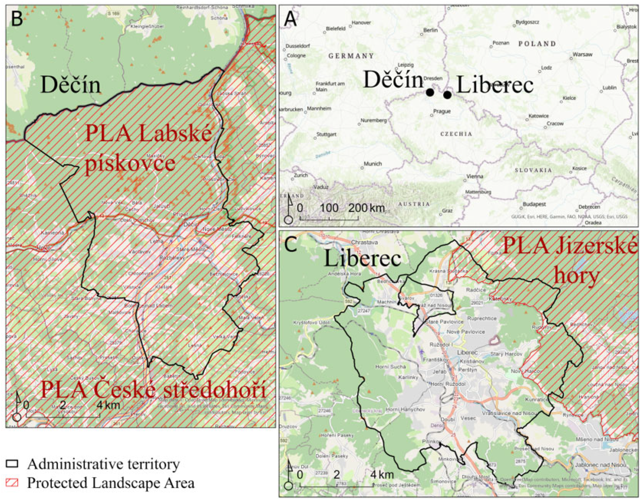
2.1. Location

The analysis was carried out for two cities in the northern part of the Czech Republic, Liberec and Děčín. Despite their rather industrial character, they have a large proportion of green areas and relatively high proportion of valuable habitats. They are situated on the border of protected landscape areas; the administrative territory of Liberec extends into the Jizera Mountains Protected Landscape Area in the northeastern part, while the Děčín administrative territory lies entirely in the nature protection regime, with the northern part in the Labské Pískovce Protected Landscape Area and the southern part in the České Středohoří Protected Landscape Area (Figure 1).
The two cities have a similar administrative territory, but they differ significantly in the number of inhabitants, being more than double in Liberec, which also has higher population growth. The geomorphological conditions are also different; Liberec is situated in a depression surrounded by hills with many small, radially oriented watercourses, while Děčín is situated in a narrow valley carved into the sandstone rock by the Elbe River and the Jílovský Brook, with the southeastern part of the valley merging into a wider floodplain with the Ploučnice tributary, surrounded by a hilly landscape. The detailed characteristics are described in Table 1.
Table 1. Characteristics of two administrative territories—Liberec and Děčín.
Name of the Administrative Territory Liberec Děčín
Area (km2) 106.1117.7
Elevation min–max (m a.s.l.) 296–1012115–708
Elevation mean (m a.s.l.) 469331
Predominant geological subsoil Granite, silt, marbleSandstone, impure carbonate sedimentary rock, basanite
Predominant soil types Cambisols, Leptosols, Podzols, Stagnosols, and Retisols Podzols, Cambisols, Leptosols, Stagnosols, and Luvisols
Annual average daily temperature (°C) 7.48.2
Annual average total precipitation (mm·year−1) 890640
CORINE LC (class level 1) 2018
(%)
Artificial surfaces31.512.5
Agricultural areas 27.421.7
Forest and seminatural areas41.264
Water bodies01.8
Number of citizens (1 January 2021)104,26147,951
Data sources: Czech Geological Survey [78,79]; Czech Hydrometeorological Institute [80,81]; Czech Statistical Office [82,83]; European Environment Agency [84].
Figure 1. (A) Location of Liberec and Děčín, Basemap: World Hillshade [85], World Topographic Map [86]; (B,C) administrative territory of Děčín and Liberec and protected landscape areas [87], Open Street map [88].
Applsci 13 05759 g001

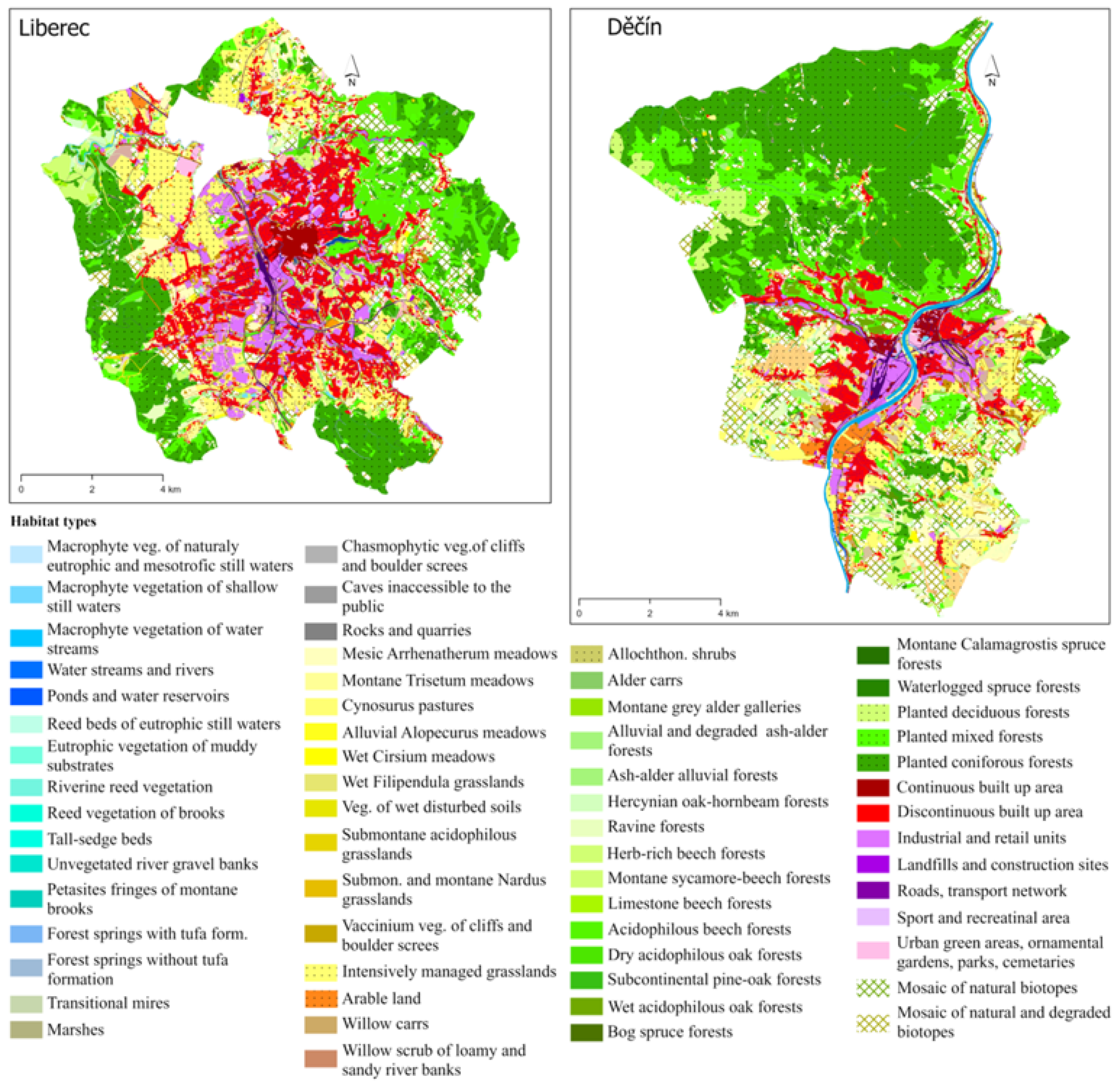
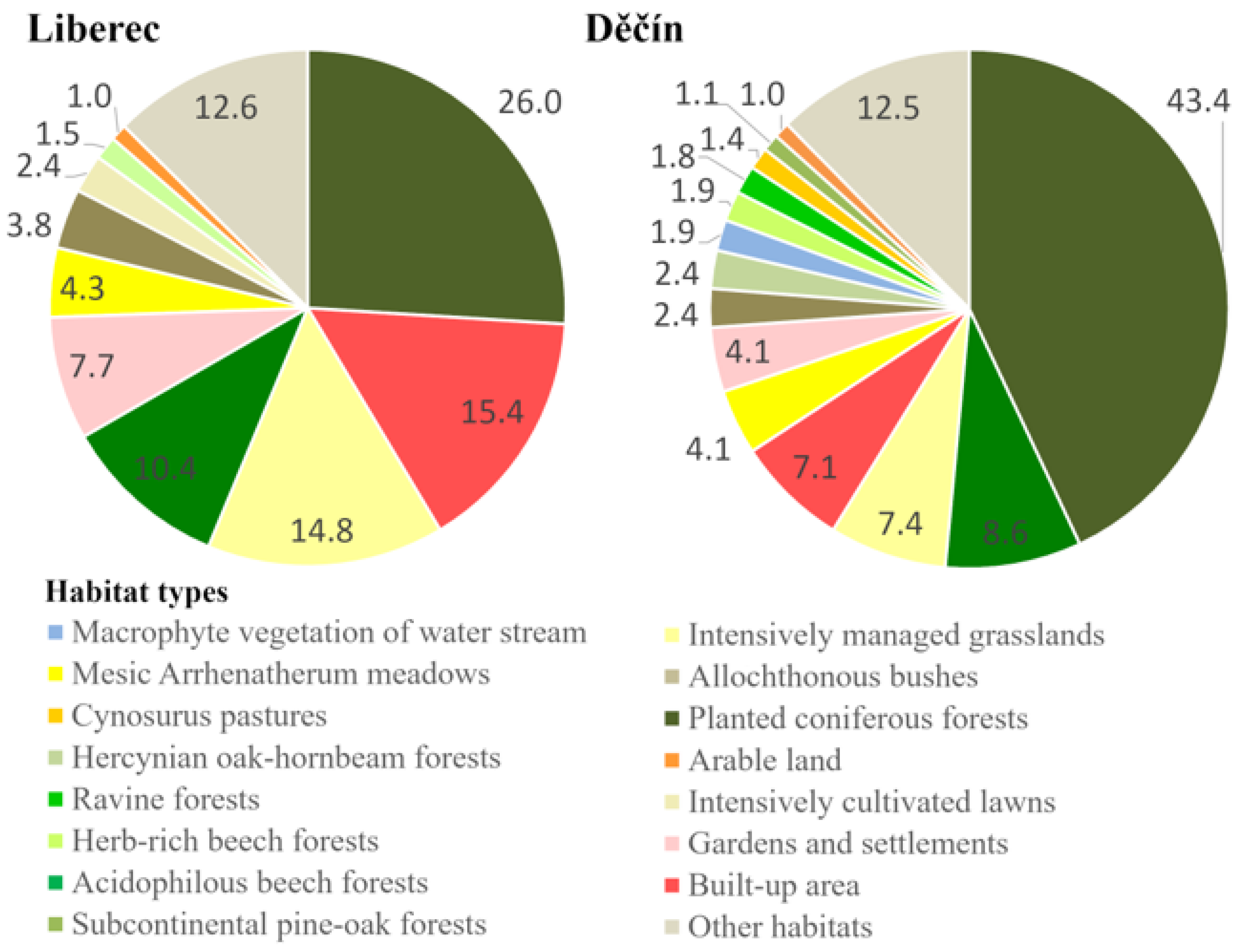
2.2. Map Data and Habitat Types

As a map base for this study, we used a detailed habitat layer that was created by combining two map layers: (i) the modified consolidated layer of ecosystems (© CzechGlobe © NCA CR, 2013) which distinguishes 41 categories with a mapping grain close to that of field mapping [89], and (ii) the habitat mapping layer [89], based on a detailed mapping of plant communities in the field for the purpose of mapping natural and near-natural habitats across the Czech Republic [90]. For more information about composition of the detailed habitat layer, see ref. [91]. The final map was further specified using the latest aerial photographs where necessary. All mapped habitats were expressed as 138 natural and near-natural habitats, according to Catalog of habitats in the Czech Republic [90], and 38 degraded habitats, according to Seják [36]. Map layers were created and edited in GIS using ArcMap 10.2.1 (see Figure 2).

2.3. Assessment of EFs Performance Indicating Habitat Capacity to Provide ESs

We opted for an assessment based on biophysical values using the quantification of biotic and abiotic configurations related to their capacity of ESs provision [18]. For assessment of regulation services, biophysical values are more suitable [20] and can combine measurable habitat patterns with inherent ecosystem functions and services [24]. In the administrative territories studied, the assessment of the degree of performance of ecosystem functions was used as an indicator of the capacity to provide the corresponding ecosystem services according to the ”ecosystem service cascade” of Potschin and Haines-Young [8]. The capacity of three key ecosystem services was assessed: provision of habitat/biodiversity, climate regulation at the local level, and climate regulation at the regional level. Habitat/biodiversity provision was assessed using habitat-level biodiversity and habitat connectivity at the landscape level, which allows an assessment of relationships between habitats. Climate regulation at the local scale was represented by an estimation of evapotranspiration, which is often used indicator in various urban ESs assessment studies (see ref. [22,49,50,51,92,93]). Climate regulation at the regional scale was assessed using the carbon production indicator. As suggested in the recent IPBES document [94], ecosystem uptake of greenhouse gasses is an appropriate indicator of climate regulation services; carbon storage was also used by ref. [14,16], while carbon sequestration or carbon production was used by ref. [10,11,13,95]. Values for the performance of individual ecosystem functions were assigned to the habitat types (for habitat-level biodiversity) or their functional groups (for evapotranspiration and carbon production) in the study area (lookup table approach) to produce a map of ecosystem functions. Habitat connectivity was assessed by analyzing the distances and spatial arrangement of natural and near-natural habitats.

2.3.1. Biodiversity Assessment at Habitat Level

The assessment was carried out using the habitat valuation method (HVM), a systematic method for establishing a list of national habitat types, classifying them according to their plant composition, and assessing their habitat provision value on the basis of an expert valuation of eight ecological criteria [36,96]. Habitats from this list of national habitat types for the Czech Republic were categorized according to their naturalness: natural and near-natural habitat types identified in the habitat mapping level (© NCA CR, 2015) and described in the Catalog of Habitats of the Czech Republic [90], as well as degraded habitat types divided into three naturalness levels (distant natural, unnatural, and human-made habitat groups) defined for the purposes of the HVM method [36,91,97]. Each habitat type was assigned a habitat provision value. A detailed description of the habitat classification method can be found in [98]; the list of habitat types and their point values are provided in Table S1 (Supplementary Materials).

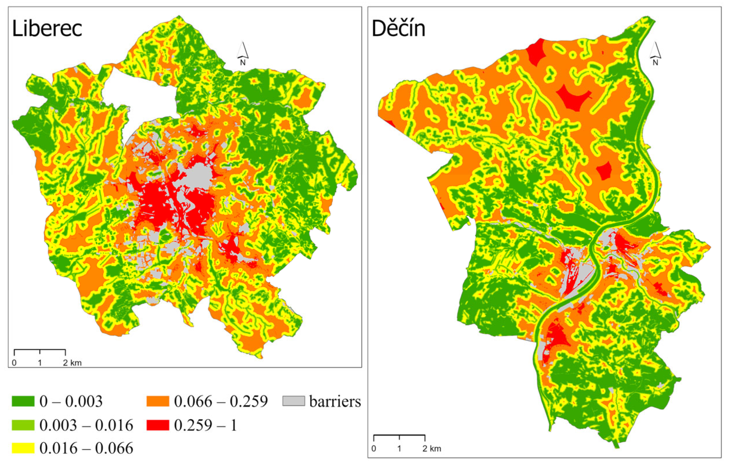
2.3.2. Habitat Connectivity Assessment at the Landscape Level

The modified distance to nature method, introduced by Rüdisser [38], was used as an indicator of connectivity at the landscape level. It assesses the distribution of valuable habitats and the distance to the nearest valuable habitat in the landscape. The habitat types from the HVM method and their five levels of naturalness were used for the analysis: the two best degrees of naturalness (natural and near-natural) for identification of valuable habitats, and the three remaining levels of degraded habitat types (distant natural, unnatural, and human) for resistance of habitats, forming a matrix for the dispersal of organisms. The Euclidean distance to the closest natural or near-natural habitat patch, multiplied by resistance values of the matrix, was calculated and expressed in the form of a continuous raster map, on the basis of which the mean values for reporting units were estimated. Values were normalized and scaled along a range from zero (no distance) to one (habitat completely far from natural habitat). For a more detailed description of the method, see [38]. To adapt the original method for use in urban landscapes, it was modified to consider roads and contiguous built-up areas larger than 0.25 ha as a total barrier to organism dispersal.

2.3.3. Assessment of Evapotranspiration

The method was developed in 2007–2009 by Seják [97,99]. It classifies the vegetation according to the annual transpiration. Transpiration assessments were conducted for 22 functional groups of habitats, into which the 193 HVM habitat types were grouped. For these groups, an expert estimate of average annual evapotranspiration was made, based partly on field measurements [99] and partly on findings and results from the work of the Botanical Institute of the Czech Academy of Sciences and others [100,101,102]. The functional groups of habitats and their estimated values of evapotranspiration are listed in Table 2.

2.3.4. Assessment of Carbon Production

The net annual production of above- and belowground biomass, i.e., the amount of dry matter in kg per m2 per year, was determined for the same functional groups as for evapotranspiration. These values were transferred from available literature sources, and repeated biomass sampling was carried out within the Czech Carbo project (see, e.g., ref. [103]). The detailed method was published in refs. [97,99,103]. The main functional groups of habitats and their estimated values of carbon production are presented in Table 2.

2.4. Parametrization and Relative Comparison of Values

In order to be able to assess and compare the relative performance of ecosystem functions, the values were parametrized into a uniform scale using Equation (1).
yi* = (yi − ymin)/(ymax − ymin),
where yi* is the parameterized value of the selected EFs, yi is the value of the selected EFs in relevant units, ymax is the maximal value of the selected EFs in relevant units, and ymin is the minimal value of the selected EFs in relevant units.
The three assessed EFs (biodiversity expressed by HVM, evapotranspiration, and carbon production) were merged into a single aggregated EFs performance by an average of the three parameterized values.

2.5. Assessment of Urban–Rural Gradient of EFs

We distinguished several levels of urban intensity: (i) the urban core, characterized by continuous development; (ii) the suburban area, where discontinuous development predominates, sometimes interspersed with other habitat types; (iii) the peri-urban area, which is an interface between the rural and the urban space, where there is an even smaller proportion of built-up areas; (iv) adjacent rural landscapes.
The spatial analysis of the urban–rural gradient of assessed ecosystem function was carried out using the buffer gradient analysis method, which is based on a series of equidistant buffer zones established starting from a circle in the urban core. The city center was defined as the geometric center (centroid) of the polygon of urban core area, which is identical to the historical city center. In Liberec, it was possible to identify only one centroid. In Děčín, due to the historical development that took place on both banks of the Elbe River, it was necessary to identify two focal points. A concentric buffer with 0.5 km intervals was created around the urban core area. In each ring section, the values of individual EFs were calculated.
Since Děčín does not have a typical city center, and the built-up areas are located in a narrow strip along the river, the gradient analysis was also carried out between the river and the outer landscape. A buffer of 0.5 km was created around the part of the Elbe (in Děčín) and the Neisse (in Liberec) to form the central river polygon. Equidistant buffer zones with a distance of 0.5 km were established around these river polygons. In each section, the values of individual EFs were calculated.
Spatial data analysis and map outputs were processed in the ArcGIS environment (ArcGIS Desktop 10.7.1 ESRI, 2019 and ArcGIS Pro 2.8.0 ESRI, 2021).

3. Results and Discussion

3.1. Results and Discussion of Method Application

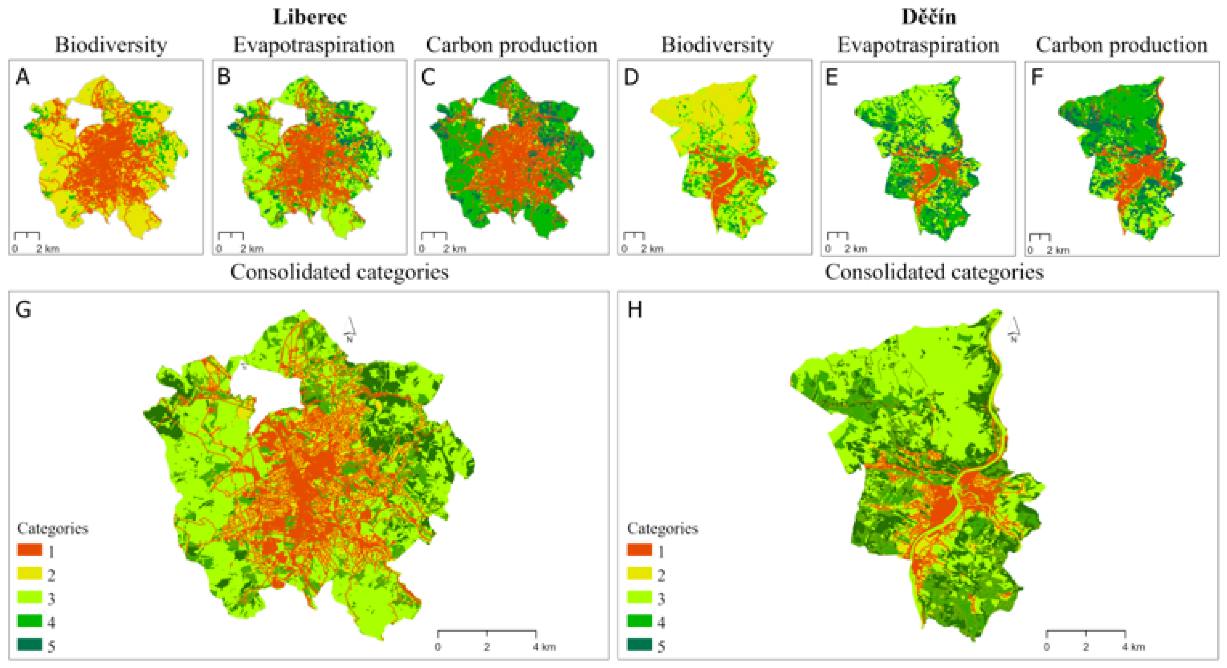
3.1.1. Values of EFs in Liberec and Děčín

Layers of habitats and their EFs, biodiversity (habitat assessment and structural connectivity), evapotranspiration, and annual carbon production were prepared for the administrative territories of Liberec and Děčín. The representation of habitat types, for which the ecosystem functions were quantified, is shown in Figure 3. Only habitats with more than 1% of the area are shown in the graph.
An overview of the results for the entire administrative territory of Liberec and Děčín is given in Table 3.
The average biodiversity score (HVM) was 19 points·m−2 in Liberec and 23 points·m−2 in Děčín. This is 2.15% (in Liberec) and 23.7% (in Děčín) more than the average HVM score for the Czech Republic, which is 18.6 points·m−2 [99]. Connectivity has extremely low values in the urban core area, which is considered almost entirely a barrier, and low values in the suburban area, especially in Liberec, where urban development is greater. According to Rüdisser [38], good connectivity corresponds to values up to 0.06, expressed on the map (Figure 4) by green and yellow color, covering 61% of the administrative territory in Liberec and 66% in Děčín. In Liberec, the good connectivity tends to be situated near the borders of administrative territory, especially in the area that is part of the PLA Jizerské hory. In Děčín, connectivity was good, especially in the peri-urban area of the city and on the steep slopes near the river Elbe, most of which are covered with natural and near-natural habitats. In the areas close to the northern boundary of the administrative territory, connectivity decreased due to large areas covered by planted, low-diversity spruce forests. The graphical representation of connectivity shows corridors that consist of well-connected habitats. Both cities contain watercourses that are indispensable natural corridors for the movement of organisms and for the flow of materials and energy. Supporting and further connecting these corridors, especially in areas with lower connectivity, is a land-use planning task to create a functioning blue and green infrastructure. This connectivity has positive impacts, especially on biodiversity [104].
For connectivity planning, the selection of appropriate data is crucial. As already stated, standard land-use and land-cover data are not detailed enough for the urban administrative territory level [32], and remote sensing data, which have recently become widely available, may be sufficient for carbon storage and possibly for estimating evapotranspiration but do not contain sufficient information on species and habitats for biodiversity assessment (although there is ongoing progress in this area; see ref. [105]). Therefore, the use of more detailed habitat mapping data using the lookup table approach seems to be the simplest way to obtain results on the distribution of EFs and biodiversity in urban administrative territories.
The average value of evapotranspiration was 463 L·m−2·year−1 in Liberec and 502 L·m−2·year−1 in Děčín. Comparing these values with the average value for the Czech Republic, 421.4 L·m−2·year−1 published by Seják [99], they are higher by 9.9% and 19.1%, respectively. The amount of carbon production was 5.3 t·ha−1·year−1 in Liberec and 5.9 t·ha−1·year−1 in Děčín, which exceeds the average value for the Czech Republic of 5.1 t·ha−1·year−1 published by Seják [99] by 3.9% and 15.7%, respectively. The values of carbon production also significantly exceed the published values of average carbon sequestration in urban areas in various cities in Asia and North America, which ranged from 2.16 to 3.06 t·ha−1·year−1 [64,106,107]. The results clearly show that EFs related to climate change mitigation can be performed better in very heterogeneous urban administrative territories with urban forests, parks, and other green spaces than in common landscapes. In particular, peri-urban areas of cities located near (or within) protected landscape areas, as in the case of Liberec and Děčín, can have a high value of EFs.

3.1.2. Comparison of Liberec and Děčín

Although Liberec and Děčín are comparable in terms of area, ecosystem function values differ substantially. Habitat-level biodiversity, expressed in HVM values, was almost 33% higher in Děčín than in Liberec, as was the average connectivity value, which was 22% higher. Annual carbon production was 23% higher and evapotranspiration was 20% higher than in Liberec. These differences can be attributed mainly to the stronger population growth and the related faster development of the built-up area in Liberec, while, in Děčín, the number of inhabitants (similar population to 100 years ago, Czech Statistical Office, 2006) and the development of the city have more or less stagnated; consequently, the current built-up area in Liberec is twice as large as in Děčín. Accordingly, the share of forests in Liberec is lower (only 24%), while, in Děčín, forests cover almost half of the administrative territory. However, the protection regime probably had a dominant influence on the fact that ecosystem functions in the territory of Děčín reached significantly higher values than in Liberec, as most of the cadaster of Děčín falls within two PLAs, while, in the case of Liberec, only a small percentage of the administrative territory belongs to the PLA.

3.1.3. Relative Comparison of Values of Individual EFs

A comparison of the relative parameterized values of the ecosystem functions assessed (see Figure 5A–F) shows that the lowest values apply to habitat-level biodiversity (HVM), especially in the urban core and suburban area and, in the case of Děčín, also near the northern boundary, where there are large stands of planted spruce forests. The other two functions, evapotranspiration and especially production, have relatively higher values and, unlike biodiversity, are also located to a limited extent in the suburban area.
The disparate results (especially lower biodiversity compared to other EFs) are consistent with findings that certain habitat features are important for maintaining biodiversity but are not as critical for maintaining other ecosystem functions. Species diversity in urban vegetation depends on diverse vegetation structure and vertical complexity [108,109], the naturalness of the habitat [110], and eventually, the proportion of native trees [111] and the intensity of management [29]. Some of these characteristics are not as important for the other two functions (carbon production and evapotranspiration), as these depend mainly on the vegetation biomass [112] and LAI values [54], as well as, in the case of evapotranspiration, physiological characteristics such as tree-level transpiration [113]. These results suggest that certain habitats with average and sometimes rather low biodiversity values (mainly planted spruce forests but also urban parks and other urban green spaces) can, due to their high biomass, provide ecosystem services that contribute notably to cooling of the urban environment through evapotranspiration and to mitigating climate change through carbon sequestration.
Merging of the three EFs into one value (Figure 5G,H) shows the location of area of the best EFs performance. In Liberec, they are situated mostly near the border of the administrative territory, especially where the PLA is defined; however, there are some habitats of relatively high EFs performance situated in the suburban area. In Děčín, the peri-urban area has a very high EFs performance. On the contrary, the worst values of EFs were found in the urban core areas, which are almost devoid of vegetation, and in the suburban areas, where discontinuous development predominates.

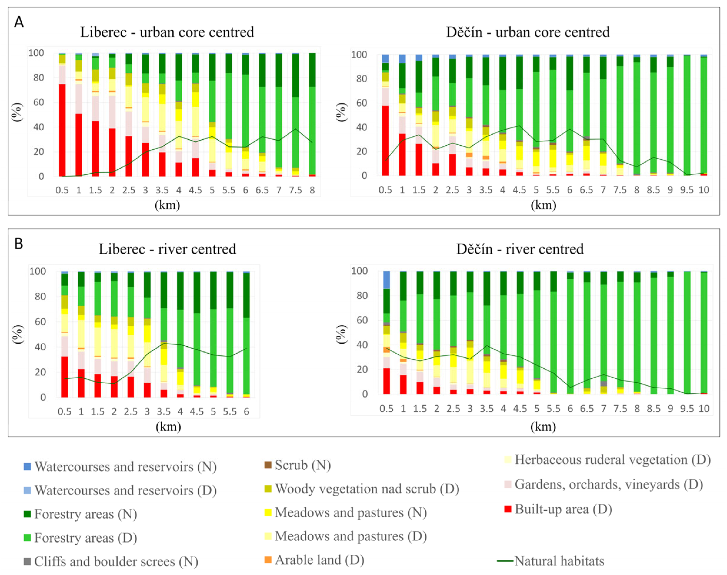
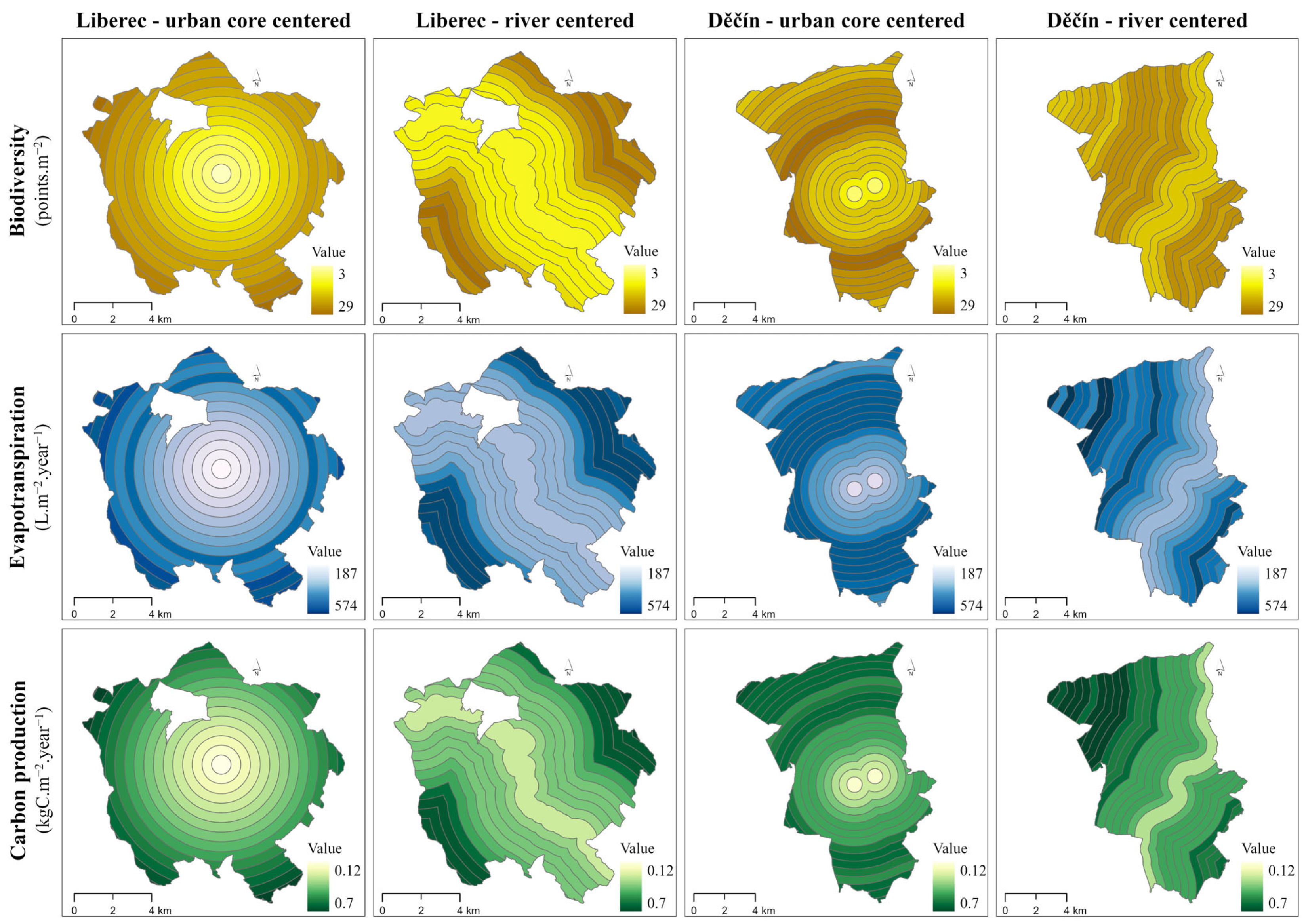
3.1.4. The Urban–Rural Gradient

The urban–rural gradient shows how much the composition of habitats differs (see Figure 6) and how the values of EFs change depending on the distance (a) from the center in the case of a city with typical urban core, or (b) from the river in the case of a city with development situated around the river (see Figure 7).
In the case of Liberec, it is noticeable that the values of EFs increase relatively gradually with increasing distance from the center. Only evapotranspiration increases sharply at a distance of 5 km, before decreasing and starting to increase again; this may be due to the relatively large area of alluvial and deciduous forests, as well as wet meadows in this area. The prevailing gradual pattern of EFs increase is also supported by geomorphological conditions. Liberec lies in a valley whose slopes gradually rise to the foot of the Jizera Mountains in the northeast and the Ještěd Mountain in the southwest; the city grows on all sides relatively evenly. In Liberec, the center with very low values of all EFs spreads across a diameter of about 5–6 km; in Děčín, this area with low EFs extends cross a diameter of only 2–3 km, corresponding to the different size of urbanized area. In Děčín, the gradient is very uneven, as values increase at much shorter distances from the center but decrease again when reaching 5 km from the center (in the case of HVM value and carbon production) or 8 km in the case of evapotranspiration caused by river Elbe influence and high share of deciduous forests. This situation is supported by a particular geomorphology. At a certain distance from the urban core (and from the river), there are steep slopes carved by the river in the sandstone rock, which are not suitable for urban or agricultural use and are, therefore, mainly covered by natural and near-natural habitats. The plateau that continues above these slopes is dominated by planted spruce forests; thus, the biodiversity value decreases at greater distances. A similar trend in urban–rural gradient was described by Baró [17] for EFs/ESs in Barcelona, where it was found that areas closer to the city had higher values than the surrounding agricultural landscape. From Figure 2, it is apparent that, especially in the case of Děčín, the peri-urban area is covered by diverse habitats with relatively high proportion of natural and near-natural habitats.
The highly urbanized area is, especially in Děčín, concentrated around a large watercourse and creates a narrow strip of development in the valley along the river. To visualize the specific gradient, a buffer around the river was created, revealing that, instead of forming blue and green infrastructure of high habitat quality, areas around watercourses are of the lowest value concerning studied EFs. A suitable strategy would be the development of blue and green corridors for pedestrian and animal movement, biodiversity, and ecosystem service support [75].

3.2. Discussion of the Method Choice

We chose the biophysical (also called indicator-based [114]) method to avoid underestimation, to which the use of sociocultural methods (according to ref. [20]) could lead. Studies comparing biophysical and sociocultural values to assess local climate change mitigation services are rare (e.g., ref. [115]). Biophysical values quantify biotic and abiotic configurations related to the provision of ESs [18]. For our three selected ESs, we sought suitable indicators that have been recommended in official reports or used in a number of other studies (see Section 1.3). From the range of suitable indicators, we selected those suitable for the scale of the entire urban administrative territory and in the lookup table approach, which we preferred because of its ease of use in practice. The methods and data used for their quantification were based on the results of previous projects of the Czech Ministry of Life Environment (Czech Carbo, Czech Terra, habitat valuation of the Czech Republic, and valuation of ecosystem functions and services of the Czech Republic) and the Interreg project Bidelin, in which the authors of this paper participated.
Because the urban administrative territory consists of clearly definable segments to which the values and approaches apply, the performance of ecosystem functions can be calculated for each segment. Although most lookup table methods use land-cover data as a basis [116], in most cases, these data are not detailed enough to assess EFs at the urban administrative territory level [32]. In this case, the European Commission suggests using maps created by combining land-cover maps with habitat databases [20]; we used this principle to create a detailed habitat layer and augmented it with other data sources, some of which were results from the Czech case study involved in the ESMERALDA project [117] to make it more precise. To capture the influence of a higher hierarchical level of landscape structure and its complexity, we calculated the connectivity indicator, which indicates the distance (within the urban area structure) to the nearest natural habitat within which the EFs are performed without negative human influence. Ecosystem function values are assigned to individual habitat types or their groups, which makes the method easily applicable and allows transferring the values to other European countries with similar climatic conditions (and, thus, habitat types).

4. Conclusions

We presented a method for assessing three EFs of urban and peri-urban habitats (biodiversity, evapotranspiration, and carbon production) indicating their capacity to provide associated ESs (habitat provision and climate regulation at local and regional scales). The simplicity of application of the lookup table approach based on values associated with habitat types makes it suitable not only for urban areas but also for the adjacent rural landscape and enables analysis of the urban–rural gradient of EFs values. The values assigned to habitat types can be transferred to other European countries with similar climatic conditions and, thus, habitat types.
The application of the method to the administrative territories of two cities, Liberec and Děčín, revealed high performance of EFs, which was even higher than the average for the whole country. Urban and suburban areas had the lowest values, but the peri-urban areas had surprisingly high values for habitat connectivity and other EFs, especially in Děčín, where the special conditions led to a concentration of valuable habitats in this area. The urban–rural analysis also supported this result, showing higher values for biodiversity and connectivity in peri-urban areas than in the adjacent rural landscape. The lowest values of the three studied ESs were obtained for habitat-level biodiversity, especially in the urban core and suburbs and near the boundary of the administrative territory. This indicates that many habitat types typical of urban and peri-urban areas may perform climate-regulating functions relatively well, but do not support biodiversity to the same extent. Therefore, promoting biodiversity should be a priority in urban adaptation plans.
This method can serve as a useful tool to quickly identify valuable urban habitats (strong EFs providers) and advocate for their protection or, on the contrary, identify places with low values of EFs. In particular, low values of evapotranspiration in the central area of cities and the low connectivity of valuable habitats are situations that should be prioritized and sorted in urban adaptation strategies toward global climate change.

Supplementary Materials

The following supporting information can be downloaded at https://www.mdpi.com/article/10.3390/app13095759/s1, Table S1. Habitat types and their relative point values according to ref. [36].

Author Contributions

Conceptualization, M.P., R.V., and P.C.; methodology, M.P.; software, V.P.; validation, L.Š., J.P., and P.C.; formal analysis R.V.; investigation V.P. and R.V.; resources, A.M.A.A.; data curation, V.P. and R.V.; writing—original draft preparation, M.P.; writing—review & editing, P.C., R.V., L.Š., J.P., and O.C.; visualization, R.V.; supervision, P.C.; project administration, P.C.; funding acquisition, P.C. All authors read and agreed to the published version of the manuscript.

Funding

This research was funded by the EU project BIDELIN “The values of ecosystem services, biodiversity, and green–blue infrastructure in cities using the examples of Dresden, Liberec, and Děčín” in the framework of the Interreg V-A 2014-2020 Saxony–Czech Republic and by the institutional project of the Global Change Research Institute of the Czech Academy of Sciences.

Institutional Review Board Statement

Not applicable.

Informed Consent Statement

Not applicable.

Data Availability Statement

The data are available from the authors upon request.

Acknowledgments

This work was supported by the EU project BIDELIN and by the Global Change Research Institute of the Czech Academy of Sciences.

Conflicts of Interest

The authors declare no conflict of interest.

Abbreviations

CRCzech Republic
EFsEcosystem function
ESsEcosystem services
HVMHabitat valuation method
LAILeaf area index
NCA CRNature Conservation Agency of the Czech Republic
NDVINormalized difference vegetation index
PLAProtected landscape area
TEEBThe Economics of Ecosystems and Biodiversity

References

  1. Mexia, T.; Vieira, J.; Príncipe, A.; Anjos, A.; Silva, P.; Lopes, N.; Freitas, C.; Santos-Reis, M.; Correia, O.; Branquinho, C.; et al. Ecosystem Services: Urban Parks under a Magnifying Glass. Environ. Res. 2018, 160, 469–478. [Google Scholar] [CrossRef] [PubMed]
  2. Richards, D.R.; Belcher, R.N. Global Changes in Urban Vegetation Cover. Remote Sens. 2019, 12, 23. [Google Scholar] [CrossRef]
  3. Gill, S.E.; Handley, J.F.; Ennos, A.R.; Pauleit, S. Adapting Cities for Climate Change: The Role of the Green Infrastructure. Built Environ. 2007, 33, 115–133. [Google Scholar] [CrossRef]
  4. Pereira, H.M.; Leadley, P.W.; Proença, V.; Alkemade, R.; Scharlemann, J.P.W.; Fernandez-Manjarrés, J.F.; Araújo, M.B.; Balvanera, P.; Biggs, R.; Cheung, W.W.L.; et al. Scenarios for Global Biodiversity in the 21st Century. Science 2010, 330, 1496–1501. [Google Scholar] [CrossRef]
  5. Benedict, M.A.; McMahon, E.T. Green Infrastructure: Smart Conservation for the 21st Century. Renew. Resour. J. 2002, 20, 12–17. [Google Scholar]
  6. TEEB The Economics of Ecosystems and Biodiversity: TEEB Manual for Cities—Ecosystem Services in Urban Management. 2011. Available online: www.teebweb.org (accessed on 3 December 2022).
  7. Villamagna, A.M.; Angermeier, P.L.; Bennett, E.M. Capacity, Pressure, Demand, and Flow: A Conceptual Framework for Analyzing Ecosystem Service Provision and Delivery. Ecol. Complex. 2013, 15, 114–121. [Google Scholar] [CrossRef]
  8. Potschin, M.B.; Haines-Young, R.H. Ecosystem Services: Exploring a Geographical Perspective. Prog. Phys. Geogr. Earth Environ. 2011, 35, 575–594. [Google Scholar] [CrossRef]
  9. Elmqvist, T.; Setälä, H.; Handel, S.; Van Der Ploeg, S.; Aronson, J.; Blignaut, J.; Gómez-Baggethun, E.; Nowak, D.; Kronenberg, J.; De Groot, R. Benefits of Restoring Ecosystem Services in Urban Areas. Curr. Opin. Environ. Sustain. 2015, 14, 101–108. [Google Scholar] [CrossRef]
  10. Gómez-Baggethun, E.; Barton, D.N. Classifying and Valuing Ecosystem Services for Urban Planning. Ecol. Econ. 2013, 86, 235–245. [Google Scholar] [CrossRef]
  11. Li, S.; Liang, W.; Fu, B.; Lü, Y.; Fu, S.; Wang, S.; Su, H. Vegetation Changes in Recent Large-Scale Ecological Restoration Projects and Subsequent Impact on Water Resources in China’s Loess Plateau. Sci. Total Environ. 2016, 569–570, 1032–1039. [Google Scholar] [CrossRef]
  12. Rovai, M.; Zetti, I.; Lucchesi, F.; Rossi, M.; Andreoli, M. Peri-Urban Open Spaces and Sustainable Urban Development Between Value and Consumption. In Values and Functions for Future Cities; Mondini, G., Oppio, A., Stanghellini, S., Bottero, M., Abastante, F., Eds.; Green Energy and Technology; Springer International Publishing: Cham, Switzerland, 2020; pp. 249–265. [Google Scholar]
  13. Salata, S.; Giaimo, C.; Alberto Barbieri, C.; Garnero, G. The Utilization of Ecosystem Services Mapping in Land Use Planning: The Experience of LIFE SAM4CP Project. J. Environ. Plan. Manage. 2020, 63, 523–545. [Google Scholar] [CrossRef]
  14. Salizzoni, E.; Allocco, M.; Murgese, D.; Quaglio, G. From Ecosystem Service Evaluation to Landscape Design: The Project of a Rural Peri-Urban Park in Chieri (Italy). In Values and Functions for Future Cities; Mondini, G., Oppio, A., Stanghellini, S., Bottero, M., Abastante, F., Eds.; Green Energy and Technology; Springer International Publishing: Cham, Switzerland, 2020; pp. 267–283. [Google Scholar] [CrossRef]
  15. Marando, F.; Salvatori, E.; Sebastiani, A.; Fusaro, L.; Manes, F. Regulating Ecosystem Services and Green Infrastructure: Assessment of Urban Heat Island Effect Mitigation in the Municipality of Rome, Italy. Ecol. Modell. 2019, 392, 92–102. [Google Scholar] [CrossRef]
  16. Davies, Z.G.; Edmondson, J.L.; Heinemeyer, A.; Leake, J.R.; Gaston, K.J. Mapping an Urban Ecosystem Service: Quantifying above-Ground Carbon Storage at a City-Wide Scale: Urban above-Ground Carbon Storage. J. Appl. Ecol. 2011, 48, 1125–1134. [Google Scholar] [CrossRef]
  17. Baró, F.; Gómez-Baggethun, E.; Haase, D. Ecosystem Service Bundles along the Urban-Rural Gradient: Insights for Landscape Planning and Management. Ecosyst. Serv. 2017, 24, 147–159. [Google Scholar] [CrossRef]
  18. Vihervaara, P.; Mononen, L.; Nedkov, S.; Viinikka, A. Biophysical Mapping and Assessment Methods for Ecosystem Services; Deliverable D3.3 EU Horizon 2020 ESMERALDA Project, Grant Agreement No. 642007; European Commission: Luxembourg, 2018. [Google Scholar]
  19. Chan, K.M.A.; Guerry, A.D.; Balvanera, P.; Klain, S.; Satterfield, T.; Basurto, X.; Bostrom, A.; Chuenpagdee, R.; Gould, R.; Halpern, B.S.; et al. Where Are Cultural and Social in Ecosystem Services? A Framework for Constructive Engagement. BioScience 2012, 62, 744–756. [Google Scholar] [CrossRef]
  20. European Commission. EU Guidance on Integrating Ecosystems and Their Services into Decision-Making; European Commission: Brussels, Belgium, 2019; Available online: https://ec.europa.eu/environment/nature/ecosystems/pdf/SWD_2019_305_F1_STAFF_WORKING_PAPER_EN_V2_P1_1042629.PDF (accessed on 19 April 2023).
  21. Dobbs, C.; Escobedo, F.J.; Zipperer, W.C. A Framework for Developing Urban Forest Ecosystem Services and Goods Indicators. Landsc. Urban Plan. 2011, 99, 196–206. [Google Scholar] [CrossRef]
  22. Larondelle, N.; Haase, D. Urban Ecosystem Services Assessment along a Rural–Urban Gradient: A Cross-Analysis of European Cities. Ecol. Indicat. 2013, 29, 179–190. [Google Scholar] [CrossRef]
  23. OECD (Ed.) Environmental indicators: 2001 towards sustainable development. In Environment; OECD: Paris, France, 2001. [Google Scholar]
  24. Niemi, G.J.; McDonald, M.E. Application of Ecological Indicators. Annu. Rev. Ecol. Evol. Syst. 2004, 35, 89–111. [Google Scholar] [CrossRef]
  25. Bellard, C.; Bertelsmeier, C.; Leadley, P.; Thuiller, W.; Courchamp, F. Impacts of Climate Change on the Future of Biodiversity: Biodiversity and Climate Change. Ecol. Lett. 2012, 15, 365–377. [Google Scholar] [CrossRef] [PubMed]
  26. Lavorel, S.; Colloff, M.J.; Mcintyre, S.; Doherty, M.D.; Murphy, H.T.; Metcalfe, D.J.; Dunlop, M.; Williams, R.J.; Wise, R.M.; Williams, K.J. Ecological Mechanisms Underpinning Climate Adaptation Services. Glob. Change Biol. 2015, 21, 12–31. [Google Scholar] [CrossRef] [PubMed]
  27. Higgins, P.A.T. Biodiversity Loss under Existing Land Use and Climate Change: An Illustration Using Northern South America. Glob. Ecol. Biogeogr. 2007, 16, 197–204. [Google Scholar] [CrossRef]
  28. Aronson, M.F.J.; La Sorte, F.A.; Nilon, C.H.; Katti, M.; Goddard, M.A.; Lepczyk, C.A.; Warren, P.S.; Williams, N.S.G.; Cilliers, S.; Clarkson, B.; et al. A Global Analysis of the Impacts of Urbanization on Bird and Plant Diversity Reveals Key Anthropogenic Drivers. Proc. R. Soc. B. 2014, 281, 20133330. [Google Scholar] [CrossRef] [PubMed]
  29. Lepczyk, C.A.; Aronson, M.F.J.; Evans, K.L.; Goddard, M.A.; Lerman, S.B.; MacIvor, J.S. Biodiversity in the City: Fundamental Questions for Understanding the Ecology of Urban Green Spaces for Biodiversity Conservation. BioScience 2017, 67, 799–807. [Google Scholar] [CrossRef]
  30. Ives, C.D.; Lentini, P.E.; Threlfall, C.G.; Ikin, K.; Shanahan, D.F.; Garrard, G.E.; Bekessy, S.A.; Fuller, R.A.; Mumaw, L.; Rayner, L.; et al. Cities Are Hotspots for Threatened Species: The Importance of Cities for Threatened Species. Glob. Ecol. Biogeogr. 2016, 25, 117–126. [Google Scholar] [CrossRef]
  31. Kowarik, I. Novel Urban Ecosystems, Biodiversity, and Conservation. Environ. Pollut. 2011, 159, 1974–1983. [Google Scholar] [CrossRef]
  32. Jarvis, P.J.; Young, C.H. The mapping of urban habitat and its evaluation. In Urban Forum of the United Kingdom Man and the Biosphere Programme; University of Wolverhampton: Wolverhampton, UK, 2005. [Google Scholar]
  33. Hong, S.-K.; Song, I.-J.; Byun, B.; Yoo, S.; Nakagoshi, N. Applications of Biotope Mapping for Spatial Environmental Planning and Policy: Case Studies in Urban Ecosystems in Korea. Landsc. Ecol. Eng. 2005, 1, 101–112. [Google Scholar] [CrossRef]
  34. Weiers, S.; Bock, M.; Wissen, M.; Rossner, G. Mapping and Indicator Approaches for the Assessment of Habitats at Different Scales Using Remote Sensing and GIS Methods. Landsc. Urban Plan. 2004, 67, 43–65. [Google Scholar] [CrossRef]
  35. Kowarik, I.; von der Lippe, M. Plant Population Success across Urban Ecosystems: A Framework to Inform Biodiversity Conservation in Cities. J. Appl. Ecol. 2018, 55, 2354–2361. [Google Scholar] [CrossRef]
  36. Seják, J.; Cudlín, P.; Petříček, V.; Prokopová, M.; Cudlín, O.; Holcová, D.; Kaprová, K.; Melichar, J.; Škarková, P.; Žákovská, K.; et al. Metodika hodnocení biotopů AOPK ČR (6. verze). In Habitat Assessment Methodology NCA CR, 6th ed.; AOPK: Prague, Czech Republic, 2018; Available online: http://www.imalbes.cz/file/metodika_BVM.pdf (accessed on 12 December 2022).
  37. Schittko, C.; Bernard-Verdier, M.; Heger, T.; Buchholz, S.; Kowarik, I.; Lippe, M.; Seitz, B.; Joshi, J.; Jeschke, J.M. A Multidimensional Framework for Measuring Biotic Novelty: How Novel Is a Community? Glob. Change Biol. 2020, 26, 4401–4417. [Google Scholar] [CrossRef] [PubMed]
  38. Rüdisser, J.; Tasser, E.; Tappeiner, U. Distance to Nature—A New Biodiversity Relevant Environmental Indicator Set at the Landscape Level. Ecol. Indicat. 2012, 15, 208–216. [Google Scholar] [CrossRef]
  39. Tischendorf, L.; Fahrig, L. On the Usage and Measurement of Landscape Connectivity. Oikos 2000, 90, 7–19. [Google Scholar] [CrossRef]
  40. Benayas, J.M.R.; Bullock, J.M.; Newton, A.C. Creating Woodland Islets to Reconcile Ecological Restoration, Conservation, and Agricultural Land Use. Front. Ecol. Environ. 2008, 6, 329–336. [Google Scholar] [CrossRef]
  41. Bergsten, A.; Galafassi, D.; Bodin, Ö. The Problem of Spatial Fit in Social-Ecological Systems: Detecting Mismatches between Ecological Connectivity and Land Management in an Urban Region. Ecol. Soc. 2014, 19, 22. [Google Scholar] [CrossRef]
  42. Hejkal, J.; Buttschardt, T.K.; Klaus, V.H. Connectivity of Public Urban Grasslands: Implications for Grassland Conservation and Restoration in Cities. Urban Ecosyst. 2017, 20, 511–519. [Google Scholar] [CrossRef]
  43. Ren, Y.; Deng, L.; Zuo, S.; Luo, Y.; Shao, G.; Wei, X.; Hua, L.; Yang, Y. Geographical Modeling of Spatial Interaction between Human Activity and Forest Connectivity in an Urban Landscape of Southeast China. Landsc. Ecol. 2014, 29, 1741–1758. [Google Scholar] [CrossRef]
  44. Lee, H.; Mayer, H.; Chen, L. Contribution of Trees and Grasslands to the Mitigation of Human Heat Stress in a Residential District of Freiburg, Southwest Germany. Landsc. Urban Plan. 2016, 148, 37–50. [Google Scholar] [CrossRef]
  45. Zölch, T.; Maderspacher, J.; Wamsler, C.; Pauleit, S. Using Green Infrastructure for Urban Climate-Proofing: An Evaluation of Heat Mitigation Measures at the Micro-Scale. Urban For. Urban Green. 2016, 20, 305–316. [Google Scholar] [CrossRef]
  46. Demuzere, M.; Orru, K.; Heidrich, O.; Olazabal, E.; Geneletti, D.; Orru, H.; Bhave, A.G.; Mittal, N.; Feliu, E.; Faehnle, M. Mitigating and Adapting to Climate Change: Multi-Functional and Multi-Scale Assessment of Green Urban Infrastructure. J. Environ. Manag. 2014, 146, 107–115. [Google Scholar] [CrossRef] [PubMed]
  47. Meili, N.; Manoli, G.; Burlando, P.; Carmeliet, J.; Chow, W.T.L.; Coutts, A.M.; Roth, M.; Velasco, E.; Vivoni, E.R.; Fatichi, S. Tree Effects on Urban Microclimate: Diurnal, Seasonal, and Climatic Temperature Differences Explained by Separating Radiation, Evapotranspiration, and Roughness Effects. Urban For. Urban Green. 2021, 58, 126970. [Google Scholar] [CrossRef]
  48. Rahman, M.A.; Moser, A.; Gold, A.; Rötzer, T.; Pauleit, S. Vertical Air Temperature Gradients under the Shade of Two Contrasting Urban Tree Species during Different Types of Summer Days. Sci. Total Environ. 2018, 633, 100–111. [Google Scholar] [CrossRef] [PubMed]
  49. Burkhard, B.; Kroll, F.; Nedkov, S.; Müller, F. Mapping Ecosystem Service Supply, Demand and Budgets. Ecol. Indicat. 2012, 21, 17–29. [Google Scholar] [CrossRef]
  50. Larondelle, N.; Haase, D.; Kabisch, N. Mapping the Diversity of Regulating Ecosystem Services in European Cities. Global Environ. Change 2014, 26, 119–129. [Google Scholar] [CrossRef]
  51. Schwarz, N.; Bauer, A.; Haase, D. Assessing Climate Impacts of Planning Policies—An Estimation for the Urban Region of Leipzig (Germany). Environ. Impact Assess. Rev. 2011, 31, 97–111. [Google Scholar] [CrossRef]
  52. Armson, D. The Effect of Trees and Grass on the Thermal and Hydrological Performance of an Urban Area. Ph.D. Thesis, The University of Manchester, Manchester, UK, 2012. [Google Scholar]
  53. Konarska, J.; Holmer, B.; Lindberg, F.; Thorsson, S. Influence of Vegetation and Building Geometry on the Spatial Variations of Air Temperature and Cooling Rates in a High-Latitude City: Spatial Variations of Air Temperature in a High Latitude City. Int. J. Climatol. 2016, 36, 2379–2395. [Google Scholar] [CrossRef]
  54. Rahman, M.A.; Moser, A.; Rötzer, T.; Pauleit, S. Within Canopy Temperature Differences and Cooling Ability of Tilia Cordata Trees Grown in Urban Conditions. Build. Environ. 2017, 114, 118–128. [Google Scholar] [CrossRef]
  55. Coccolo, S.; Kämpf, J.; Scartezzini, J.-L.; Pearlmutter, D. Outdoor Human Comfort and Thermal Stress: A Comprehensive Review on Models and Standards. Urban Climate 2016, 18, 33–57. [Google Scholar] [CrossRef]
  56. Bartesaghi-Koc, C.; Osmond, P.; Peters, A. Mapping and Classifying Green Infrastructure Typologies for Climate-Related Studies Based on Remote Sensing Data. Urban For. Urban Green. 2019, 37, 154–167. [Google Scholar] [CrossRef]
  57. Paschalis, A.; Chakraborty, T.; Fatichi, S.; Meili, N.; Manoli, G. Urban Forests as Main Regulator of the Evaporative Cooling Effect in Cities. AGU Adv. 2021, 2, e2020AV000303. [Google Scholar] [CrossRef]
  58. Hesslerová, P.; Pokorný, J.; Brom, J.; Rejšková-Procházková, A. Daily Dynamics of Radiation Surface Temperature of Different Land Cover Types in a Temperate Cultural Landscape: Consequences for the Local Climate. Ecol. Eng. 2013, 54, 145–154. [Google Scholar] [CrossRef]
  59. Farrugia, S.; Hudson, M.D.; McCulloch, L. An Evaluation of Flood Control and Urban Cooling Ecosystem Services Delivered by Urban Green Infrastructure. Int. J. Biodiv. Sci. Ecosyst. Serv. Manag. 2013, 9, 136–145. [Google Scholar] [CrossRef]
  60. Becker, G.; Richard, M. The Biotope Area Factor as an Ecological Parameter–Principles for Its Determination and Identification of the Target 1990. Available online: www.berlin.de›bffbiotopflaechenfaktor›auszug_bff_gutachten_1990_eng (accessed on 19 April 2023).
  61. Kruuse, A. GRaBS Expert Paper 6: The Green Space Factor and the Green Points System; Town and Country Planning Association: London, UK, 2011. [Google Scholar]
  62. Sharp, R.; Chaplin-Kramer, R.; Wood, S.A.; Guerry, A.; Tallis, H.T.; Ricketts, T.; Nelson, E.J.; Ennaanay, D.; Wolny, S.; Olwero, N.; et al. VEST 2.2.2 User’s Guide; The Natural Capital, Project; The Nature Conservancy, and World Wildllife Fund; Stanford University: Stanford, CA, USA; University of Minnesota: Minneapolis, MN, USA, 2011. [Google Scholar]
  63. Robinson, D. Implications of a Large Global Root Biomass for Carbon Sink Estimates and for Soil Carbon Dynamics. Proc. R. Soc. B 2007, 274, 2753–2759. [Google Scholar] [CrossRef] [PubMed]
  64. Nowak, D.J.; Greenfield, E.J.; Hoehn, R.E.; Lapoint, E. Carbon Storage and Sequestration by Trees in Urban and Community Areas of the United States. Environ. Pollut. 2013, 178, 229–236. [Google Scholar] [CrossRef]
  65. Pulighe, G.; Fava, F.; Lupia, F. Insights and Opportunities from Mapping Ecosystem Services of Urban Green Spaces and Potentials in Planning. Ecosyst. Serv. 2016, 22, 1–10. [Google Scholar] [CrossRef]
  66. Niemelä, J.; Saarela, S.-R.; Söderman, T.; Kopperoinen, L.; Yli-Pelkonen, V.; Väre, S.; Kotze, D.J. Using the Ecosystem Services Approach for Better Planning and Conservation of Urban Green Spaces: A Finland Case Study. Biodivers. Conserv. 2010, 19, 3225–3243. [Google Scholar] [CrossRef]
  67. Tigges, J.; Churkina, G.; Lakes, T. Modeling Above-Ground Carbon Storage: A Remote Sensing Approach to Derive Individual Tree Species Information in Urban Settings. Urban Ecosyst. 2017, 20, 97–111. [Google Scholar] [CrossRef]
  68. Kareiva, P.M. (Ed.) Natural Capital: Theory & Practice of Mapping Ecosystem Services; Oxford University Press: New York, NY, USA, 2011. [Google Scholar]
  69. Pechanec, V.; Štěrbová, L.; Purkyt, J.; Prokopová, M.; Včeláková, R.; Cudlín, O.; Vyvlečka, P.; Cienciala, E.; Cudlín, P. Selected Aspects of Carbon Stock Assessment in Aboveground Biomass. Land 2022, 11, 66. [Google Scholar] [CrossRef]
  70. Haase, D.; Haase, A.; Rink, D. Conceptualizing the Nexus between Urban Shrinkage and Ecosystem Services. Landsc. Urban Plan. 2014, 132, 159–169. [Google Scholar] [CrossRef]
  71. Ortizbáez, P.; Boisson, S.; Bogaert, J. Analysis of the Urban-Rural Gradient Terminology and Its Imaginaries in a Latin-American Context. Theoret. Emp. Res. Urban Manage. 2020, 15, 81–98. [Google Scholar]
  72. La Rosa, D.; Geneletti, D.; Spyra, M.; Albert, C.; Fürst, C. Sustainable Planning for Peri-urban Landscapes. In Ecosystem Services from Forest Landscapes; Perera, A.H., Peterson, U., Pastur, G.M., Iverson, L.R., Eds.; Springer International Publishing: Cham, Switzerland, 2018; pp. 89–126. [Google Scholar] [CrossRef]
  73. Stott, I.; Soga, M.; Inger, R.; Gaston, K.J. Land Sparing Is Crucial for Urban Ecosystem Services. Front. Ecol. Environ. 2015, 13, 387–393. [Google Scholar] [CrossRef]
  74. Soga, M.; Yamaura, Y.; Koike, S.; Gaston, K.J. Land Sharing vs. Land Sparing: Does the Compact City Reconcile Urban Development and Biodiversity Conservation? J. Appl. Ecol. 2014, 51, 1378–1386. [Google Scholar] [CrossRef]
  75. Nilsson, K.; Nielsen, T.S.; Aalbers, C.; Bell, S.; Boitier, B.; Chery, J.P.; Fertner, C.; Groschowski, M.; Haase, D.; Loibl, W.; et al. Strategies for Sustainable Urban Development and Urban-Rural Linkages. 2014. Available online: https://archive.nordregio.se/Global/EJSD/Research%20briefings/article4.pdf (accessed on 19 April 2023).
  76. Mörtberg, U.; Wallentinus, H.-G. Red-Listed Forest Bird Species in an Urban Environment—Assessment of Green Space Corridors. Landsc. Urban Plan. 2000, 50, 215–226. [Google Scholar] [CrossRef]
  77. Turner, T. Greenways, Blueways, Skyways and Other Ways to a Better London. Landsc. Urban Plan. 1995, 33, 269–282. [Google Scholar] [CrossRef]
  78. Czech Geological Survey. Geological Map of Czech Republic 1:500,000—INSPIRE Harmonized (Theme Geology). 2018. Available online: http://www.geology.cz/extranet/mapy/mapy-online/stahovaci-sluzby (accessed on 15 January 2022).
  79. Tomášek, M. Soils of the Czech Republic 1:1M (3rd edition, Czech Geological Survey, 2003). Available online: https://micka.geology.cz/en/record/basic/50a4d3c3-8e0c-478a-9629-0d100a010817 (accessed on 15 January 2022).
  80. Czech Hydrometeorological Institute. Territorial Air Temperature. Available online: https://www.chmi.cz/historicka-data/pocasi/uzemni-teploty?l=en (accessed on 15 January 2022).
  81. Czech Hydrometeorological Institute Territorial Precipitation. Available online: https://www.chmi.cz/historicka-data/pocasi/uzemni-srazky?l=en (accessed on 15 January 2022).
  82. Czech Statistical Office Population of Municipalities—1 January 2021. Available online: https://www.czso.cz/csu/czso/population-of-municipalities-1-january-2022 (accessed on 15 January 2022).
  83. Czech Statistical Office. Historický lexikon obcí ČR 1869–2005-1. díl (Historical lexicon of municipalities in the Czech Republic 1869-2005-Part 1). Available online: https://www.czso.cz/csu/czso/historicky-lexikon-obci-ceske-republiky-2001-877ljn6lu9 (accessed on 15 January 2022).
  84. European Environment Agency. Copernicus Land Monitoring Service. Corine Land Cover (CLC) 2018, Version 2020_20u1. Available online: https://land.copernicus.eu/pan-european/corine-land-cover (accessed on 23 March 2020).
  85. ESRI ‘World Hillshade’, ArcGIS Map Service. 2021. Available online: https://services.arcgisonline.com/arcgis/rest/services/Elevation/World_Hillshade/MapServer (accessed on 20 December 2021).
  86. ESRI ‘World Topographic Map’, Vector Tile Service. 2021. Available online: https://cdn.arcgis.com/sharing/rest/content/items/7dc6cea0b1764a1f9af2e679f642f0f5/resources/styles/root.json (accessed on 20 December 2021).
  87. ZK Data 50. Digital Geograpjical Model of Territory of the Czech Republic. 2021. Available online: https://geoportal.cuzk.cz/(S(gleu4yrxornk1uhfid1xcc0t))/Default.aspx?menu=22901&mode=TextMeta&side=mapy_data50&metadataID=CZ-CUZK-DATA50-V (accessed on 20 December 2021).
  88. Vector Tile Service ‘Open Street Map’. 2021. Available online: https://cdn.arcgis.com/sharing/rest/content/items/3e1a00aeae81496587988075fe529f71/resources/styles/root.json (accessed on 20 December 2021).
  89. NCA CR ‘Habitat Mapping Layer [Electronic Georeferenced Database]; Version 2014. In Occurrence of Natural and Near-Natural Habitats in the Czech Republic; Nature Conservation Agency of the Czech Republic: Prague, Czech Republic, 2015.
  90. Chytrý, M.; Kučera, T.; Grulich, V.; Lustyk, P. Katalog Biotopů ČR (Catalog of Habitats in the Czech Republic); AOPK ČR: Praha, Czech Republic, 2010. [Google Scholar]
  91. Pechanec, V.; Machar, I.; Kilianová, H.; Vyvlečka, P.; Seják, J.; Pokorný, J.; Štěrbová, L.; Prokopová, M.; Cudlín, P. Ranking the Key Forest Habitats in Ecosystem Function Provision: Case Study from Morava River Basin. Forests 2021, 12, 138. [Google Scholar] [CrossRef]
  92. Larondelle, N.; Hamstead, Z.A.; Kremer, P.; Haase, D.; McPhearson, T. Applying a Novel Urban Structure Classification to Compare the Relationships of Urban Structure and Surface Temperature in Berlin and New York City. Appl. Geogr. 2014, 53, 427–437. [Google Scholar] [CrossRef]
  93. Wong, C.P.; Jiang, B.; Bohn, T.J.; Lee, K.N.; Lettenmaier, D.P.; Ma, D.; Ouyang, Z. Lake and wetland ecosystem services measuring water storage and local climate regulation. Water Resour. Res. 2017, 53, 3197–3223. [Google Scholar] [CrossRef]
  94. Díaz, S.; Settele, J.; Brondízio, E.S.; Ngo, H.T.; Guèze, M.; Agard, J.; Arneth, A.; Balvanera, P.; Brauman, K.A.; Butchart, S.H.M.; et al. (Eds.) IPBES 2019: Summary for Policymakers of the Global Assessment Report on Biodiversity and Ecosystem Services of the Intergovernmental Science-Policy Platform on Biodiversity and Ecosystem Services; IPBES Secretariat: Bonn, Germany, 2019; 56p. [Google Scholar] [CrossRef]
  95. Dobbs, C.; Martinez-Harms, M.J.; Kendal, D. Routledge Handbook of Urban Forestry, Ecosystem Services, 1st ed.; Routledge: Oxfordshire, UK, 2017. [Google Scholar]
  96. Seják, J.; Cudlín, P. On Measuring the Natural and Environmental Resource Value and Damages. Stud. Ecol. 2010, 4, 53–68. [Google Scholar]
  97. Seják, J.; Pokorný, J.; Seeley, K. Achieving Sustainable Valuations of Biotopes and Ecosystem Services. Sustainability 2018, 10, 4251. [Google Scholar] [CrossRef]
  98. Pechanec, V.; Machar, I.; Sterbova, L.; Prokopova, M.; Kilianova, H.; Chobot, K.; Cudlin, P. Monetary Valuation of Natural Forest Habitats in Protected Areas. Forests 2017, 8, 427. [Google Scholar] [CrossRef]
  99. Seják, J.; Pokorný, J.; Zapletal, M.; Petříček, V.; Guth, J.; Chuman, T.; Romportl, D.; Skořepová, I.; Vacek, V.; Černý, K.; et al. Hodnocení Funkcí a Služeb Ekosystémů České Republiky (Valuation Functions and Services of Ecosystems in the Czech Republic); Faculty of Environment, University Jana Evangelista Purkyně University: Ústí nad Labem, Czech Republic, 2010. [Google Scholar]
  100. Přibáň, K.; Ondok, J.P.; Jeník, J. Patterns of Temperature and Humidity in Wetland Biotopes. Aquat. Bot. 1986, 25, 191–202. [Google Scholar] [CrossRef]
  101. Rejšková, A. Non-Metabolic Use of Solar Energy in Plants. Ph.D. Thesis, University of South Bohemia in České Budějovice, Department of Physical Biology, České Budějovice, Czech Republic, 2009. Available online: https://theses.cz/id/d5rj7p/downloadPraceContent_adipIdno_12645?lang=cs (accessed on 20 April 2023).
  102. Ryszkowski, L. Landscape Ecology in Agroecosystems Management; CRC Press: Boca Raton, FL, USA, 2002. [Google Scholar]
  103. Marek, M.V. Carbon in the Ecosystems of the Czech Republic under Changing Climate; Academia: Praha, Czech Republic, 2011. [Google Scholar]
  104. Kong, F.; Yin, H.; Nakagoshi, N.; Zong, Y. Urban Green Space Network Development for Biodiversity Conservation: Identification Based on Graph Theory and Gravity Modeling. Landsc. Urban Plan. 2010, 95, 16–27. [Google Scholar] [CrossRef]
  105. Wang, R.; Gamon, J.A. Remote Sensing of Terrestrial Plant Biodiversity. Remote Sens. Environ. 2019, 231, 111218. [Google Scholar] [CrossRef]
  106. Chen, W.Y. The Role of Urban Green Infrastructure in Offsetting Carbon Emissions in 35 Major Chinese Cities: A Nationwide Estimate. Cities 2015, 44, 112–120. [Google Scholar] [CrossRef]
  107. Timilsina, N.; Staudhammer, C.L.; Escobedo, F.J.; Lawrence, A. Tree Biomass, Wood Waste Yield, and Carbon Storage Changes in an Urban Forest. Landsc. Urban Plann. 2014, 127, 18–27. [Google Scholar] [CrossRef]
  108. Farinha-Marques, P.; Fernandes, C.; Guilherme, F.; Lameiras, J.M.; Alves, P.; Bunce, R.G.H. Urban Habitats Biodiversity Assessment (UrHBA): A Standardized Procedure for Recording Biodiversity and Its Spatial Distribution in Urban Environments. Landsc. Ecol. 2017, 32, 1753–1770. [Google Scholar] [CrossRef]
  109. Hand, K.L.; Freeman, C.; Seddon, P.J.; Stein, A.; van Heezik, Y. A Novel Method for Fine-Scale Biodiversity Assessment and Prediction across Diverse Urban Landscapes Reveals Social Deprivation-Related Inequalities in Private, Not Public Spaces. Landsc. Urban Plan. 2016, 151, 33–44. [Google Scholar] [CrossRef]
  110. Aronson, M.F.; Lepczyk, C.A.; Evans, K.L.; Goddard, M.A.; Lerman, S.B.; MacIvor, J.S.; Nilon, C.H.; Vargo, T. Biodiversity in the City: Key Challenges for Urban Green Space Management. Front. Ecol. Environ. 2017, 15, 189–196. [Google Scholar] [CrossRef]
  111. Threlfall, C.G.; Mata, L.; Mackie, J.A.; Hahs, A.K.; Stork, N.E.; Williams, N.S.G.; Livesley, S.J. Increasing Biodiversity in Urban Green Spaces through Simple Vegetation Interventions. J. Appl. Ecol. 2017, 54, 1874–1883. [Google Scholar] [CrossRef]
  112. Lehmann, S. Low Carbon Districts: Mitigating the Urban Heat Island with Green Roof Infrastructure. City Cult. Soc. 2014, 5, 1–8. [Google Scholar] [CrossRef]
  113. Vico, G.; Revelli, R.; Porporato, A. Ecohydrology of Street Trees: Design and Irrigation Requirements for Sustainable Water Use: Ecohydrology of street trees. Ecohydrology 2014, 7, 508–523. [Google Scholar] [CrossRef]
  114. Mao, Q.; Huang, G.; Wu, J. Urban ecosystem services: A review. Ying Yong Sheng Tai Xue Bao 2015, 26, 1023–1033. [Google Scholar]
  115. Klemm, W.; Heusinkveld, B.G.; Lenzholzer, S.; van Hove, B. Street Greenery and Its Physical and Psychological Impact on Thermal Comfort. Landsc. Urban Plann. 2015, 138, 87–98. [Google Scholar] [CrossRef]
  116. Campagne, C.S.; Roche, P.; Müller, F.; Burkhard, B. Ten Years of Ecosystem Services Matrix: Review of a (r)Evolution. One Ecosyst. 2020, 5, e51103. [Google Scholar] [CrossRef]
  117. Vačkář, D. ESMERALDA-Enhancing ES Mapping for Policy and Decision Making, Czech Republic Pilot National Assessment of ES. 2016. Available online: https://database.esmeralda-project.eu/assets/pdf/case_study_booklets/WS3%20-%20Case%20Study%20Booklets_Czechia.pdf (accessed on 20 April 2023).
Figure 2. Spatial distribution of habitat types in administrative territories of Liberec and Děčín. For clarity of this image, some categories of habitat types are combined. However, the methodology considered all habitat types according to the list of habitats (see Table S1, Supplementary Materials).
Applsci 13 05759 g002
Figure 3. Representation of habitat types in administrative territory of Liberec and Děčín.
Applsci 13 05759 g003
Figure 4. Habitat connectivity calculated for Liberec (on the left) and Děčín (on the right). Euclidean distance to the closest natural or semi-natural habitat patch was calculated and is expressed in the form of a continuous raster map (10 m pixel). Values are scaled along a range from 0 to 1; 0 indicates natural/no distance, 1 represents completely artificial/far from natural habitat, and barriers refer to roads and contiguous built-up areas larger than 0.25 ha.
Applsci 13 05759 g004
Figure 5. Map visualization of (AF) indicating the comparison of the performance of EFs in relative values parameterized on a scale of 0–1 and divided into five categories (1 for the worst value, 5 for the best value; the legend is the same as for maps (G,H)). Maps (G,H) merge the three assessed EFs values into a single aggregated performance of EFs value.
Applsci 13 05759 g005
Figure 6. Representation of habitats in individual intervals representing distance to (A) city center (upper part) and (B) dominant river of the city (lower part). For the sake of clarity of the graph, habitats are grouped into categories based on land use, but the division into natural (N) and degraded (D) habitats is retained.
Applsci 13 05759 g006
Figure 7. Urban–rural gradients of three EFs (biodiversity, evapotranspiration, and carbon production) and their gradient related to the distance from the center of urban core area and main watercourse visualized for Liberec and Děčín administrative territories.
Applsci 13 05759 g007
Table 2. EFs performance values estimated for functional groups of habitats in the CR according to [99].
No.Functional GroupArea
(km2)
Evapotranspiration
(L·m−2·year−1)
Biomass Prod.
(kg·m−2·year−1)
1Water bodies6756001.67
2Peatbogs237500.2
3Other wetlands3647502.03
4Extensively managed mesic meadows and pastures26015501.05
5Intensively managed mesic meadows and pastures55795001.39
6Degraded mesic meadows, pastures, and heathlands46094000.8
7Dry dense grasslands403000.7
8Dry open grasslands1723000.4
9Xerophilous scrubs4263000.8
10Mesic scrubs19594001.06
11Wet scrubs176001.16
12Dry pine forests2983000.9
13Other coniferous forests60505001.56
14Damaged coniferous forests82224001.25
15Deciduous forests66367001.79
16Degraded deciduous forests, culticenosis16325001.28
17Alluvial forests9248002.03
18Solitary trees, alleys12765001.43
19Arable land: habitats of cereals and root-crops27,6053000.9
20Arable land: habitats of fodder crops and perennial plants1413501.98
21Areas without vegetation29381000
22Rocks habitats1132000.2
23Other natural and near-natural habitats37805691.51
24Other more anthropic affected habitats27873420.96
Table 3. Assessment of ecosystem functions: aggregate values for the whole administrative territories of Liberec and Děčín (∑) and average values per area unit (Ø). Biodiversity expressed in HVM (points·m−2) [36], evapotranspiration (L·m−2·year−1), and annual carbon production (tC·ha−1·year−1) [99].
Administrative
Territory
Area Biodiversity Evapotranspiration Carbon Production
ØØØ
(km2) (million Points) (points·m−2)(million L·year−1)(L·m−2·year−1)(tC·year−1)(tC·ha·year−1)
Liberec106200518.949,080463559,5825.27
Děčín118265922.659,035502689,0995.85
Disclaimer/Publisher’s Note: The statements, opinions and data contained in all publications are solely those of the individual author(s) and contributor(s) and not of MDPI and/or the editor(s). MDPI and/or the editor(s) disclaim responsibility for any injury to people or property resulting from any ideas, methods, instructions or products referred to in the content.

