
Vibrations of Nonlinear Elastic Structure Excited by Compressible Flow


1
Faculty of Nuclear Sciences and Physical Engineering, Czech Technical University in Prague, Trojanova 13, 120 00 Praha 2, Czech Republic
2
Faculty of Mathematics and Physics, Charles University, Sokolovská 83, 186 75 Praha 8, Czech Republic
3
Institute of Thermomechanics, Academy of Sciences of the Czech Republic, Dolejškova 5, 182 00 Praha 8, Czech Republic
4
Departement Technik, Ostschweizer Fachhochschule, Werdenbergstrasse 4, 9471 Buchs, Switzerland
*
Author to whom correspondence should be addressed.
Appl. Sci. 2021, 11(11), 4748; https://doi.org/10.3390/app11114748
Submission received: 11 April 2021
/
Revised: 14 May 2021
/
Accepted: 17 May 2021
/
Published: 21 May 2021
(This article belongs to the Special Issue Computational Methods and Engineering Solutions to Voice II)
Abstract
:This study deals with the development of an accurate, efficient and robust method for the numerical solution of the interaction of compressible flow and nonlinear dynamic elasticity. This problem requires the reliable solution of flow in time-dependent domains and the solution of deformations of elastic bodies formed by several materials with complicated geometry depending on time. In this paper, the fluid–structure interaction (FSI) problem is solved numerically by the space-time discontinuous Galerkin method (STDGM). In the case of compressible flow, we use the compressible Navier–Stokes equations formulated by the arbitrary Lagrangian–Eulerian (ALE) method. The elasticity problem uses the non-stationary formulation of the dynamic system using the St. Venant–Kirchhoff and neo-Hookean models. The STDGM for the nonlinear elasticity is tested on the Hron–Turek benchmark. The main novelty of the study is the numerical simulation of the nonlinear vocal fold vibrations excited by the compressible airflow coming from the trachea to the simplified model of the vocal tract. The computations show that the nonlinear elasticity model of the vocal folds is needed in order to obtain substantially higher accuracy of the computed vocal folds deformation than for the linear elasticity model. Moreover, the numerical simulations showed that the differences between the two considered nonlinear material models are very small.
1. Introduction
The simulation of an interaction of flow and elastic bodies plays an important role in a number of areas of science, engineering and technology. However, the FSI plays an important role also in bio-medicine. Namely, the flow in veins or the heart or flow-induced vibration of human vocal folds (VFs) producing voice is intensively studied. The problems of FSI have been studied by a number of different methods in several books (e.g., [1,2,3,4,5,6,7]).
The mathematical and numerical modeling of hemodynamics uses the fact that blood is an incompressible liquid and its flow can be described by the incompressible Navier–Stokes (N-S) equations. The simulation of the airflow in the vocal tract is usually simulated with the aid of the same system for the description of the airflow in spite of the air being a compressible gas, using the fact that airflow is slow. Maximum glottal jet velocity is ca 45 m/s and computations at low Mach numbers () are difficult, so the numerical modeling of flow-induced vibrations of the VFs prevails with the usage of incompressible flow; see, e.g., [8,9,10]. Nevertheless, in the solution of the compressible N-S equations, we use a robust numerical method with respect to the Mach number (e.g., [11]). This is the reason that, in our research, we prefer to use the model of compressible flow.
As for the motion, vibrations and deformation of VFs induced by the airflow in the vocal tract, several approaches have been used. For example, in [12], the unsteadiness of the flow is modeled by a prescribed periodic motion of a part of the channel wall with large amplitudes, nearly closing the channel. The numerical solution is implemented using the finite volume method and the predictor–corrector MacCormack scheme with artificial viscosity. For computation of the acoustic output, the driven VFs oscillation can be used for modeling the acoustic sources in incompressible, unsteady flow, followed by the usage of an acoustic analogy method; see, e.g., [13]. Various lumped parameter dynamic models of the VFs with several degrees of freedom are used for modeling the phonation onset and the VFs self-sustained vibrations; see, e.g., [14,15,16,17]. The fluid flow in the glottal channel modeled by the incompressible N-S equations in the ALE form, discretized by the finite element (FE) method and in combination with the dynamic lumped model of the VFs with three degrees of freedom, was recently focused on for the introduction of a new inlet boundary condition using a penalization approach. This gives reliable results related to the flutter analysis of the system and physically real values of pressure and flow velocities when the channel is nearly closing during the VFs vibration; see [18].
In [19,20], the interaction of compressible flow with a linear elastic body is solved. A survey can be found in [21].
In the numerical solution of FSI problems with compressible flow and nonlinear dynamic elasticity, it is necessary to overcome several obstacles: the numerical solution of compressible N-S equations in time-dependent domains, the solution of nonlinear elasticity problems, the realization of the interaction of these problems and the solution of large nonlinear algebraic systems.
For the numerical solution of compressible viscous flow, one of the most attractive techniques appears to be the discontinuous Galerkin method (DGM). It is used in a number of works (see, e.g., [22,23,24,25]). The situation is more complicated for the compressible flow in time-dependent domains. One possibility is to combine the DGM with the arbitrary ALE method. In [26], the ALE-DGM is applied to the solution of airfoil vibrations by the compressible flow. In [11,19], the ALE-DGM is applied to the interaction of compressible flow with the vibrations of a linear dynamic elastic body solved by the combination of the standard FE method for the space discretization and the well-known Newmark time discretization.
In this study, we are interested in the comparison of the St. Venant–Kirchhoff and neo-Hookean nonlinear elasticity models. Because of the successful solution of compressible flow by the DGM, we discretize the elasticity problems also by the discontinuous Galerkin method. Our goal is to compare these nonlinear elasticity models and their application to the linear elasticity model in a simulation of VF vibrations excited by airflow. Both compressible flow and elasticity problems are solved by the STDGM. The interaction of flow and elastic deformation is via transmission conditions on the boundary between the flow domain and the elastic body.
As follows from above, the novelty of this study is the application of the STDGM to the solution of the compressible N-S equations in the conservative ALE form in a time-dependent domain coupled with two nonlinear elasticity models; the St. Venant–Kirchhoff and the neo-Hookean model. The developed method is applied to the numerical simulation of airflow in a simplified model of the human vocal tract and flow-induced VF vibrations.
In Section 2, the definition and STDGM discretization of the flow problem are formulated. Section 3 contains the formulation and discretization of elasticity problems. The transmission between the flow and elasticity coupled problems and the description of the ALE mapping construction are contained in Section 4. Further, Section 5 contains algorithmization and realization of the discrete coupled problem, including necessary details for the iterative algorithm of computing the nonlinear elasticity discrete problem. Section 6 is devoted to testing the method for the solution of the dynamic elasticity method. Finally, Section 7 presents numerical experiments showing the robustness of the developed method by simulations of air-flow-induced vibration of the VFs in the model of the vocal tract. The results suggest the importance of nonlinear elasticity in such a study.
2. Compressible Flow
First, we describe the formulation and discretization of compressible flow in a time-dependent domain. We proceed briefly, because it is described in several of our previous works, such as [11,21,26,27,28].
2.1. Continuous Flow Problem
We consider compressible flow in a bounded domain for The boundary of consists of four disjointed parts: where represents the inlet, is the outlet and boundaries and denote impermeable fixed and moving walls, respectively.
The time dependence of the domain is taken into account by using a regular one-to-one ALE mapping of the reference domain onto the current configuration . Next, we define the domain velocity , and the ALE derivative of the vector function , where and : , where . Then the continuity equation, the N-S equations and the energy equation can be written in the ALE form
where , , , , .
We have , where are matrices depending on w, and with , see [11].
We use the following notation: p—pressure, —fluid density, E—total energy, —velocity vector, —absolute temperature, —specific heat at constant volume, —Poisson adiabatic constant, —dynamic viscosity, —second viscosity coefficients, —heat conduction coefficient, —components of the viscous part of the stress tensor.
Equation (1) is completed by the following thermodynamical relations for pressure and absolute temperature
and equipped with initial and boundary conditions
with prescribed data is the velocity of a moving wall and denotes the unit outer normal.
2.2. Discrete Flow Problem
We describe the discretization, which is used in our in-house solver. We assume that is a polygonal domain for every . We denote by a partition of the closure into a finite number of closed triangles with disjoint interiors satisfying standard properties (see [29]). We suppose that is an image of under the regular mapping . Moreover, we assume that the ALE mapping is continuous and affine in .
By , we denote the system of all faces of all elements . Moreover, we introduce the sets of boundary faces “Dirichlet” boundary faces a Dirichlet condition is prescribed on and inner faces . Each is associated with a unit normal vector to . For , the normal has the same orientation as the outer normal to . For denotes the average of K and denotes the length of .
For each , there exist two neighboring elements such that . We use the convention that lies in the direction of , and lies in the opposite direction to . If , then the element adjacent to will be denoted by .
Now we introduce the space of piecewise polynomial functions
with where is an integer and denotes the space of all polynomials on K of degree . It is possible to see that . A function is, in general, discontinuous on interfaces . If is a function defined on , then by and , we denote the values of on considered from the interior of and respectively, (if these values make sense) and set .
Thanks to properties of the expressions in the N-S equations, similarly as in [11], the following forms are derived:
We set , or and get the so-called symmetric (SIPG), incomplete (IIPG) or nonsymmetric (NIPG) version, respectively, of the discretization of viscous terms. In (7) and (8), denotes a positive sufficiently large constant and is the transposed matrix to .
In the form (9), symbols and denote the “positive” and “negative” parts of the matrix defined in the following way. By [30], this matrix is diagonalizable. It means that there exists a nonsingular matrix such that
where are eigenvalues of the matrix . Now we define the “positive” and “negative” parts of the matrix by
where .
The boundary state is defined on the basis of the Dirichlet boundary conditions (3) and extrapolation:
In order to avoid spurious oscillations in the approximate solution in the vicinity of discontinuities or steep gradients, we apply artificial viscosity forms. They are based on the discontinuity indicator
By , we denote the jump of the function on the boundary , and denotes the area of the element K. Then, we define the discrete discontinuity indicator , and the artificial viscosity forms (see [31])
with parameters .
Because of the time discretization, we consider a partition of the time interval and denote for . We define the space , where
with integers . Here, denotes the space of all polynomials in t on of degree and the space is defined in (4). For , we introduce the following notation:
In order to bind the solution on intervals and , we augment the resulting identity by the penalty expression . The initial state is defined as the -projection of on , i.e.,
Furthermore, we define the prolongation of on the interval .
In what follows, we introduce the notation
for functions defined in a set .
Now, the space-time DG approximate solution is defined as a function satisfying (20) and the following relation for :
Remark 1.
In the derivation of the discrete problem, the approximate solution and the test functions are considered as elements of the space . In practical computations, integrals appearing in the definitions of the forms and and also the time integrals over are evaluated with the aid of quadrature formulas using values of the approximate solution at discrete points of intervals . Therefore, the space is finite-dimensional, and the discrete problem is equivalent with a finite algebraic system for every .
3. Dynamic Elasticity Problem
Following [32], we consider an elastic body represented by a bounded polygonal domain . By , we denote the boundary of the domain and assume that , where . The deformation of the domain is described by the displacement and the deformation mapping . Further, we set
where . By , we denote the first Piola–Kirchhoff stress tensor, which depends on the elasticity model. It is a function of via : (we can refer to [32].) Piola–Kirchhoff We need to find a displacement function such that
where we prescribe the following quantities: is the density of the volume force, is the surface traction, is the displacement of , is the initial displacement, is the initial deformation velocity, is the material density and is the damping coefficient.
We consider the following cases.
(a) Linear elasticity: In this case the stress tensor depends linearly on the strain tensor , i.e., , according to the relations
Here, and are the Lamé parameters that can be expressed with the aid of the Young modulus and the Poisson ratio :
(b) Nonlinear elasticity: In the case of nonlinear models, we introduce the Green strain tensor defined by
with components
One possibility is the model of neo-Hookean material with the stress tensor
Another possibility is the use of the St.Venant–Kirchhoff model, when the second Piola–Kirchhoff stress tensor and the first Piola–Kirchhoff stress tensor are defined by
3.1. Discretization of the Elasticity Problem
In the discretization problem, we consider the displacement and the deformation velocity and split the basic system into two systems of first-order in time
We construct a triangulation of with standard properties. The approximate solution at every time instant will be sought in the finite-dimensional space
where is an integer. By , we denote the system of all faces of all elements and distinguish their sets of boundaries, “Dirichlet”, “Neumann” and inner faces: , , and . For , the symbols and for symbols , , and have the same meaning as in Section 2.2.
If are tensors, then we define the tensor product by .
The DG discretization in space is formulated with the use of the following forms. Linear elasticity form:
where is defined by (29). Here, the parameter is chosen as for SIPG, IIPG, NIPG, respectively, version of the elasticity form.
Nonlinear IIPG elasticity form ():
Penalty form:
Here, is a sufficiently large constant.
Right-hand side form (with in the case of nonlinear elasticity):
Finally, we set and
In the nonlinear case, it is not clear how to define the SIPG and NIPG versions of the elasticity forms so that the form is linear with respect to the test function .
3.2. STDGM for the Structural Problem
In the time interval , we consider the same partition and use the same notation as in Section 2.2. An approximate solution of problems (35)–(38), i.e., the approximations of the functions will be sought in the space of piecewise polynomial vector functions , where
By s and , we denote positive integers representing the degrees of polynomial approximations in space and time. We introduce the one-sided limits and jump of a function at time similarly as in (19). Now, the approximate STDG solution of problem (35)–(38) is defined as a couple such that
The initial states are defined by
The discrete nonlinear problem is solved on every time interval by the Newton method (cf. e.g., [33]). Some details are contained in Section 5. The resulting linear algebraic systems in the flow and elasticity problems are solved by the direct solver UMFPACK (see [34]) or the GMRES method with block diagonal preconditioning (see, e.g., [35]).
4. Fluid–Structure Coupling Implementation
4.1. Transmission Conditions
On the fluid–structure boundary
we consider interface conditions representing the continuity of the normal stress and velocity:
(a) linear elasticity:
(b) nonlinear elasticity:
Here, is the stress tensor of the fluid, —stress tensor of the structure, —the unit outer normal to the body on at point
4.2. Construction of the ALE Mapping
ALE mapping is constructed by means of a solution of an artificial static linear elasticity problem according to [36]. We define in as a solution of the static problem
where are the components of the artificial stress tensor The Lamé coefficients and are related to the artificial Young modulus and the Poisson number as in (30). The boundary conditions for are prescribed by
4.3. Coupling Procedure
In the solution of the complete coupled FSI problem, it is necessary to apply a suitable coupling procedure. See, e.g., [37], for a general framework. Here, we apply the following so-called strong coupling algorithm, in which we proceed successively from one time interval to the next interval .
- Let us assume the approximate solutions of the flow problem and the deformation of the structure on the time level are known.
- Set , and start the iterations:
- (a)
- Compute the stress tensor and the aerodynamic force loading the structure and transform it to the interface .
- (b)
- Solve the elasticity problem, compute the deformation at time and approximate the flow domain .
- (c)
- Determine the ALE mapping and approximate the domain velocity .
- (d)
- Solve the flow problem on the approximation of .
- (e)
- If the variation of the displacementis larger than the prescribed difference, then set and go to (a). Otherwise, and go to (2).
5. Realization of the Discrete Nonlinear Elasticity Problem
5.1. Newton Method
The elasticity form given by (41) is linear with respect to , but nonlinear in . This results in systems of nonlinear algebraic equations solved by the Newton method (see [33]), which was applied in, e.g., [38,39], where incompressible flow model and conforming FE discretization were employed.
Let . We seek a solution such that . The Newton algorithm to obtain a solution is the following: let be an initial guess of the solution and let be a tolerance. For proceed as follows:
- Compute the residual .
- Stop iterations with , if .
- Compute from
- Update , set and go to 1.
Equation (51) is equivalent to a system of linear algebraic equations.
5.2. Important Ingredients of the Newton Method Implementation
Let , be a basis of . The solution can be expressed as
where are the FE coefficients and for and for form the basis of .
In order to apply the Newton method as defined in Section 5.1, it is necessary to differentiate the form (and subsequently the tensor ) with respect to the coefficients . For clarity, we shall denote the gradient with respect to by and the gradient with respect to by . Obviously,
and
By (23),
Since is the constant unit matrix , we introduce the simplified notation
Now, the gradient of the form can be expressed as
Let (here, for simplicity, we do not explicitly write the dependence of on ) and let . Since
we have
Now, for , we find that
Further, for , we have
In what follows, we express the derivatives of the tensor .
5.3. Derivatives in the Case of the Neo-Hookean Material
Let be the first Piola–Kirchhoff tensor of the neo-Hookean material as defined in (33). Let . From (23) and (33), we get
where
Let , where for and for .
Let us first express the derivatives of the determinant of with respect to the coefficient . If and , then
and for , :
5.4. Derivatives in the Case of the St. Venant–Kirchhoff Material
Let be the first Piola–Kirchhoff tensor of the St. Venant–Kirchhoff material as defined in (34). Let . Then, we have
Now let , where for and for . The derivatives of with respect to the coefficient are given as follows: for , :
For , :
6. Test of the STDGM for the Dynamic Elasticity
To verify the applicability of the STDGM for studying vibration problems, the benchmark CSM3 with the St. Venant–Kirchhoff model introduced by Turek and Hron in [40] is used. We consider a 2D rectangular domain representing an elastic clamped-free beam; see Figure 1. The beam loaded only by a gravity force has length m and height m. The goal is the computation of free vibrations of point A at the end of the beam, see Figure 1.
We apply STDGM to the solution of the benchmark with the following data: at the clamped end, on the free surface of the beam, , . Moreover, we choose . According to [40], the numerically simulated waveforms of point A vibration are represented by the mean value, amplitude and frequency of oscillations of the beam, see Table 1.
The computing was realized by the STDGM for both types of nonlinear models considered in the present study using linear polynomials in space and linear time approximations with successively decreasing time steps ; see Table 1 and Table 2. The results agree with the benchmark for both nonlinear theories very well and the differences between the St. Venant–Kirchhoff and neo-Hookean elasticity models are small. We can note that both the benchmark and our results give no exactly physically true amplitudes of the beam vibrations, because no positive or negative damping was included in the model, and therefore, the simulated amplitudes should correspond to the initial position of the beam.
Finally, in Table 3, we compare results for different computational meshes obtained for the St. Venant–Kirchhoff material with piecewise linear approximation in space and time for the time step .
7. FSI Numerical Experiments Using STDGM
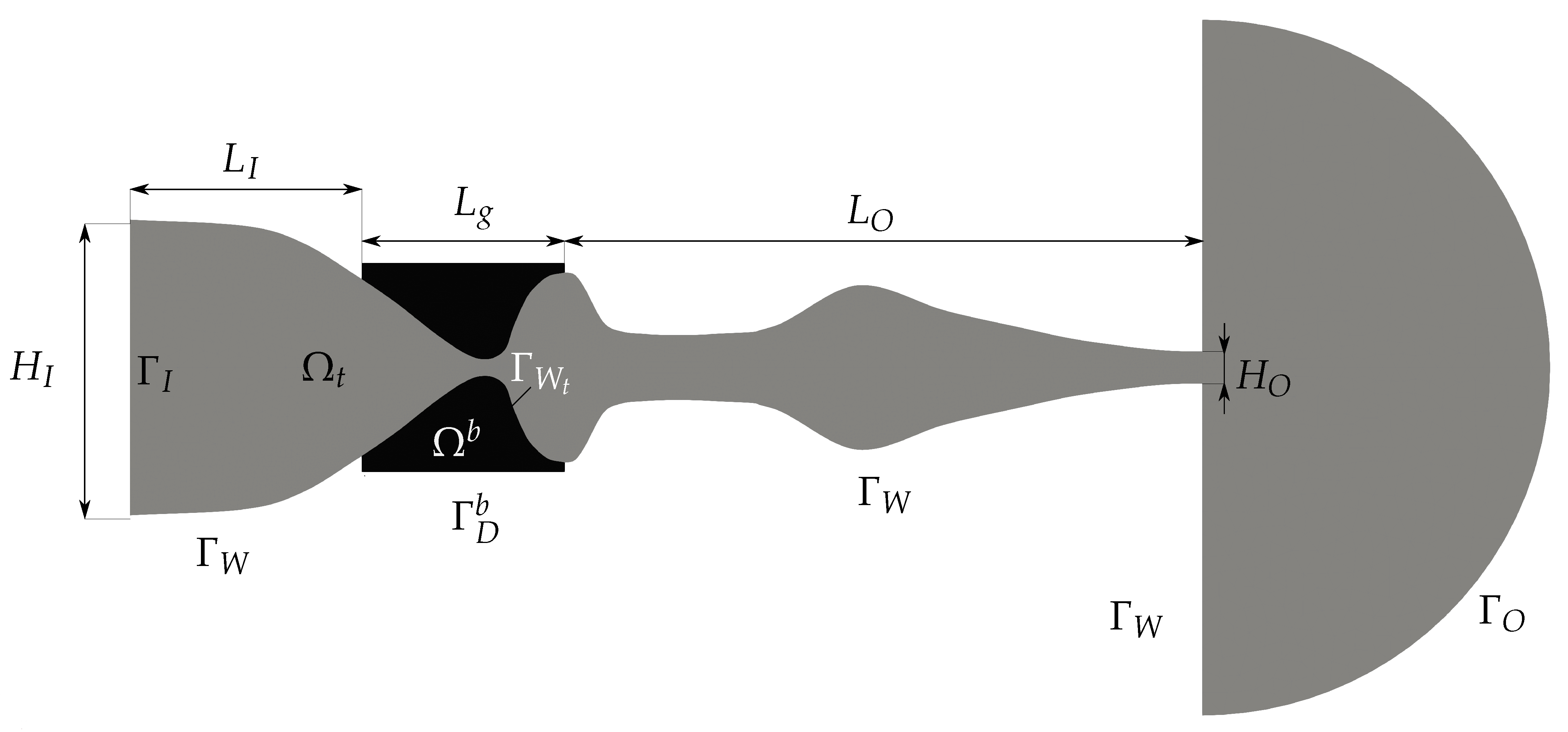
Here, we present numerical results of an FSI problem considering a simplified VFs model excited by airflow. The geometry of the airflow domain , which models the simplified subglottal, supraglottal spaces and a semicircle subdomain with an outlet to a surrounding atmosphere, is given in Figure 2. The boundaries of the airflow domain are considered as the impermeable hard sidewalls of the vocal tract including the vertical segments of the semicircle at the outlet. The computational domain marks the elastic VFs with the surface , which creates an interface with the airflow domain. The VFs are fixed at the boundaries denoted by .
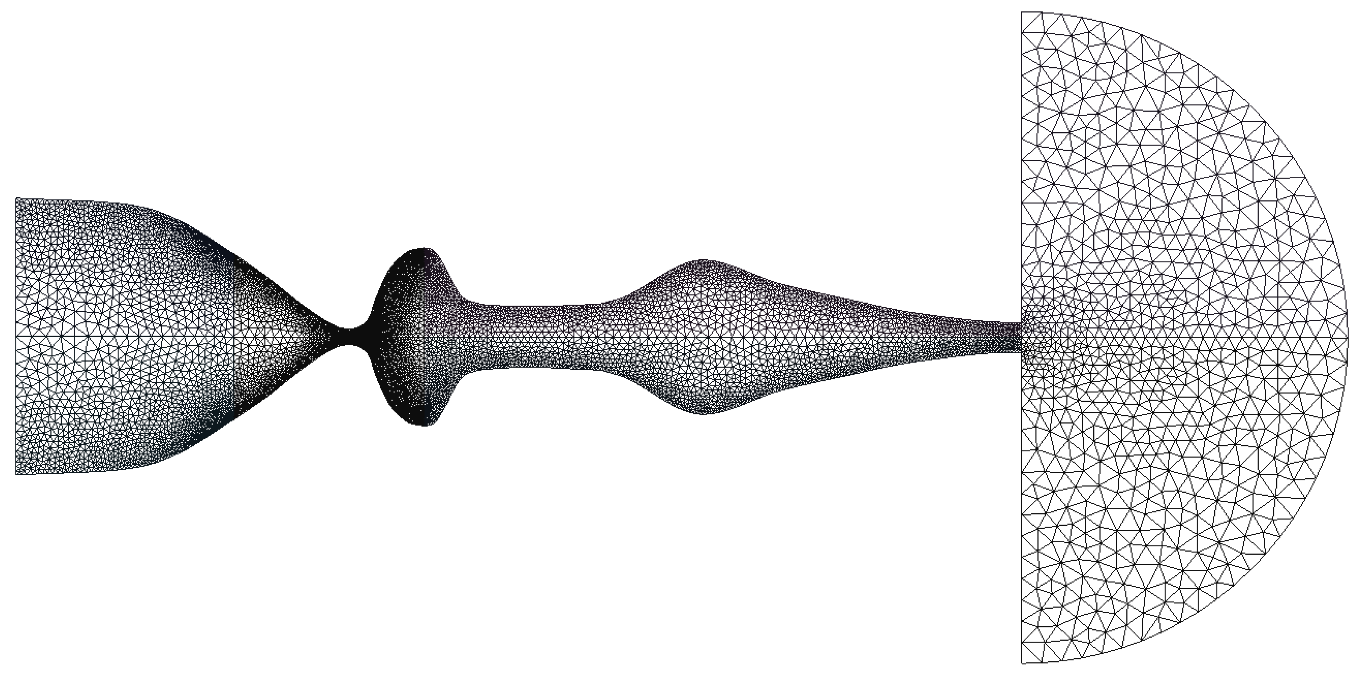
The fluid flow problem is computed on the triangulation with 17,652 elements; see Figure 3.
Further, for the flow problem, the following input data are used:
| inlet velocity | m s, |
| dynamic viscosity | kg m s, |
| inlet density | kg m, |
| initial outlet pressure | Pa, |
| Reynolds number | , |
| heat conduction coeff. | kg m s K, |
| specific heat | m s K, |
| Poisson adiab. const. | . |
For the fluid solver, the STDGM with a polynomial approximation of degree 2 in space and degree 1 in time is used. In the case of the elasticity solver, the IIPG version of the DGM with the penalization constant for inner faces and for boundary edges is employed. The stabilization parameters and from (16) are set to . The time step is set to s. For the first 1000 time steps, the fluid flow is computed with the fixed boundary. Then, the part of the boundary is released and we solve the FSI problem.
The elastic VFs are modeled by isotropic material of the density kg m. The VF model is formed by four subdomains with different elastic properties, as shown in Figure 4 and Table 4. Every VF contains 5118 elements.
The initial displacement and the initial deformation velocity are set to be zero. On the bottom, right and left straight parts of the boundary, we prescribe a homogeneous Dirichlet boundary condition (25) and on the curved part of the boundary, the Neumann boundary condition (26). The damping coefficient is set to s. For the solution of the dynamic elasticity problem, we employ the NIPG version of the DGM, where the penalization constant is set to .
For the solution of the static elasticity problem (48), we employ the NIPG version of the DGM with the penalization constant . Then, the DG solution of the ALE discrete problem (48) is interpolated to a continuous approximation.
The strong coupling algorithm described in Section 4.3 with the prescribed tolerance is used. The prescribed tolerance was usually reached after two to three coupling subiterations.
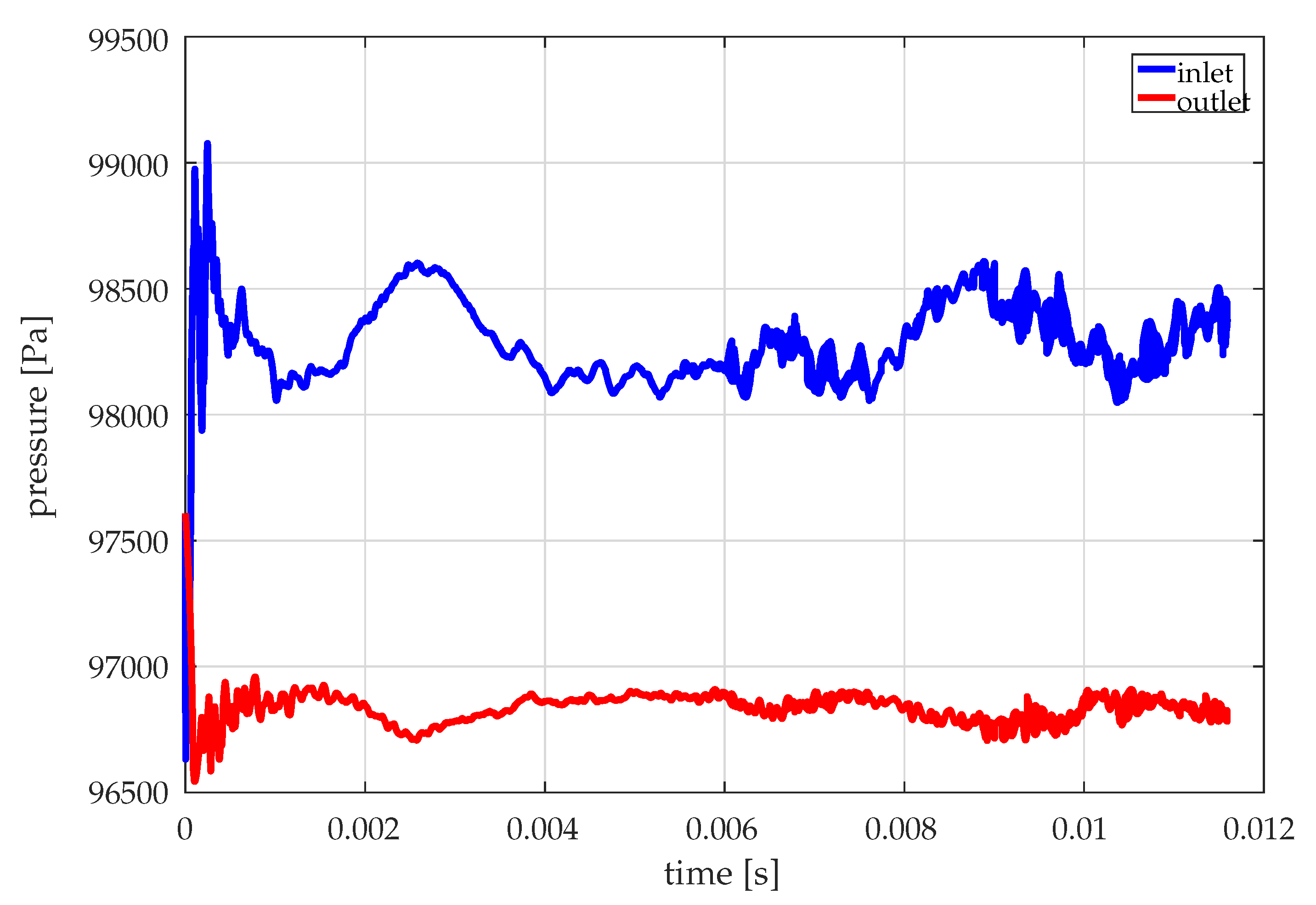
Figure 5 shows the airflow velocity field in the subglottal and supraglottal regions at five time instants of the VFs self-oscillation. In these time instants, different jet declination behind the channel constriction, i.e., the so-called ”Coanda effect”, can be observed, with the maximum flow velocity ca. 80 m/s. It corresponds to the Mach number . Similarly as in Figure 5, we see the distribution of the pressure in Figure 6. The maximum air pressure is approximately constant in the subglottic part of the computational model. The minima of the pressure corresponds to centers of the vortices created in the supraglottal region and traveling to the outlet. Figure 7 shows the fluid pressure fluctuations in the middles of the inlet and outlet. The value vibrations are caused by the non-stationary flow behavior. In Figure 8, we can see the time dependence of the average values across the inlet and outlet. The average mean difference between the inlet and outlet pressure is around 1 kPa, which is in the range of subglottic pressure for ordinary phonation.
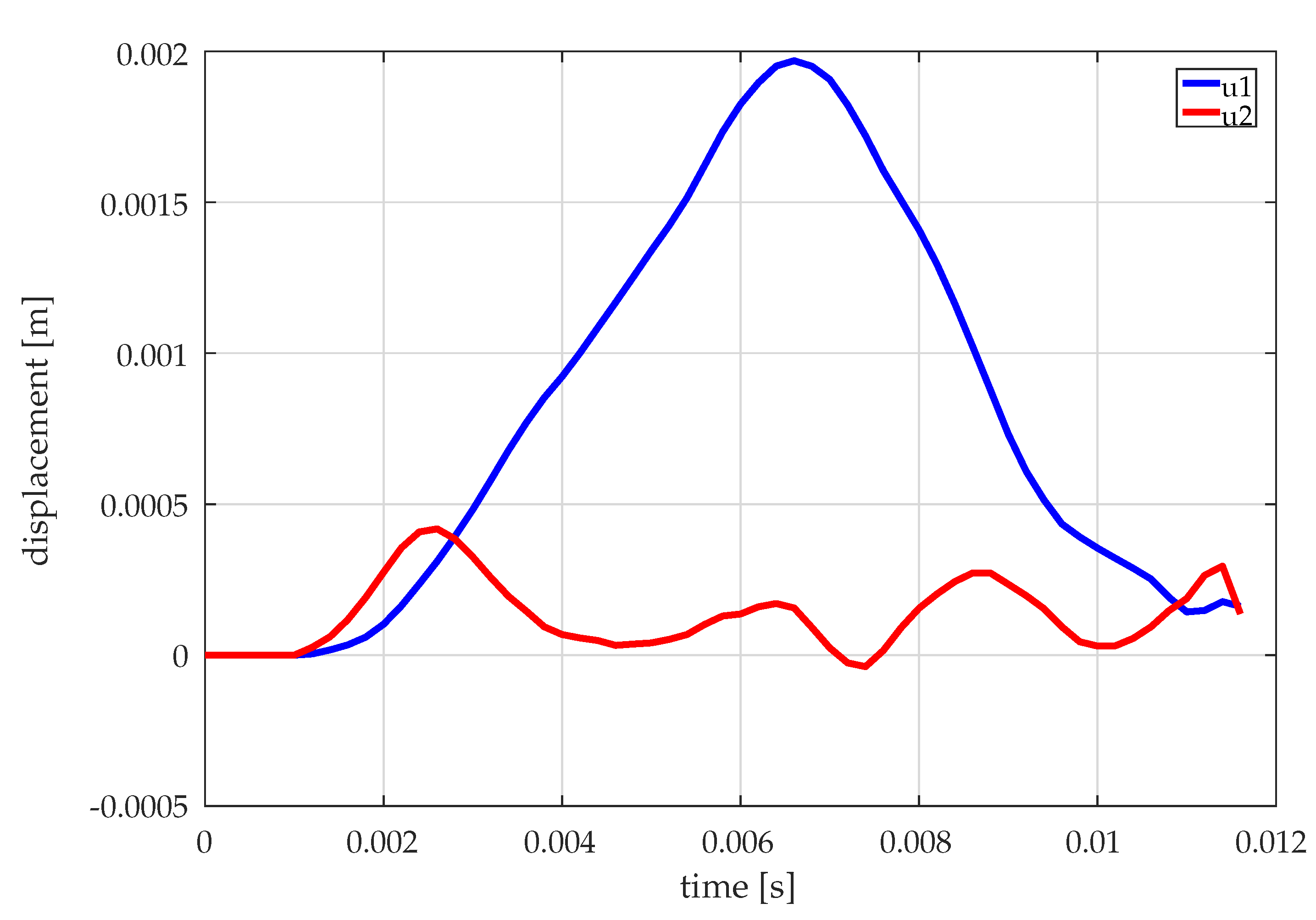
Figure 9 shows the displacement of the top of the vocal fold in horizontal () and vertical () directions. The numerical simulation of the VF vibrations started from zero initial conditions and static fluid forces deformed the VFs statically, predominantly in the horizontal direction. This effect shifted the mean value of VFs self-oscillations downstream. The vibration amplitudes with frequency ca. 100 Hz in the horizontal direction are dominant.
Comparison of the FSI Results for Linear and Two Nonlinear Elasticity Models
This section will be devoted to the analysis of nonlinear elasticity models in comparison with linear ones. We compare the linear strain tensor and the nonlinear strain tensor , defined by (32). For the linear elasticity, the stress tensor depends on the strain tensor , and in the case of nonlinear elasticity, the stress tensor depends on , where .
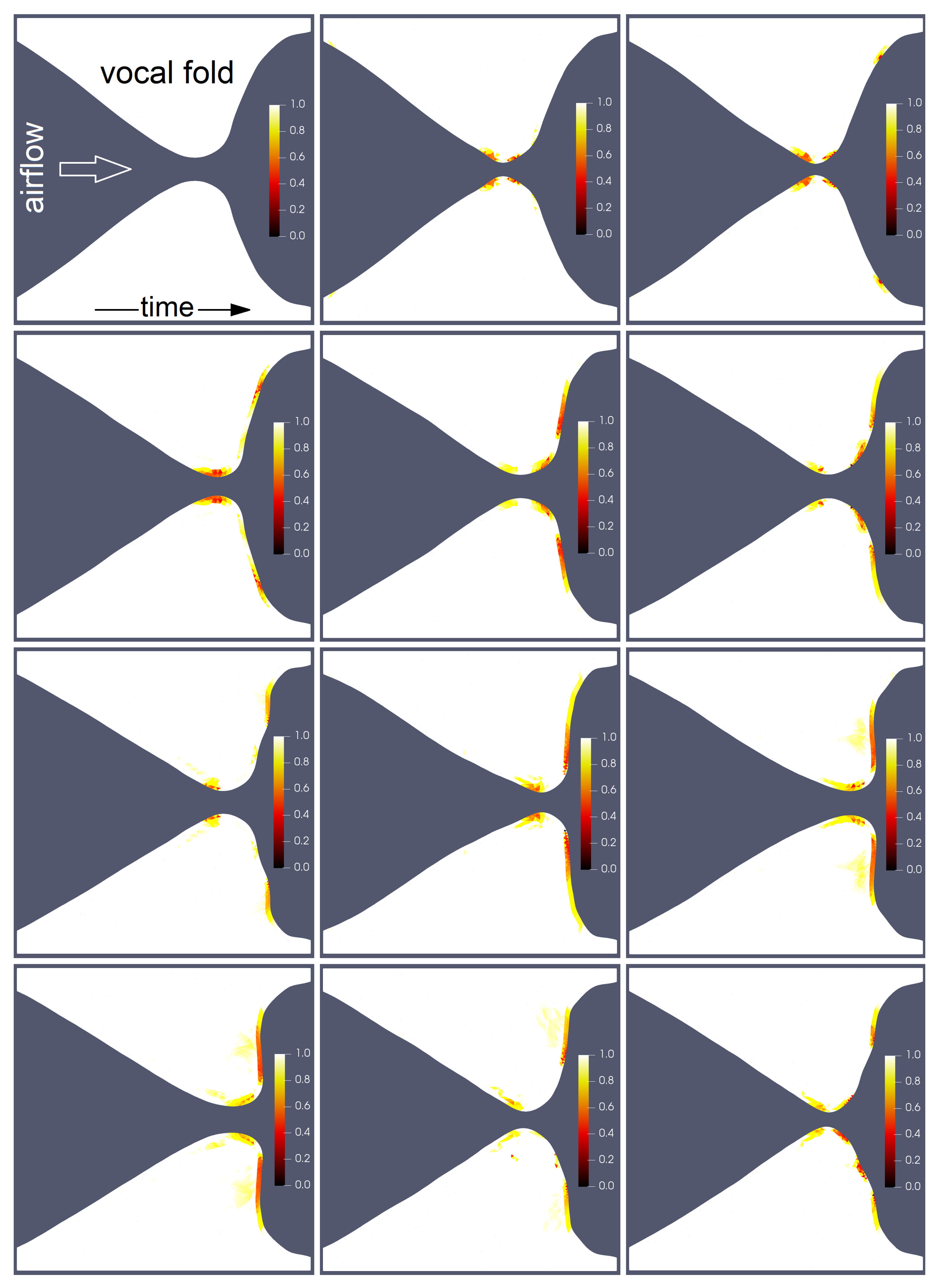
The influence of the nonlinear part of the strain tensor is given by the ratio
If , then the nonlinear part of the strain tensor is very small and the linear elasticity model is sufficient, but if , then it is necessary to use a nonlinear elasticity model.
First, we are concerned with the analysis of the neo-Hookean model. In this case, Figure 10 shows the numerical simulation of the VFs self-oscillations from the beginning of the FSI computation at 12 time instants. Figure 11 shows in detail the deformation of the VFs at two time instants for a maximal and minimal glottal gap. In Figure 10 and Figure 11, the case is depicted by white and the case by a dark red color. The nonlinear part of the strain tensor takes effect near the VFs surface, especially in the narrowest part of the glottal channel and on the superior surface of the VFs. Therefore, to correctly capture deformations of the VFs, it is necessary to use a nonlinear elasticity model.
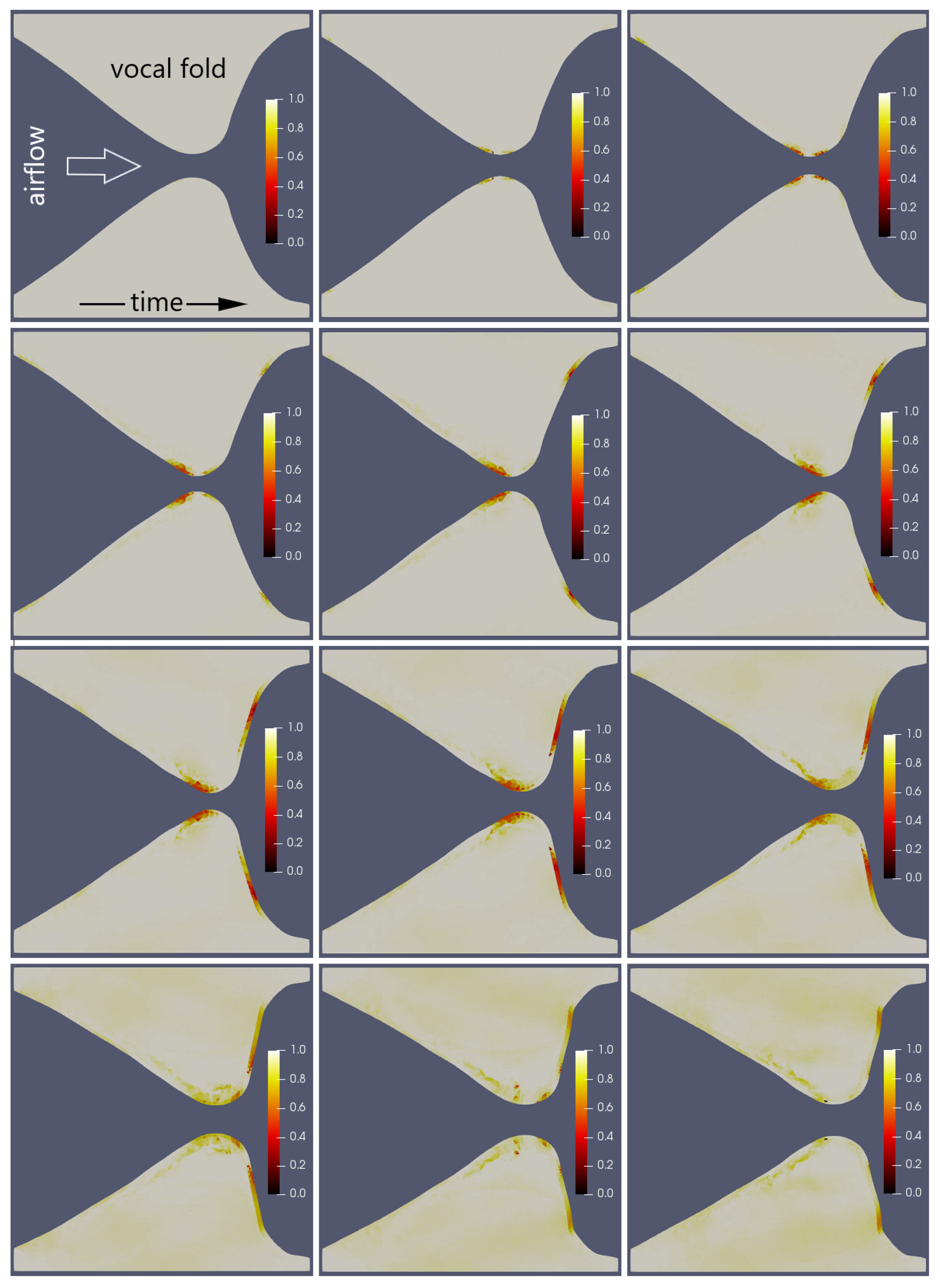
Further, we present the results obtained for the St. Venant–Kirchhoff nonlinear elasticity model. From the comparison of Figure 10 and Figure 12 and details in Figure 11 and Figure 13, we see that the results for deformations of the VFs during self-oscillations are very similar. The St. Venant–Kirchhoff model shows slightly higher influence of the nonlinearity than the neo-Hookean material model of the VFs.
8. Discussion and Conclusions
This paper deals with the application of the space-time discontinuous Galerkin method to the numerical solution of the compressible flow in time-dependent domains, described by the compressible Navier–Stokes system, and to the nonlinear dynamic elasticity problems. This is described by the St. Venant–Kirchhoff and the neo-Hookean models. The main novelty is the numerical simulation of the fluid–structure interaction, namely, the vocal folds vibrations excited by the compressible flow. The elastic vocal folds consist of several layers with different material characteristics.
First, the applicability of the STDGM to the solution of a nonlinear dynamic elasticity is tested on a benchmark problem published in [40], where the elastic deformation of a vibrating beam is considered. Then the coupled fluid–structure problem is numerically solved. An important part of the presented study is oriented to the solution of the question whether the linear or nonlinear elasticity models of the vocal folds are more suitable. It follows from our analysis that the use of nonlinear elasticity models are more adequate than the linear model. The differences between the results obtained by the two nonlinear material models are very small.
In future studies, the identification of the generated acoustic signal and a remeshing in the case of the full glottal channel closure during the vocal folds oscillation period should be analyzed.
Author Contributions
Conceptualization, M.B., M.F., J.H. and A.K.; formal analysis, M.B., M.F., J.H. and A.K.; investigation, M.B., M.F., J.H. and A.K.; software, M.B. and A.K.; visualization, M.B. and A.K.; writing—original draft, M.B., M.F., J.H. and A.K.; writing—review and editing, M.B., M.F., J.H. and A.K. All authors have read and agreed to the published version of the manuscript.
Funding
The research was supported by the grant 20-01074S (M. Feistauer) and the grant 19-04477S (J. Horáček) of the Czech Science Foundation, and the research of M. Balázsová was supported by the Ministry of Education, Youth and Sports of the Czech Republic under the OP RDE grant number CZ.02.1.01/0.0/0.0/16 019/0000778/Centre for Advanced Applied Sciences, group THEORY.
Institutional Review Board Statement
Not applicable.
Informed Consent Statement
Not applicable.
Data Availability Statement
The data presented in this study are available on request from the corresponding author. The data are not publicly available due to the sheer large size of the dataset.
Acknowledgments
The research was supported by the grant 20-01074S (M. Feistauer) and the grant 19-04477S (J. Horáček) of the Czech Science Foundation and the research of M. Balázsová was supported by the Ministry of Education, Youth and Sports of the Czech Republic under the OP RDE grant number CZ.02.1.01/0.0/0.0/16 019/0000778/Centre for Advanced Applied Sciences, group THEORY.
Conflicts of Interest
The authors declare no conflict of interest. The funders had no role in the design of the study; in the collection, analyses, or interpretation of data; in the writing of the manuscript, or in the decision to publish the results.
Abbreviations
The following abbreviations are used in this manuscript:
| ALE | arbitrary Lagrangian–Eulerian (method) |
| DGM | discontinuous Galerkin method |
| FE | finite element |
| FSI | fluid–structure interaction |
| N-S | Navier–Stokes |
| STDGM | space-time discontinuous Galerkin method |
| VFs | vocal folds |
References
- Fung, Y.C. An Introduction to the Theory of Aeroelaticity; Dover Publications: New York, NY, USA, 1969. [Google Scholar]
- Dowell, E.H. Aeroelasticity of Plates and Shells; Kluwer: Dordrecht, The Netherlands, 1974. [Google Scholar]
- Naudasher, E.; Rockwell, D. Flow-Induced Vibrations; A. A. Balkema: Rotterdam, The Netherlands, 1994. [Google Scholar]
- Dowell, E.H. A modern Course in Aeroelaticity; Kluwer: Dordrecht, The Netherlands, 1995. [Google Scholar]
- Bisplinghoff, R.L.; Ashley, H.; Halfman, R.L. Aeroelaticity; Dover: New York, NY, USA, 1996. [Google Scholar]
- Paidoussis, M.P. Fluid-Structure Interactions. Slender Structures and Axial Flow, Vol I.; Academic Press: San Diego, CA, USA, 1998. [Google Scholar]
- Paidoussis, M.P. Fluid-Structure Interactions. Slender Structures and Axial Flow, Vol II.; Academic Press: London, UK, 2004. [Google Scholar]
- Mittal, R.; Erath, B.D.; Plesniak, M.W. Fluid dynamics of human phonation and speech. Annu. Rev. Fluid Mech. 2013, 45, 437–467. [Google Scholar] [CrossRef]
- Seo, J.H.; Mittal, R. A higher-order immersed boundary method for acoustic wave scattering and low-Mach number flow-induced sound in complex geometries. J. Comput. Phys. 2011, 230, 1000–1019. [Google Scholar] [CrossRef] [Green Version]
- Zheng, X.; Bielamowicz, S.; Luo, H.; Mittal, R. A computational study of the effect of false vocal folds on glottal flow and vocal fold vibration during phonation. Ann. Biomed. Eng. 2009, 37, 625–642. [Google Scholar] [CrossRef] [Green Version]
- Dolejší, V.; Feistauer, M. Discontinuous Galerkin Method—Analysis and Applications to Compressible Flow; Springer: Cham, Switzerland, 2015. [Google Scholar]
- Pořízková, P.; Kozel, K.; Horáček, J. Flows in convergent channel: Comparison of numerical results of different mathematical models. Computing 2013, 95, 573–585. [Google Scholar] [CrossRef]
- Šidlof, P.; Zorner, S.; Huppe, A. A hybrid approach to the computational aeroacoustics of human voice production. Biomech. Model. Mechanobiol. 2014, 14, 473–488. [Google Scholar] [CrossRef] [PubMed]
- Ishizaka, K.; Flanagan, J.L. Synthesis of voiced sounds from a two-mass model of the vocal cords. Bell Syst. Tech. 1972, 51, 1233–1268. [Google Scholar] [CrossRef]
- Liljencrants, J. A translating and rotating mass model of the vocal folds. Speech Transm. Lab. Q. Prog. Status Rep. 1991, 1, 1–18. [Google Scholar]
- Titze, I.R. Phonation threshold pressure: A missing link in glottal aerodynamics. J. Acoust. Soc. Am. 1992, 91, 2928–2934. [Google Scholar] [CrossRef]
- Story, B.H.; Titze, I.R. Voice simulation with a body cover model of the vocal folds. J. Acoust. Soc. Am. 1995, 97, 1249–1260. [Google Scholar] [CrossRef]
- Sváček, P.; Horáček, J. Finite element approximation of flow induced vibrations of human vocal folds model: Effects of inflow boundary conditions and the length of subglottal and supraglottal channel on phonation onset. Appl. Math. Comput. 2018, 319, 178–194. [Google Scholar] [CrossRef]
- Feistauer, M.; Kučera, V.; Prokopová, J. Discontinuous Galerkin solution of compressible flow in time-dependent domains. Math. Comput. Simul. 2010, 80, 1612–1623. [Google Scholar] [CrossRef]
- Hasnedlová, J.; Feistauer, M.; Horáček, J.; Kosík, A.; Kučera, V. Numerical simulation of fluid-structure interaction of compressible flow and elastic structure. Computing 2013, 95, 343–361. [Google Scholar] [CrossRef]
- Feistauer, M.; Horáček, J.; Sváček, P. Numerical Simulation of Fluid-Structure Interaction Problems with Applications to Flow in Vocal Folds. In Fluid-Structure Interaction and Biomedical Applications; Bodnár, T., Galdi, G.P., Nečasová, Š., Eds.; Springer: Basel, Switzerland, 2014. [Google Scholar]
- Hatrmann, R.; Houston, P. Symmetric interionr penalty DG methods for the compressible Navier-Stokes equations I: Method formulation. Int. J. Numer. Anal. Model. 2006, 1, 1–20. [Google Scholar]
- Dumbser, M. Arbitrary high order PNPM schemes on unstructured meshes for the compressible Navier-Stokes equations. Comput. Fluids 2010, 39, 60–76. [Google Scholar] [CrossRef]
- Dolejší, V. On the discontinuous Galerkin method for the numerical solution of the Navier—Stokes equations. Int. J. Numer. Methods Fluids 2004, 45, 1083–1106. [Google Scholar] [CrossRef]
- Dolejší, V. Semi-implicit interior penalty discontinuous Galerkin methods for viscous compressible flows. Commun. Comput. Phys. 2008, 4, 231–274. [Google Scholar]
- Česenek, J.; Feistauer, M.; Kosík, A. DGFEM for the analysis of airfoil vibrations induced by compressible flow. ZAMM Z. Angew. Math. Mech. 2013, 93, 387–402. [Google Scholar] [CrossRef]
- Feistauer, M.; Hasnedlová-Prokopová, J.; Horáček, J.; Kosík, A.; Kučera, V. DGFEM for dynamical systems describing interaction of compressible fluid and structures. J. Comput. Appl. Math. 2013, 254, 17–30. [Google Scholar] [CrossRef]
- Kosík, A. Fluid-Structure Interaction. Ph.D. Thesis, Department of Numerical Mathematics, Faculty of Mathematics and Physics, Charles University in Prague, Prague, Czech Republic, 2016. [Google Scholar]
- Ciarlet, P.G. The Finite Element Method for Elliptic Problems; North-Holland: Amsterdam, The Netherlands, 1979. [Google Scholar]
- Feistauer, M.; Felcman, J.; Straškraba, I. Mathematical and Computational Methods for Compressible Flow; Clarendon Press: Oxford, UK, 2003. [Google Scholar]
- Feistauer, M.; Kučera, V. On a robust discontinuous Galerkin technique for the solution of compressible flow. J. Comput. Phys. 2007, 224, 208–221. [Google Scholar] [CrossRef]
- Ciarlet, P.G. Mathematical Elasticity, Volume I, Three-Dimensional Elasticity; Volume 20 of Studies in Mathematics and Its Applications; Elsevier Science Publishers B.V.: Amsterdam, The Netherlands, 1988. [Google Scholar]
- Deuflhard, P. Newton Methods for Nonlinear Problems, Affine Invariance and Adaptive Algorithms; Springer Series in Computational Mathematics 35; Springer: Berlin/Heidelberg, Germany, 2004. [Google Scholar]
- Davis, T.A.; Duff, I.S. A combined unifrontal/multifrontal method for unsymmetric sparse matrices. ACM Trans. Math. Softw. 1999, 25, 1–19. [Google Scholar] [CrossRef]
- Saad, Y.; Schultz, M.H. GMRES: A generalized minimal residual algorithm for solving nonsymmetric linear systems. SIAM J. Sci. Statist. Comput. 1986, 7, 856–869. [Google Scholar] [CrossRef] [Green Version]
- Young, Z.; Mavriplis, D.J. Unstructured dynamic meshes with higher-order time integration schemes for the unsteady Navier-Stokes equations. In Proceedings of the 43rd AIAA Aerospace Sciences Meeting and Exhibit, AIAA Paper 1222, Reno, NV, USA, 10–13 January 2005. [Google Scholar]
- Badia, S.; Codina, R. On some fluid-structure iterative algorithms using pressure segregation methods. Application to aeroelesticity. Int. J. Numer. Methods Eng. 2007, 72, 46–71. [Google Scholar] [CrossRef]
- Fernandez, M.A.; Moubachir, M. A Newton method using exact jacobians for solving fluid-structure coupling. Comput. Struct. 2005, 83, 127–142. [Google Scholar] [CrossRef] [Green Version]
- Richter, T. Goal oriented error estimation for fluid-structure interaction problems. Comput. Methods Appl. Mech. Eng. 2012, 223–224, 28–42. [Google Scholar] [CrossRef] [Green Version]
- Turek, S.; Hron, J. Proposal for numerical benchmarking of fluid-structure interaction between an elastic object and laminar incompressible flow. In Fluid-Structure Interaction: Modelling, Simulation, Optimisation; Bungartz, H.J., Schäfer, M., Eds.; Springer: Berlin/Heidelberg, Germany, 2006; pp. 37–385. [Google Scholar]
Figure 1.
Setup of the benchmark problem: elastic beam attached to a rigid cylinder.

Figure 2.
Computational domain at time : mm, mm, mm, mm, mm. The radius of the semicircle subdomain is cm.
Figure 2.
Computational domain at time : mm, mm, mm, mm, mm. The radius of the semicircle subdomain is cm.

Figure 3.
Triangulation of the fluid domain.

Figure 4.
Nonhomogeneous model of VFs formed by four layers with triangulation. Modeled layers: 1. muscle, 2. ligament, 3. superficial lamina propria and 4. epithelium.
Figure 4.
Nonhomogeneous model of VFs formed by four layers with triangulation. Modeled layers: 1. muscle, 2. ligament, 3. superficial lamina propria and 4. epithelium.

Figure 5.
Velocity field in the glottal region at five time instants () of the vocal folds self-oscillation.
Figure 5.
Velocity field in the glottal region at five time instants () of the vocal folds self-oscillation.

Figure 6.
Distribution of the pressure in the glottal region at five time instants () of the vocal folds self-oscillation.
Figure 6.
Distribution of the pressure in the glottal region at five time instants () of the vocal folds self-oscillation.

Figure 7.
The fluid pressure fluctuation at the middle point of inlet and at the middle point of the outlet of the vocal tract.
Figure 7.
The fluid pressure fluctuation at the middle point of inlet and at the middle point of the outlet of the vocal tract.

Figure 8.
Average fluid pressure on the inlet and on the outlet .

Figure 9.
Displacement of the top of the vocal fold.

Figure 10.
Visualization of the VFs vibrations and the ratios R of the norms of linear and nonlinear strain tensors at twelve time instants. Computed by the neo-Hookean model.
Figure 10.
Visualization of the VFs vibrations and the ratios R of the norms of linear and nonlinear strain tensors at twelve time instants. Computed by the neo-Hookean model.

Figure 11.
Details of VFs deformations and the ratios R of the norms of linear and nonlinear strain tensors for the smallest and the largest glottal gap. Computed by the neo-Hookean elasticity model.
Figure 11.
Details of VFs deformations and the ratios R of the norms of linear and nonlinear strain tensors for the smallest and the largest glottal gap. Computed by the neo-Hookean elasticity model.

Figure 12.
Visualization of the VFs vibrations and the ratios R of the norms of linear and nonlinear strain tensors at twelve time instants. Computed by the St. Venant–Kirchhoff elasticity model.
Figure 12.
Visualization of the VFs vibrations and the ratios R of the norms of linear and nonlinear strain tensors at twelve time instants. Computed by the St. Venant–Kirchhoff elasticity model.

Figure 13.
Details of VFs deformations and the ratios R of the norms of linear and nonlinear strain tensors for the smallest and the largest glottal gap. Computed by the St. Venant–Kirchhoff elasticity model.
Figure 13.
Details of VFs deformations and the ratios R of the norms of linear and nonlinear strain tensors for the smallest and the largest glottal gap. Computed by the St. Venant–Kirchhoff elasticity model.


Table 1.
Comparison of the position of point A for the reference and STDGM results with decreasing time step , for the St. Venant–Kirchhoff model. The displacements and are written in the format “mean value ± amplitude” and frequency. The row marked by ”ref” shows the reference benchmark values published in [40].
| Method | f [Hz] | f [Hz] | |||
|---|---|---|---|---|---|
| ref | |||||
| STDGM | 0.04 | ||||
| STDGM | 0.02 | ||||
| STDGM | 0.01 | ||||
| STDGM | 0.005 |
Table 2.
Comparison of the position of point A for the STDGM with decreasing time step for the neo-Hookean model.
Table 2.
Comparison of the position of point A for the STDGM with decreasing time step for the neo-Hookean model.
| Method | f [Hz] | f [Hz] | |||
|---|---|---|---|---|---|
| STDGM | 0.04 | ||||
| STDGM | 0.02 | ||||
| STDGM | 0.01 | ||||
| STDGM | 0.005 |
Table 3.
Comparison of the position of point A for STDGM with for St. Venant–Kirchhoff material and different meshes defined by number of elements.
Table 3.
Comparison of the position of point A for STDGM with for St. Venant–Kirchhoff material and different meshes defined by number of elements.
| Num. of Elem. | f [Hz] | f [Hz] | |||
|---|---|---|---|---|---|
| ref | |||||
| 722 | 0.02 | ||||
| 1348 | 0.02 | ||||
| 2822 | 0.02 |
Table 4.
Prescribed material constants for the VFs model: Young modulus, Poisson ratio and Lamé parameters for different layers, ordered from the lower layer to the upper layer. See Figure 4 for the visualization of the corresponding subdomains.
Table 4.
Prescribed material constants for the VFs model: Young modulus, Poisson ratio and Lamé parameters for different layers, ordered from the lower layer to the upper layer. See Figure 4 for the visualization of the corresponding subdomains.
| Layer | ||||
|---|---|---|---|---|
| 1. layer (orange) | 17,143 | 4285 | ||
| 2. layer (yellow) | 11,430 | 2857 | ||
| 3. layer (blue) | 33,110 | 335 | ||
| 4. layer (red) | 142,857 | 35,714 |
Publisher’s Note: MDPI stays neutral with regard to jurisdictional claims in published maps and institutional affiliations. |
© 2021 by the authors. Licensee MDPI, Basel, Switzerland. This article is an open access article distributed under the terms and conditions of the Creative Commons Attribution (CC BY) license (https://creativecommons.org/licenses/by/4.0/).
Share and Cite
MDPI and ACS Style
Balázsová, M.; Feistauer, M.; Horáček, J.; Kosík, A. Vibrations of Nonlinear Elastic Structure Excited by Compressible Flow. Appl. Sci. 2021, 11, 4748. https://doi.org/10.3390/app11114748
AMA Style
Balázsová M, Feistauer M, Horáček J, Kosík A. Vibrations of Nonlinear Elastic Structure Excited by Compressible Flow. Applied Sciences. 2021; 11(11):4748. https://doi.org/10.3390/app11114748
Chicago/Turabian StyleBalázsová, Monika, Miloslav Feistauer, Jaromír Horáček, and Adam Kosík. 2021. "Vibrations of Nonlinear Elastic Structure Excited by Compressible Flow" Applied Sciences 11, no. 11: 4748. https://doi.org/10.3390/app11114748
Note that from the first issue of 2016, this journal uses article numbers instead of page numbers. See further details here.