
Control of a Round Jet Intermittency and Transition to Turbulence by Means of an Annular Synthetic Jet


Institute of Thermomechanics of the Czech Academy of Sciences, Dolejškova 5, 182 00 Prague, Czech Republic
*
Author to whom correspondence should be addressed.
Actuators 2021, 10(8), 185; https://doi.org/10.3390/act10080185
Submission received: 28 June 2021
/
Revised: 27 July 2021
/
Accepted: 29 July 2021
/
Published: 5 August 2021
(This article belongs to the Special Issue Flow Control by Means of Synthetic Jet Actuators)
Abstract
:This paper deals with active control of a continuous jet issuing from a long pipe nozzle by means of a concentrically placed annular synthetic jet. The experiments in air cover regimes of laminar, transitional, and turbulent main jet flows (Reynolds number ranges 1082–5181). The velocity profiles (time-mean and fluctuation components) of unforced and forced jets were measured using hot-wire anemometry. Six flow regimes are distinguished, and their parameter map is proposed. The possibility of turbulence reduction by forcing in transitional jets is demonstrated, and the maximal effect is revealed at Re = 2555, where the ratio of the turbulence intensities of the forced and unforced jets is decreased up to 0.45.
1. Introduction
Fluid jet flows are one of the free shear flows that occur without a direct impact of wall boundaries on fluid motion. The fluid motion can be laminar or turbulent in character. The governing parameter is the Reynolds number, Re = Um D/ν, where Um is the mean velocity through the nozzle producing the jet, D is the characteristic scale, which is the nozzle diameter for round jets, and ν is the kinematic viscosity of the working fluid.
The jet flows were investigated in many theoretical, experimental, and applied studies; see Schlichting [1], Abramovich [2], and Blevins [3]. For a given geometry, the laminar-turbulent transition (or onset of turbulence) is linked with the critical Reynolds number, Rec. While the flows through pipes and ducts can be laminar up to a relatively high Re (typically Rec~2300), the transition in jets occurs at Re and is about two orders of magnitude smaller due to an absence of the wall stabilization effects. For example, Bejan [4] specified Rec~10–30 for round jet flows.
The laminar–turbulent transition is linked with the jet intermittency and occurrence of the coherent structures, as was studied by many authors, e.g., Crow and Champagne [5], Yule [6], Hussain and Husain [7], Zaman [8], Komori and Ueda [9], Thomas [10], and Matsuda and Sakakibara [11].
The vortex structures originate from instabilities in boundary layers in the nozzle. They are shed from the nozzle and drifted by the shear layer. The initial structures are developed into large-scale coherent structures. The possibility to control these processes remains a great challenge for researchers, see Hussain and Husain [7], Fiedler and Fernholz [12], and Gad-el-Hak [13]. Active control was investigated using periodic forcing at one or more frequencies. The physical mechanism of such control lies in the modification of the coherent structures; therefore, the appropriate forcing frequencies can be derived according to the behavior of unexcited jets. The characteristic passage frequencies of the structures in a jet decrease along the jet mixing layer, while their space scale proportionately grows. The dimensionless frequency can be quantified as the Strouhal number St = f D/Um, where f is the frequency. The characteristic frequencies of round jets were experimentally investigated by Crow and Champagne [5] by introducing small artificial external excitations. They considered that the highest sensitivity indicates the most amplified mode, known as the most preferred mode. This mode was revealed at the Strouhal number St = 0.3–0.35 [5].
Liu and Sullivan [14] measured the natural frequency of an unexcited round jet relating to the jet–column mode, concluding that the Strouhal number decreases from 1.23 near the exit to 0.61. Moreover, a stepwise evolution of the vortex passage frequency with a distinct hysteretic effect was presented [14]. Note that similar stepwise and hysteretic effects were found for high-frequency acoustic forcing at St = 3.54 by Kibens [15].
Thomas [10] concluded a bit wider range of St from 0.25 to 0.85 due to a variation in the boundary layer thickness at the nozzle exit. Consistently, Vlasov and Ginevski [16] found that the Strouhal number value decreases from about St = 5–1 near the nozzle to St = 0.3–0.5 at the end of the initial region.
Lepičovský et al. [17] investigated high-speed round jets under strong upstream acoustic excitations (up to 141 dB) at Strouhal numbers of 0.4, 0.5, and 0.6. They found that the upstream acoustic excitation can enhance flow turbulence, jet spreading rate, and fluid mixing. The effects were significant at the end of the jet potential core due to a promoted generation of the large-scale structures. Similar results were found by Vlasov and Ginevski [16], who revealed that low-frequency acoustic excitations at Strouhal numbers in the range of 0.2–0.6 enhance flow turbulence, jet spreading rate, and fluid mixing through the promotion of large vortices. On the other hand, high frequency forcing at St = 2–5 reduced flow turbulence, jet spreading rate, and fluid mixing through the promotion of small vortices.
An acoustic forcing at two frequencies was investigated by Cho et al. [18]. They revealed that the vortex pairing can be controlled, and the mixing rate can be enhanced by the simultaneous forcing at the fundamental and subharmonic frequencies at St = 0.3–0.6. Note that the 0.3 value agrees well with the most preferred mode, as was referred to in the text above [5]. Moreover, a nonpairing advection of vortices was found for higher-frequency excitations at St~0.6–0.9 [18].
Another experimental investigation of the double-frequency excitation was described by Vejražka et al. [19] at St = 0.3–3. They revealed that a very high sensitivity of vortex roll-up processes to a low-frequency excitation, leading to the formation of larger vortices and an enhancement of velocity fluctuations. On the other hand, a higher-frequency excitation supported the roll-up of small vortices with an attenuation of the velocity fluctuations. Moreover, the double-frequency excitation with subharmonic components promoted the vortex merging process [19].
Hwang et al. [20] investigated actively controlled round jets. They used a coaxial arrangement of a central smoothly contoured nozzle with an annular control nozzle. The acoustic excitations were tested at St = 1.2–4.0. The vortex pairing was promoted at St = 1.2, and the heat transfer on the impingement wall was reduced. On the other hand, the excitation at St = 2.4 and 3.0 caused an extension of the potential jet core. Effects of a steady control co-flow or counter-flow were investigated as well [20].
Diep and Sigurdson [21] used a coaxial arrangement with the main round jet and an annular control jet to model a smokestack with an actively controlled plume. A similar arrangement with an annular control jet was investigated by Koso and Kinoshita [22], and two different control mechanisms were distinguished. The first mechanism is induced by actuation by a very weak-magnitude oscillation where the jet spreading rate and the fluid mixing are enhanced, and thus, the velocity is reduced. The second mechanism is produced by a strong actuation, where the momentum of the main and control jets accumulates, and thus, the velocity is increased. In fact, both control jets [21,22] are synthetic jets in character.
The synthetic jet (SJ) is a fluid flow that is “synthesized” from a periodic motion of fluid oscillating between an actuator cavity and its surroundings through an orifice or nozzle [23,24,25,26]. The flow in the actuator nozzle reverses its orientation after each driven cycle and another commonly used expression is the zero-net-mass-flux jet [27,28]. Probably the first working SJ actuator was the pioneering air-jet generator designed and employed by Dauphinee [29]. Since the end of the last century [23], the phenomenon has been investigated in terms of problems of modeling and performance [30,31,32,33,34,35], as well as design and optimization [36,37,38,39,40]. A primary reason for such interest is the potential of SJ for various applications, such as active flow control [27,41,42,43,44,45,46,47,48], convective heat transfer [49,50,51,52,53,54,55,56,57,58,59,60], mixing enhancement, and thrusters for underwater vehicles [26]. Note that the convective heat transfer applications in impinging jet arrangement [49,50,51,52,53,54,55,56,57,58,59,60] are considered as a potentially very promising area for the investigated subject. However, the jet impingement effects are beyond the main scope of this study.
The leitmotif for the present study is a generally accepted idea that external flow oscillation and synthetic jet actuation can be used as an effective flow control tool. The objective of the present study is to experimentally demonstrate and quantify flow control possibilities in the case of a coaxial arrangement of the main and control jets. The main round jet issues from a relatively long straight pipe, and the control jet is an annular synthetic jet. Although such an arrangement has been studied previously in two available journal papers (Diep and Sigurdson [21], Koso and Kinoshita [22]), both papers focused mainly on flow visualization and flow fields. The impact of the flow control (in this particular arrangement) on the transition to turbulence and the intermittency factor has not been studied thus far. Moreover, the present study also revealed the possibility of how to reduce the intensity of turbulence using this particular arrangement.
Problem Parameters
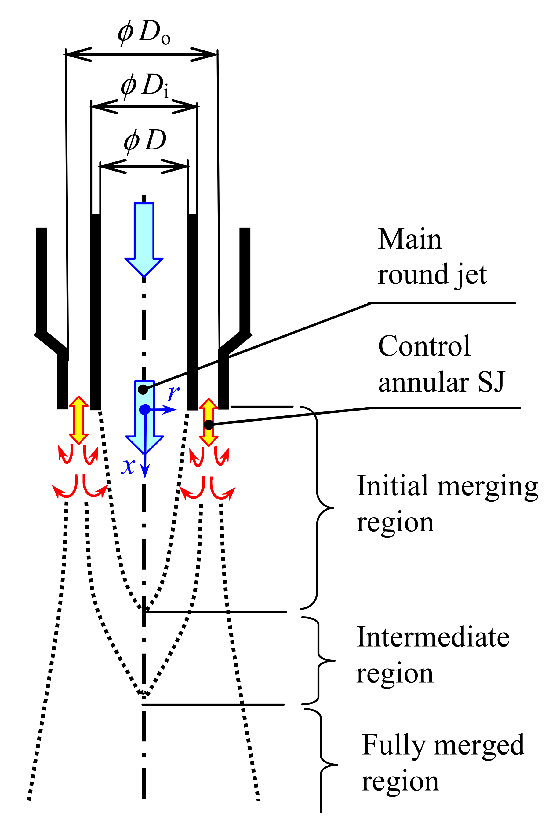
Figure 1 shows a schematic view of the coaxial geometry in which the main round jet is continuous in character and a control jet is the annular SJ. As the main jet issues from a relatively long straight circular pipe (pipe nozzle in short), the pipe flow can be considered approximately developed at the end of the pipe.
The investigated range of Reynolds numbers is Re = Um D/ν = 1082–5181. Due to the chosen Re range, the flow issuing from the pipe end covers laminar, transitional, and turbulent regimes with an intermittent character.
The control SJ issues from an annular nozzle towards the shear layer of the main jet. The characteristic length scale of the SJ is the “stroke length” L0 = U0T, where T is the period (T = 1/f, where f is the driven frequency), and U0 is the characteristic velocity. Assuming the slug flow model (uniform velocity profile at the nozzle exit), U0 can be evaluated as the extrusion orifice velocity averaged over the entire cycle [23].
where TE is the extrusion time (TE = T/2 at a common sinusoidal waveform of u0(t)), and u0 is the velocity at the nozzle exit, x = 0.
The SJ Reynolds number is then defined as ReSJ = U0Do/ν.
The strength of the control SJ relatively to the main jet can be quantified in terms of the ratio of velocities as
where Um is the exit mean velocity of the continuous jet.
2. Experimental Setup and Methods
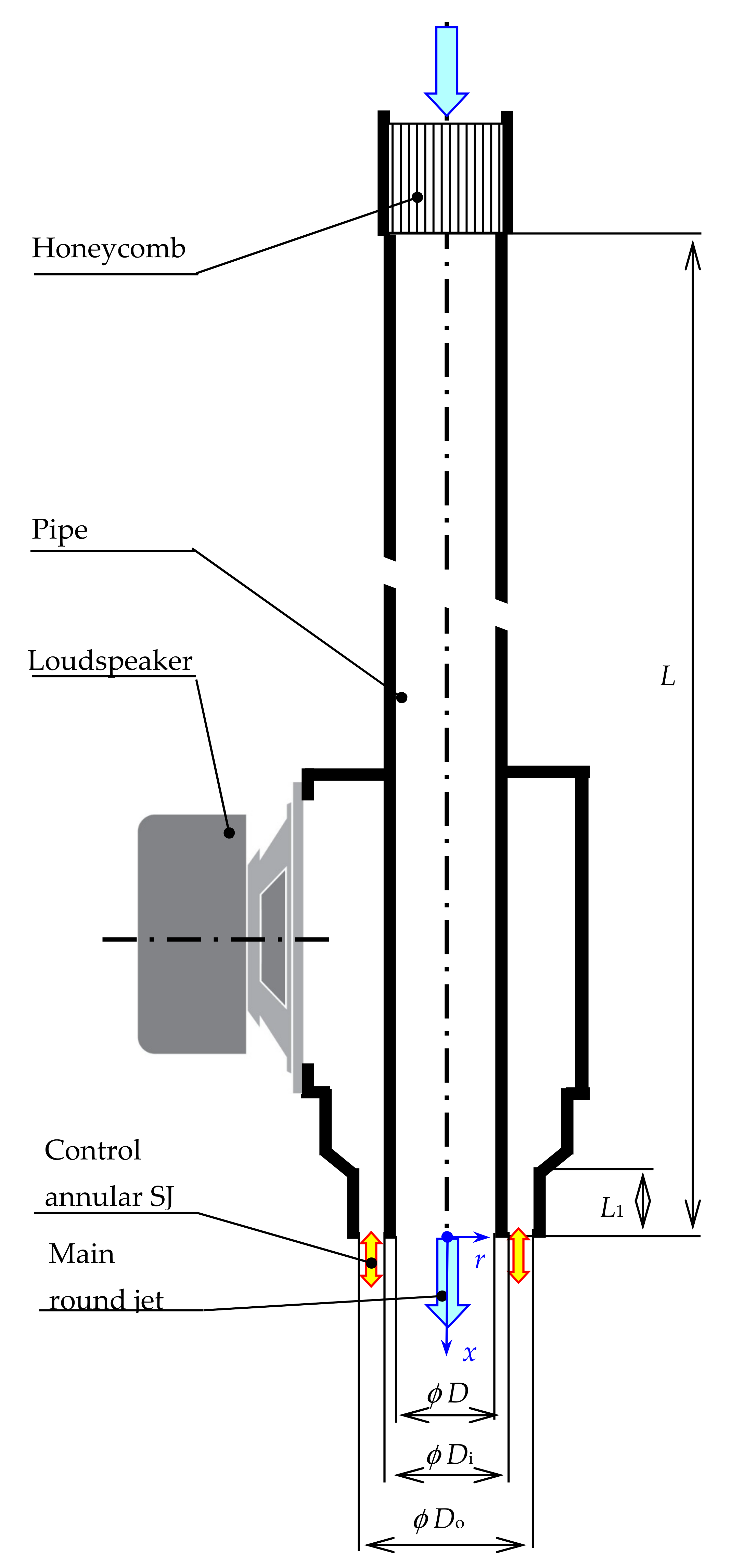
Figure 2 shows a schematic view of the investigated coaxial geometry, including the coordinate system x, r. Following Figure 1, the main round jet is continuous in character and the control jet is the annular SJ. The main jet issues from a relatively long pipe with inner diameter D = 10.05 mm and length of 75 D. The nozzle is oriented vertically, and the flow direction is from top to bottom. Experiments were conducted with air as the working fluid. The air into the pipe was supplied by a compressor, and the volume discharge was kept constant by a pressure regulator. The airflow passed through a flexible plastic tube of 12.5 mm in diameter. The inlet of the tube was equipped with a honeycomb to suppress the rotational component of the velocity. The flow rate was evaluated from the hot-wire measurement, which is described in the following text. As this evaluation was made during the postprocessing, the rotameter was installed upstream of the test section to measure instantaneous flow rate and indicate its drifts.
The SJ actuator consists of a sealed cavity equipped with an electrodynamically actuating diaphragm of diameter DD = 53 mm, which was built from MONACOR SP-7/4S loudspeakers with the following nominal electrical parameters: the impedance, RMS power capacity, and peak power capacity are 4 Ω, 4 W, and 8 W, respectively. The outer and inner diameters of the annular nozzle are Do = 15.05 mm and Di = 11.95 mm, respectively. The actuator is fed by a sinusoidal current from the sweep/function generator (AGILENT 33210A) with the audio amplifier (PIONEER A-209R). The range of tested frequencies was 52–246 Hz. The true root-mean-square (rms) alternating current, voltage, and power were measured by an in-house-built digital multimeter with a 13 kHz sampling frequency; the accuracies were ±1.6%, ±0.8%, and ±2%, respectively. A more detailed description of the experimental setup was presented in [61].
Jet flow velocities were measured using a hot-wire anemometer (MiniCTA 54T30, DANTEC) in the constant temperature anemometry (CTA) mode with a single-sensor wire probe (55P16) with a data acquisition device (NI PCI-6023E). Temperature measurements using the temperature system 54T40 with a thermistor probe (90P10, DANTEC) were used for the temperature correction of the hot-wire data. The sampling frequency was mostly 10 kHz, and 16,384 samples were collected using LabView software. The hot-wire data were postprocessed in MATLAB. Considering the reciprocating velocity characteristics of the SJ at the actuator nozzle, positive (extrusion) and negative (suction) flow orientations were assumed velocities during the suction stroke were inverted to reflect the flow direction. This de-rectification method is commonly used for SJ data processing [23]. The calibration was made over a velocity range of 0.94–20 m/s. The uncertainty of the hot-wire data is a complex phenomenon, where several inputs must be considered, the highest contribution comes usually from the calibration (pressure measurement in the present study), other major contributions come from linearization errors, A/D resolution, and temperature/pressure changes during measurement. The maximum relative uncertainty of a single velocity sample was evaluated to be below 7% for velocities in the range of 2–20 m/s. For small velocities, the uncertainty was 20% (at a 95% confidence level).
3. Results and Discussion
3.1. Frequency Characteristics of the SJ Actuator
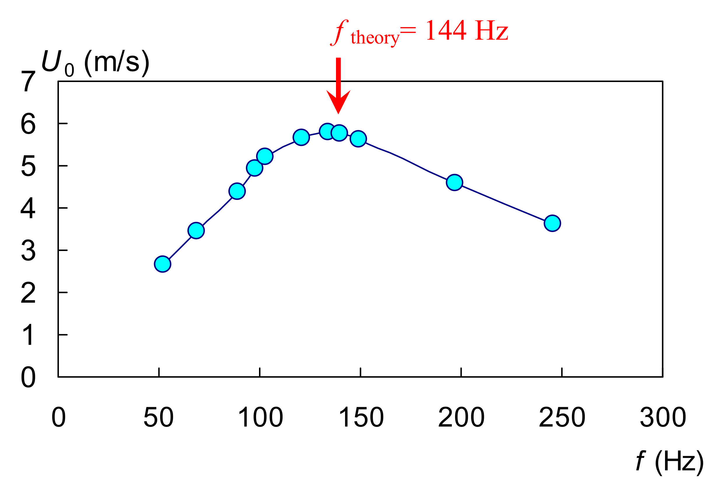
Figure 3 shows the velocity resonance curve as the dependence of the characteristic velocity on the driving frequency. The measurement was made for a constant real input power of P = 2.0 W ± 1%. The maximum U0 velocity was achieved approximately at 134 Hz.
The first resonance of the actuator results from a transformation between the potential energy of the diaphragm and the jet kinetic energy during each period. The first natural frequency can be derived theoretically [62] as
where ASJ and AD are the cross-sectional areas of the SJ actuator nozzle and the diaphragm [ASJ = π (Do2 − Di2)/4 and AD = π DD2/4, respectively], KP is the diaphragm spring constant, ρ is the working fluid (air) density, and Le is the effective “fluid column” length, Le = L1 + 8(Do − Di)/(3π). For the present geometry (Figure 2) and parameters of this study (ρ = 1.16 kg/m3, KP = 4.8 · 105 N/m3), Equation (3) yields ftheory = 144 Hz. This value is indicated by the arrow in Figure 3, showing a very good agreement with the experimental maximum of the velocity resonance curve.
3.2. Parameters of Examined Jets
Table 1 summarizes the parameters of the studied jets. Overall, 11 cases with Reynolds number of the main jet ranging Re = (1082–5181) were examined. The Reynolds numbers were chosen to cover the area of initially laminar, transitional, and turbulent flows. The initial character of the main jet can be described by the ratio of the maximum velocity in the nozzle exit profile (Umax, on the jet axis) and the mean exit velocity as follows:
k = Umax/Um.
The k of the laminar (nearly parabolic) profile is close to the value of 2, while the fully turbulent velocity profile (top hat) exhibits k around 1.2. It can be seen in Table 1 that the jet’s profile remains laminar (at the pipe exit) up to Re ≈ 2163; as Re further increases, the velocity profile then undergoes the gradual transition to turbulence.
For every case of the main (continuous) jet, the complementary synthetic jet was chosen. The parameters (the frequency and power input) of the SJ were chosen to keep the velocity ratio cu and Strouhal number approximately constant for all the cases. The velocity ratio was cu = 0.5, and the Strouhal number was kept close to the expected preferred mode of the main jet, i.e., approximately St = 0.3; see Crow and Champagne [5].
3.3. Velocity Fields
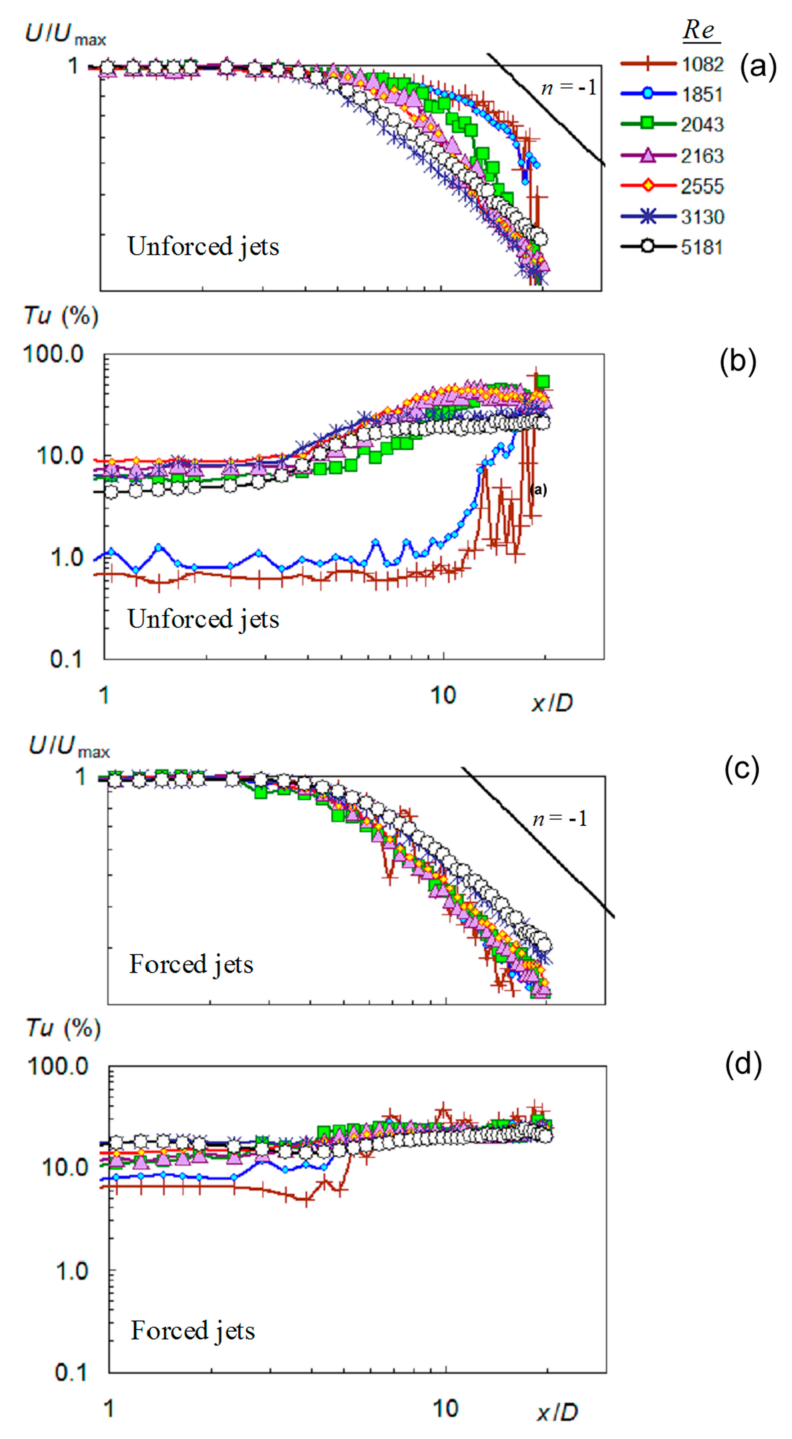
Axial velocity profiles of the selected unforced cases from Table 1 along the jet axis (r = 0) are shown in Figure 4a. The results are presented in the dimensionless form of U/Umax. With increasing Reynolds number from Re = 1082 to 5181, the jets undergo a transition from the laminar regime (Re = 1082–1851) to the turbulent regime (Re = 3130–5181). The jets with Re = 2043–2947 are the transitional ones. The region of the constant velocity indicates the potential core for x/D = 0–4. Farther downstream, the velocity decay is developed. For the laminar cases, the process is gradual, without a rapid turning point in the relationship. On the other hand, the turbulent cases show well distinguishable regions of the constant velocity (potential core for x/D < 4) and the exponential velocity decay with exponent approximately n = −1 for x/D > 4. The transitional cases represent the link between the laminar and turbulent behavior.
The laminar–turbulent transition is also evident from the corresponding development of the turbulence intensity, Tu = uRMS/U (Figure 4b), where uRMS is the fluctuation velocity and U is the time-mean velocity at the same point. The difference between the laminar and turbulent regimes is substantial: the level of Tu of laminar jets keeps under 1% up to the distance approximately x/D = 10, then it abruptly increases. In contrast, the level of Tu of the turbulent cases is higher from the very beginning, up to 10% in the jet potential core region and rising higher more downstream. At the end of the studied area (x/D ≈ 20), the levels of Tu in initially laminar and turbulent cases reach approximately the same level between 20% and 30%.
The increase in the Tu level in laminar cases indicates that up to this distance the jets undergo the transition to turbulence. The highest Tu level in the potential core region was observed for Re = 2820, and with further increased Re, the Tu level slightly decreases. The switching between the laminar and turbulent Tu curves occurs suddenly between Re = 1851 and 2043, and no interjacent curve was found. However, the end of the transitional process cannot be unambiguously evaluated from axial velocity, and its fluctuation because no noticeable difference was found between the transitional and turbulent velocity profiles.
The evolution of the axial velocity of the forced jets (the jet control is applied) is shown in Figure 4c, and the corresponding fluctuation velocity profiles are in Figure 4d. The forcing produces considerable changes in the jet flow. In all cases, the region of the constant velocity after the nozzle exit can be seen up to the distance x/D = 4; this potential core region is followed by the sharp decrease in velocity. While the forcing has almost no effect for the initially turbulent cases, the striking difference can be observed between the unforced and forced initially laminar cases (Re = 1082–1851), indicating that all the jets under the forcing became turbulent at some distance, see Figure 4a,c. The forcing also affects the intensity of turbulence. The forcing draws the Tu of the laminar cases nearer to the turbulent ones; however, it is still lower in the initial (potential core) region (between 2% and 5%). The maximum value of Tu here is achieved for Re = 2820 and 3130. A slight drop occurs at the end of the initial region for all the jets, this is again followed by an increase in the Tu level, less marked with increasing Re.
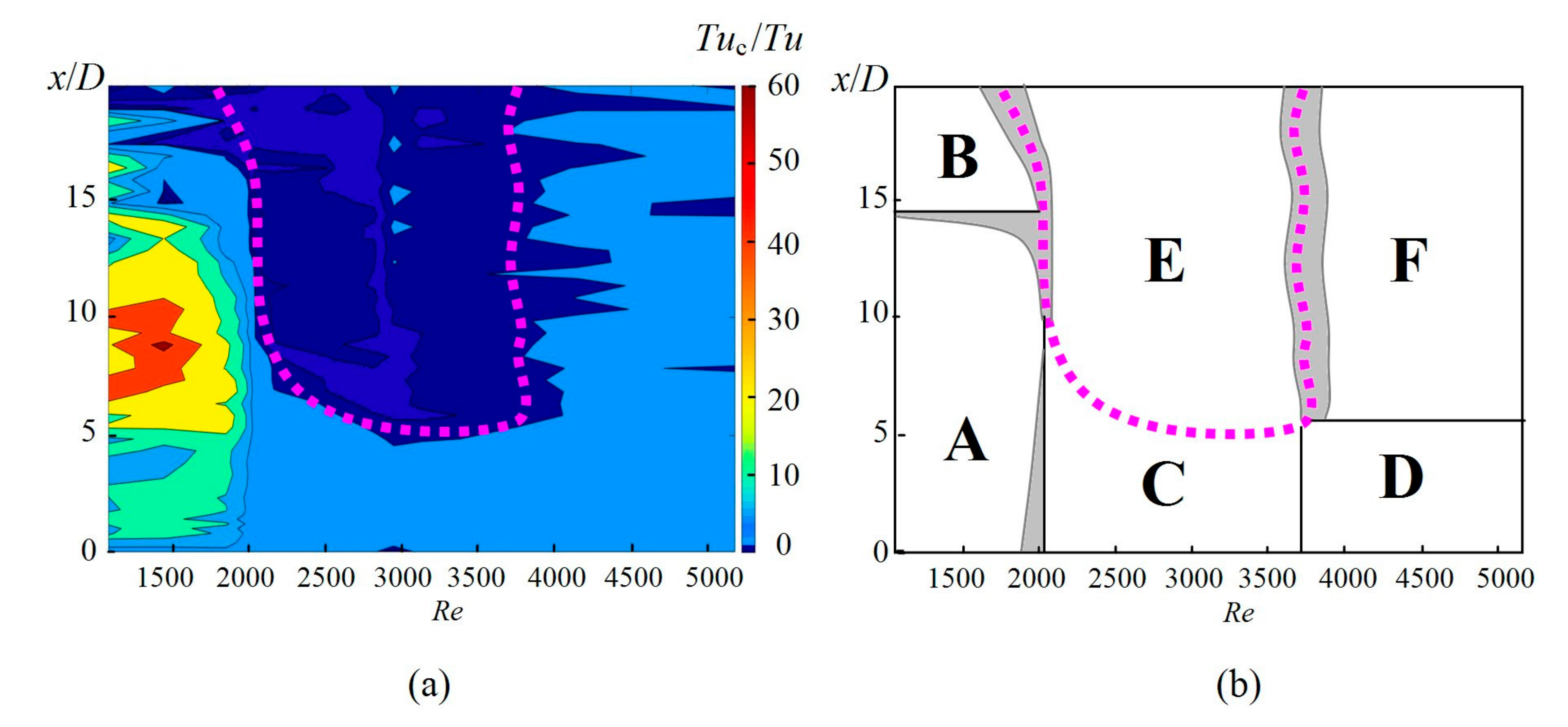
As expected, the control forcing impacts regimes of the main flow. For the given geometry and chosen parameters of the control SJ (cu = 0.5 and St = 0.3 for all experiments of this study), the local flow regime along the jet axis depends on two parameters: Re and x/D. Figure 5 shows a map of parameters related to the flow regimes. For each point along the jet axis, the Tuc/Tu ratio between the turbulent intensity in the forced and unforced cases was evaluated, and Figure 5a shows the dependency of Tuc/Tu on Re and x/D. Six flow regimes A–F were distinguished from Figure 5a; their basic parameters are listed in Table 2, and the occurrence of these regimes is presented in Figure 5b.
Initial region A has an enormous increase in the turbulence level in low Re jets. The region is located near the nozzle exit, in the jet core. The Tuc/Tu ratio achieves values of 2–67. The region occurs approximately for Re < 2043 and x/D < 14.5.
Intermediate region B has a turbulence increase in low Re jets. The region is located downstream the jet core, x/D > 14.5 for Re < 2043. The Tuc/Tu achieves values around 4.
Initial region C has weak or moderate turbulence increase in the core of transitional jets where Tuc/Tu = 1.3–1.9. The region occurs approximately for Re = 2000–3700 and x/D < 5–9.
Initial region D has a turbulence increase in the jet core of turbulent jets. The Tuc/Tu ratio is 1.5–2 for Re = 3700–5000.
Intermediate region E has a decrease in the turbulence level in transitional jets. The Tuc/Tu ratio is 0.45–1.0 and the region boundary defined by Tuc/Tu = 1 is plotted by the dotted curve in Figure 5a,b. The reason for the turbulence decrease lies in the promotion of the turbulence transition and acceleration of the energy transport process from the large-scale structures to the smaller ones. In forced jets, these processes proceed predominantly in the initial region C, which exists upstream of the E region.
Intermediate region F has a relatively weak increase or stagnation of the turbulence level, where Tuc/Tu = 0.9–1.2.
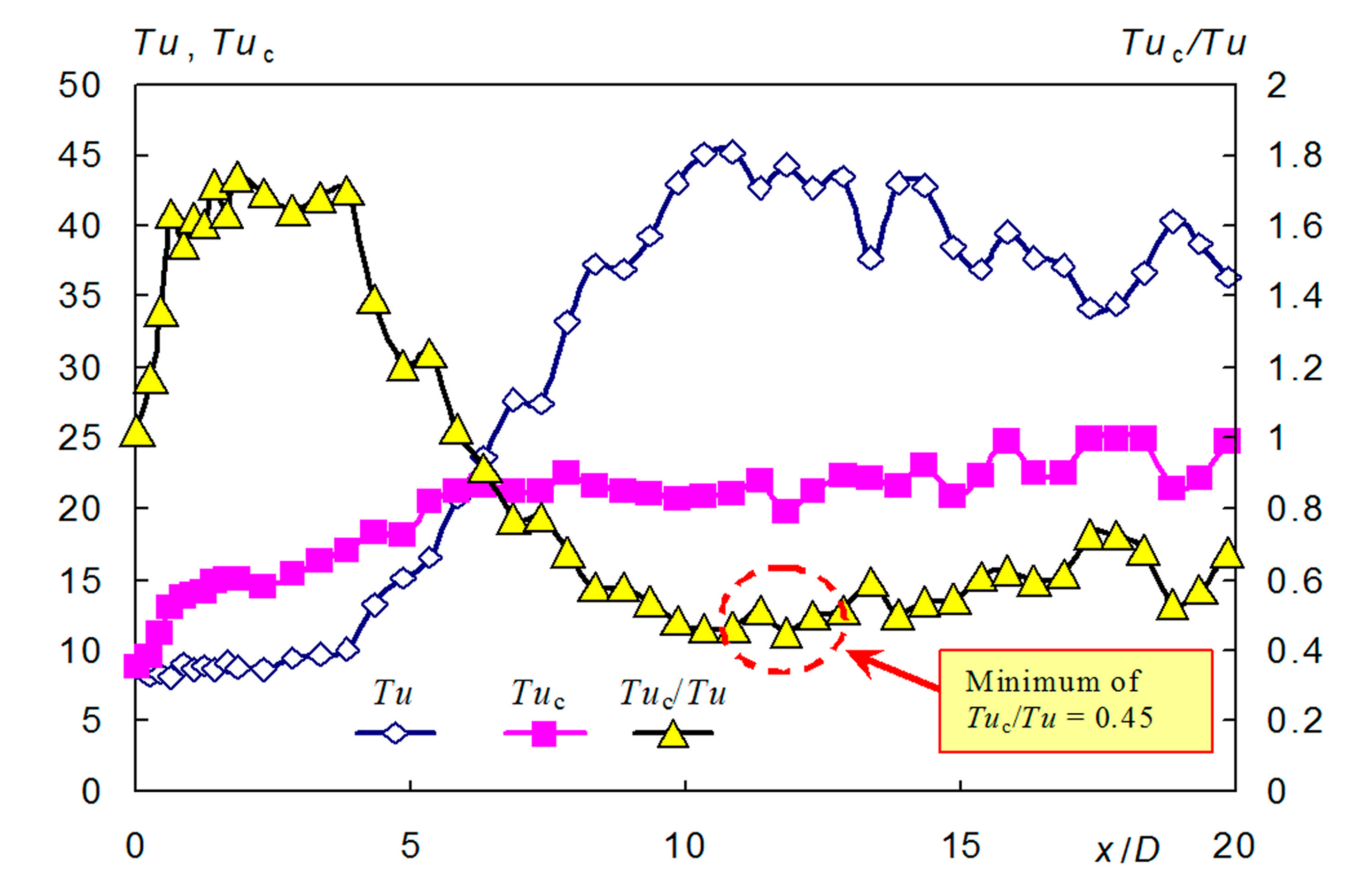
As the E flow regime with turbulence reduction by the flow control seems to be potentially interesting for subsequent investigations, a typical example of the development of the turbulence intensities is presented in Figure 6 for Re = 2555. Development of the Tuc/Tu ratio is plotted in Figure 6 as well, showing the minimum achieved ratio of Tuc/Tu = 0.45.
An intermittency factor γ was evaluated using a modification of the TERA method, see, e.g., [63]. The hot-wire velocity data were filtered to remove the noise, and the detection function was evaluated in the form of in MATLAB. As the next step, the Z(t) results were smoothed and the criterion function S(t) was applied, and the threshold was chosen as C = 10. Subsequently, to distinguish the turbulent and nonturbulent parts of the signal, the indicator function I(t) was used as follows:
I(t) = 1, when S(t) C for the turbulent part, I(t) = 0, when S(t) < C for the nonturbulent part.
Finally, the intermittency factor was evaluated.
where N is the number of samples.
The factor was evaluated at the nozzle axis (r = 0), closely downstream of the nozzle exit (x = 0.5 mm), and at x/D = 5. The γ-factor for both unforced and forced jets near the nozzle exit is presented in Figure 7a. The intermittency factor remains nearly zero for the Re = 1082–1851 near the nozzle exit, then starts to increase and approaches the value of 1 at Re = 4151, indicating completion of the transitional process. The onset of the transition well agrees with profiles of axial and fluctuation velocity components shown in Figure 4a,b, where the beginning of the transition was also identified at Re = 2043. The forcing influences the γ−factor, the curve of γ is shifted practically equidistantly toward the lower Reynolds numbers. The transition begins at Re = 1445 and is finished with Re = 2820. It is worth noting that the annular SJ is not fully merged so near the nozzle exit; despite this fact, the forcing affects considerably the main jet from the moment the jet exits the nozzle. This can be attributed to the effect of an acoustic excitation caused by the forcing jet. The intermittency factor of the unforced jet remains almost unchanged at x/D = 5; a slight increase is achieved in the transitional cases. However, the forcing causes the increase in the γ-factor for all the cases. Three, initially laminar, jets change into the transitional ones, and all the transitional jets become turbulent by this distance. To complete the picture, Figure 7b shows the intensities of turbulence of unforced and forced jets at the same positions as in Figure 7a. In all cases, the maximum occurs within the end of the transitional region (cf. Figure 7a).
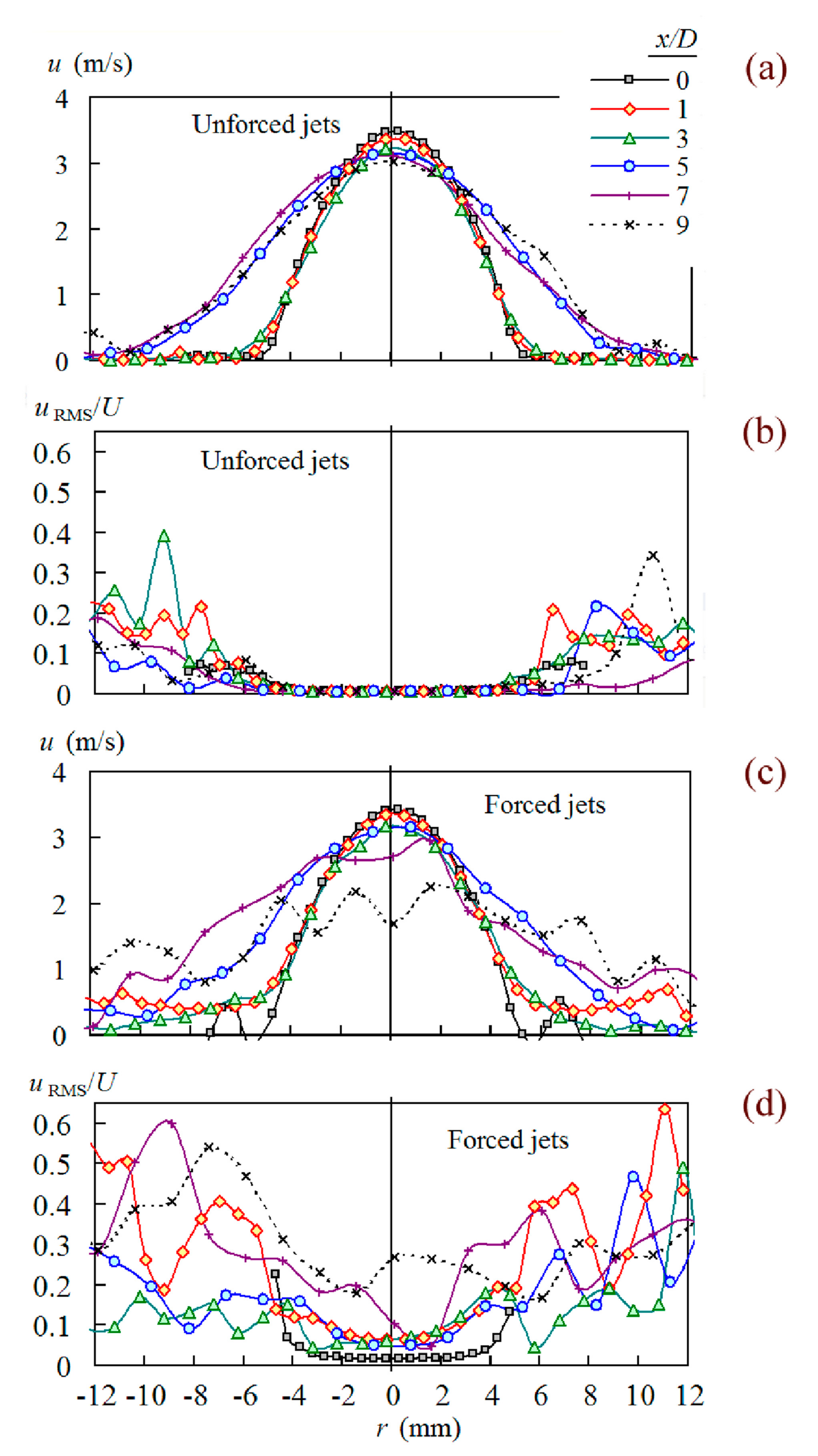
The effect of the forcing can be shown also on the transverse velocity profiles. Figure 8 shows the velocity and Tu profiles of the jet with Re = 1082 without forcing (Figure 8a,b) and with forcing (Figure 8c,d), respectively. In accord with the previous findings from Figure 3 and Figure 7, the initial velocity profile (x/D = 0) is typically laminar with a parabolic shape. The profiles remain almost unchanged up to x/D = 3. With increasing distance, the slight decrease in the axial velocity accompanied by the profiles’ widening can be seen in Figure 8a (see also Figure 4a). The level of turbulence intensity is low; see Figure 8b.
Forcing does not cause a substantial change to the nozzle exit velocity profile; the only difference is the addition of the control jet, visible as two side peaks in Figure 8c. With increasing distance, the control jet gradually merges with the main jet, and the profiles become wider. This is accompanied by axial velocity decay. Both the widening and axial velocity decay are faster than in the unforced case. The forcing also brings the changes in the Tu profiles; the Tu level increases in all the distances and in all the transverse positions.
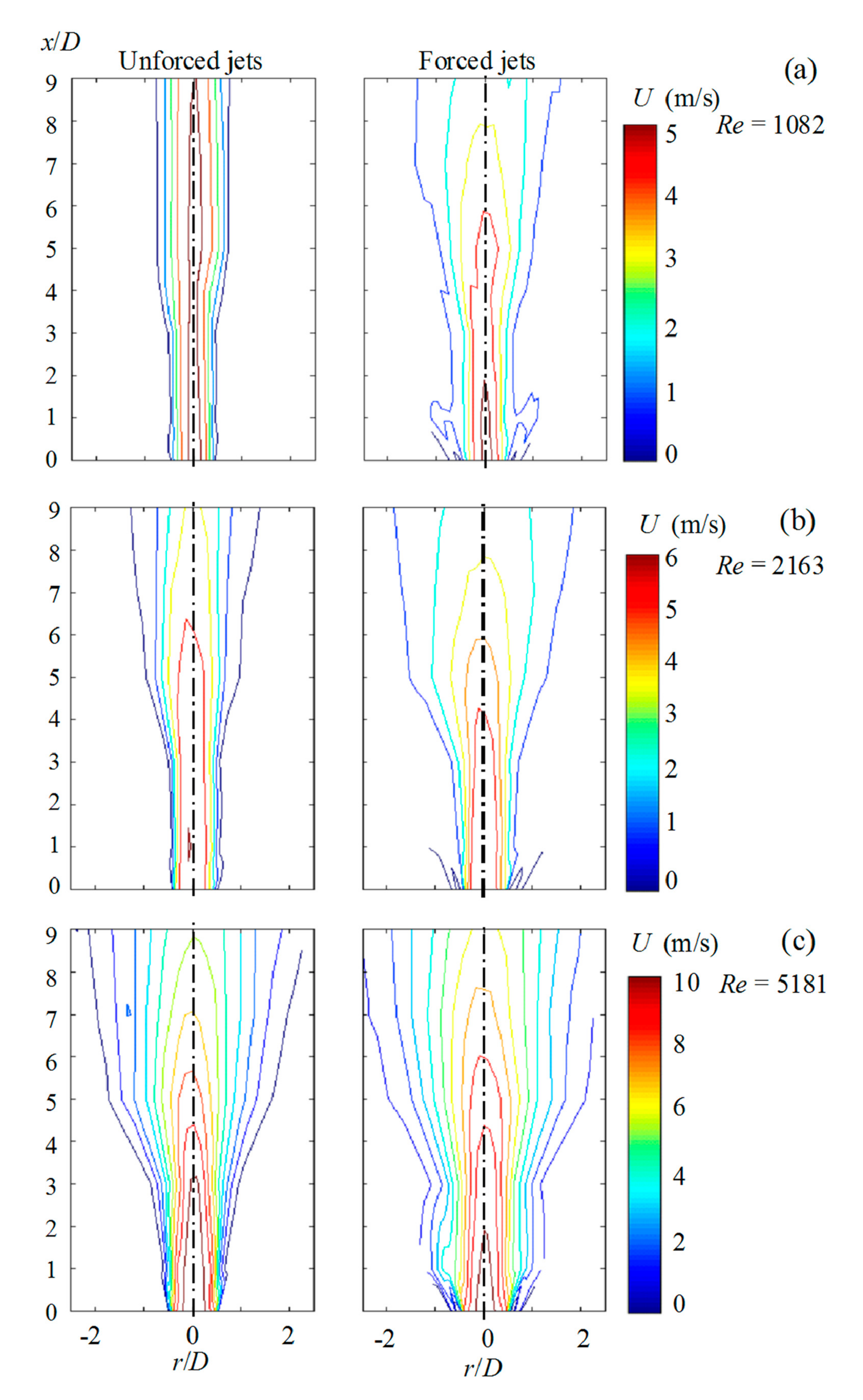
For illustration purposes, the velocity profiles from Figure 8a,c were transformed into the velocity maps shown in Figure 9a. The shortening of the potential core in the forced case is apparent, as well as the widening of the jet. The direct effect of the control SJ jet is mainly visible in the very nearfield where it causes the increase in the velocity at the sides of the main jet before it is fully merged. The merging is finished around x/D = 3.
Figure 9b shows the velocity maps of the jet with Re = 2163, i.e., jet from the transition regime, unforced and forced cases. The same data processing was made for Re = 5181 (turbulent regime), and the results are shown in Figure 9c. The effect of forcing on the velocity map (shortening of the potential core, widening of the jet) is apparent in both Figure 9b,c; however, with increasing Reynolds number, it is less prominent than that of the initially laminar case (Figure 9a, Re = 1851).
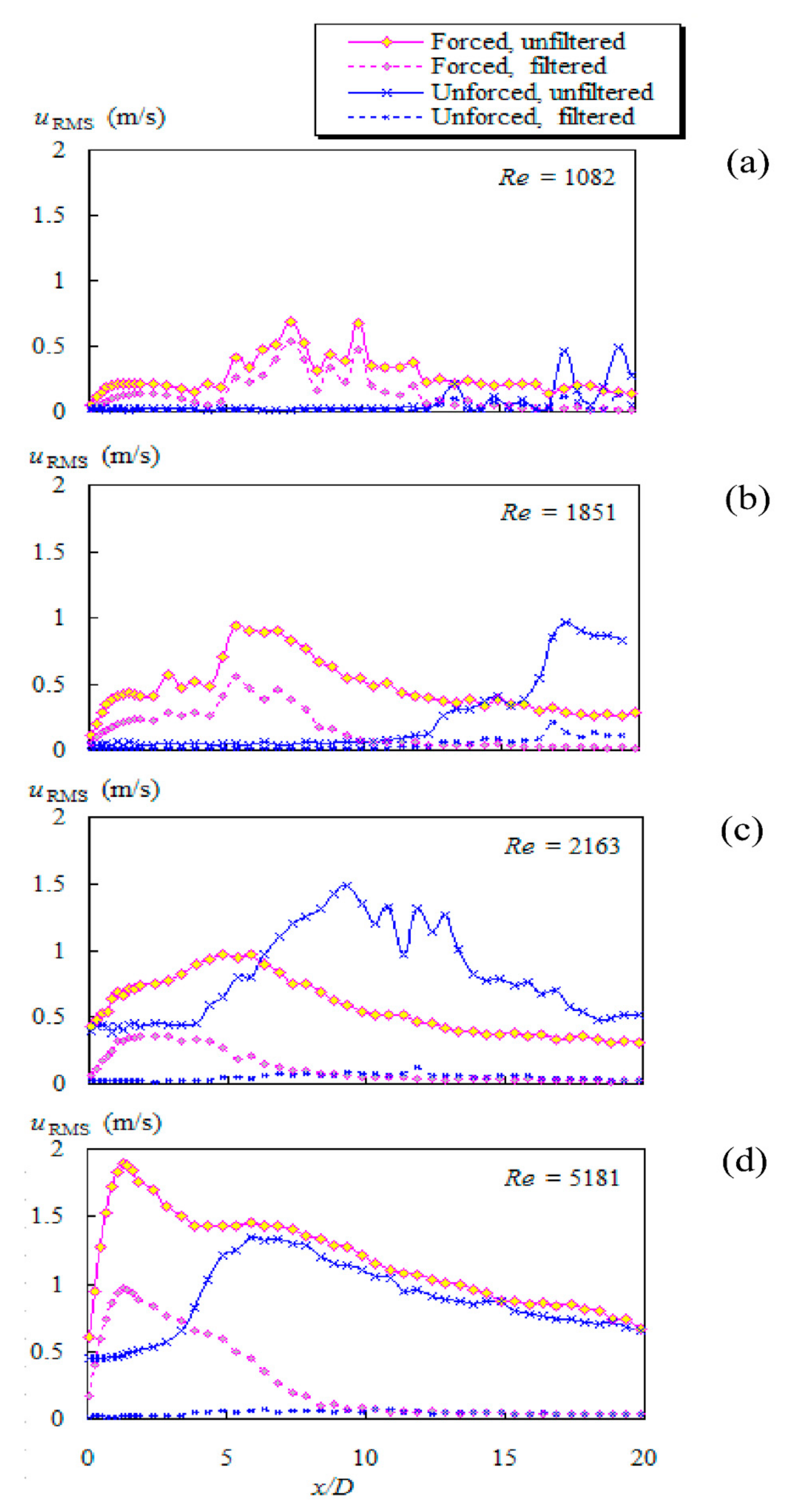
Following the approach of Crow and Champagne [5], the axial profiles of the velocity fluctuations of four selected forced cases (Re = 1082, 1851, 2163, and 5181) were filtered using Butterworth bandpass filter around the forcing frequency (St ≈ 0.3). The resultant filtered profiles are shown together with unfiltered profiles in Figure 10. For comparison purposes, profiles of the corresponding unforced jets are plotted as well. The influence of the forcing frequency is apparent mainly in the near nozzle-exit region where the large-scale eddies dominate.
In low Re jets at Re = 1082 and 1851, the dominance of the large-scale structures relating to the forcing frequency in the near nozzle-exit region is indicated by the local maximum around x/D = 1.7–2.5. Further downstream, both filtered and unfiltered fluctuations increase abruptly again. The beginning of the second rise corresponds to the onset of velocity decay at x/D = 4.4, i.e., shortly beyond the tip of the potential core (see Figure 4c). The large-scale structures relevant to the forcing frequency fade away more downstream of x/D > 15 and 12 for Re = 1082 and 1851, respectively.
For the transitional and turbulent jets (Re = 2163 and 5181, respectively), the maximum in the filtered profiles can be found around x/D = 3 and x/D = 2, respectively. Further downstream, the dominance of the large eddies corresponding to the forcing frequency weakens and the influence totally diminishes up to x/D = 10. Correspondingly to this fact, no dominant peak was identified in the PSD distributions beyond x/D = 10 for investigated transitional and turbulent jets.
Finally, a commensurable behavior revealing the maximum velocity fluctuations near the nozzle exit was discussed in literature dealing with the forced jets. Similar to the present findings, the maxima were attributed to the large-scale structures relating to the forcing frequency, as was observed in turbulent jets, see, e.g., Crow and Champagne [5] around x/D = 4 and Lepičovský et al. [17] around x/D = 3.
3.4. Power Spectral Density of Velocity Fluctuations
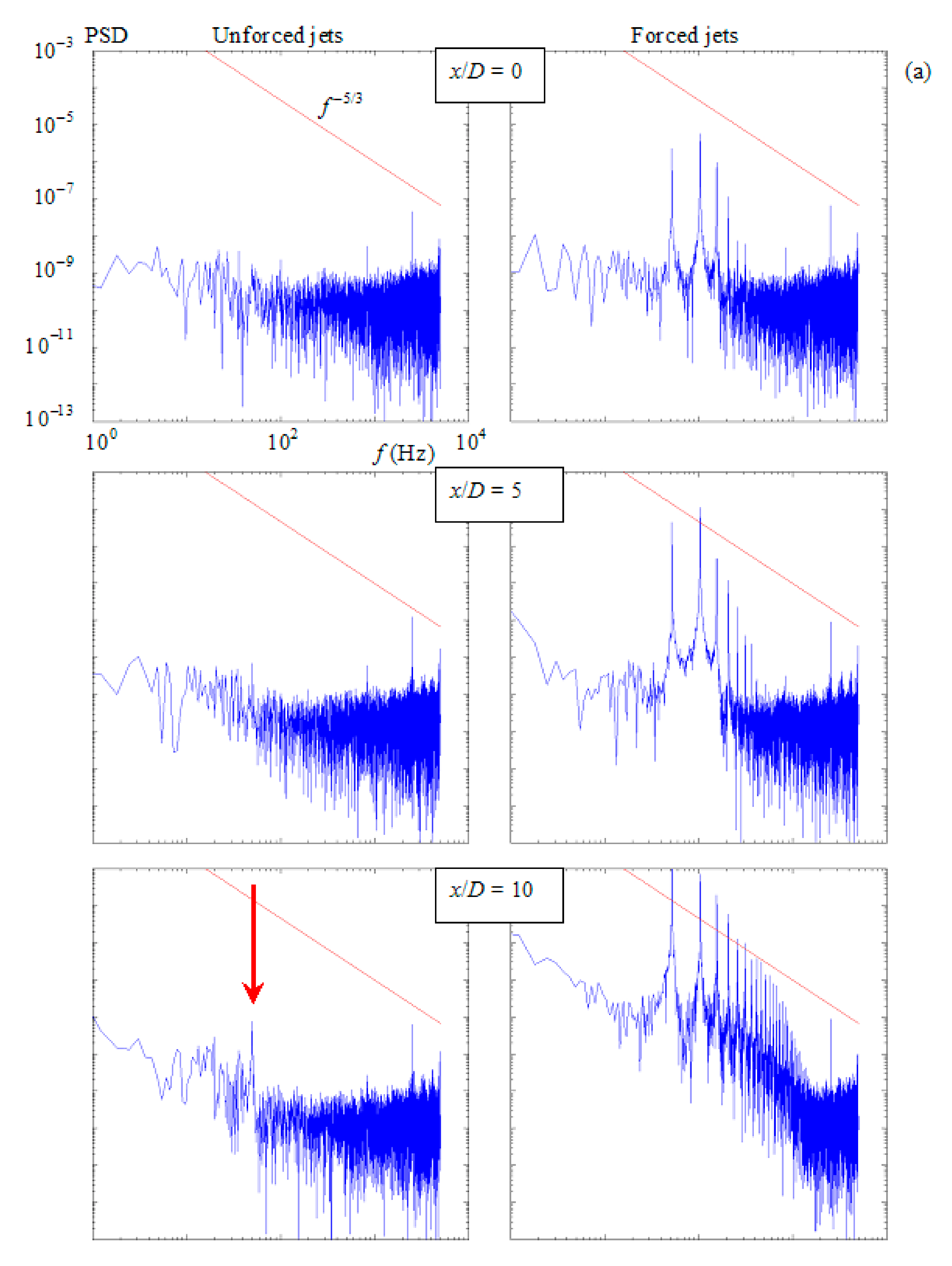
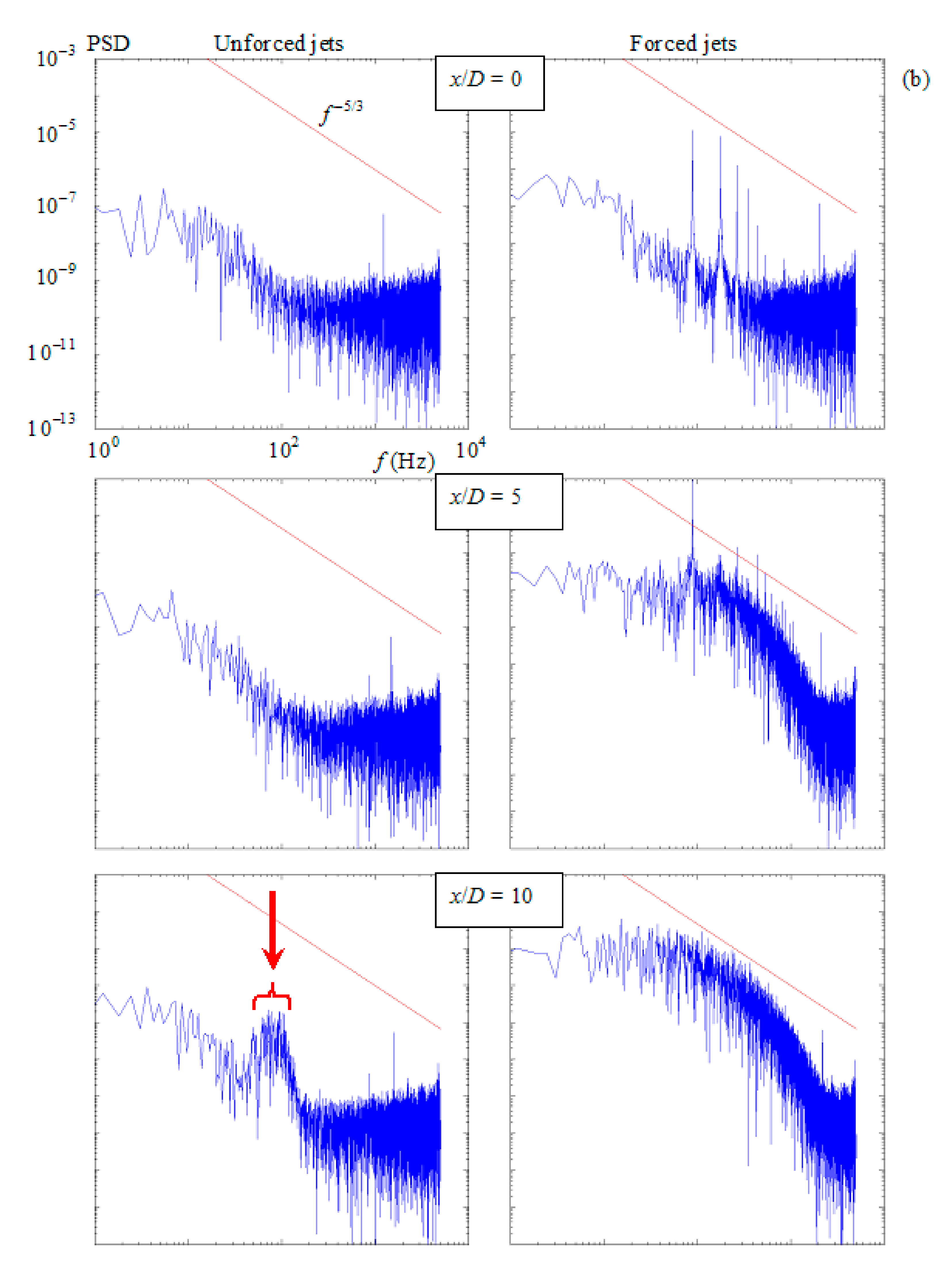
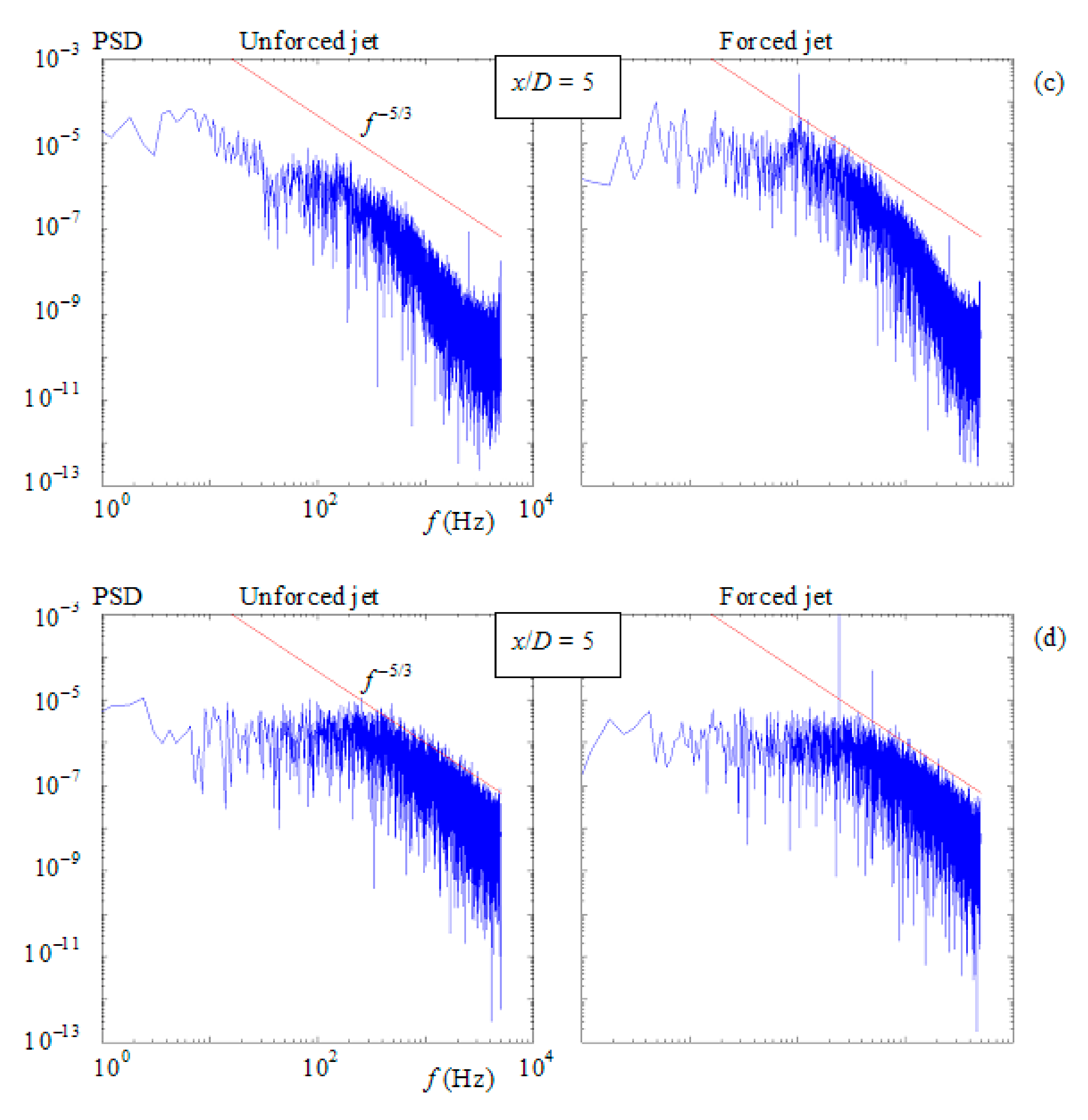
The power spectral density (PSD) distributions of velocity fluctuations were evaluated at three locations on the axis: x/D = 0, 5, and 10, i.e., at the nozzle exit, shortly downstream the potential core tip and in the velocity decay region, both for the unforced and forced cases.
3.4.1. Unforced Jets
In Figure 11a, PSDs of the jet with Re = 1082 are shown. The overall PSD level of the laminar unforced jet is low when compared with transitional and turbulent cases, the PSD distribution remains practically unchanged at all studied distances. For the unforced jet at x/D = 10, a peak of a natural frequency of the jet column large eddy structures can be identified at approximately 52 Hz, i.e., St = 0.3, see the arrow in Figure 11a. This value corresponds well to the natural frequency observed by, e.g., Crow and Champagne [5].
A similar behavior can be seen for the Re = 1851 (Figure 11b). It is worth noting that not only one singular dominant frequency is visible for this Reynolds number for the unforced jet but the larger region at the spectrum is also increased at x/D = 10, namely, St = 0.17–0.40; see the arrow in Figure 11b.
When the Reynolds number is increased towards the transitional regime (unforced case), and the PSD level is increased as well; see Figure 11c for Re = 2163 and x/D = 5. Moreover, the distribution begins to form the slope with Kolmogorov’s exponent −5/3, which is a typical demonstration of the energy cascade of fully developed turbulent flows. However, the development is not finished yet, as is evident from Figure 11c, because the PSD distribution still does not obey the slope relating to the exponent −5/3. For illustration purposes, the line relating to Kolmogorov’s exponent −5/3 is plotted in Figure 11 as well. Note that the dominant frequency cannot be identified in Figure 11c, unlike Figure 11a,b.
The turbulent unforced jet with Re = 5181 has already fully developed a cascade of energy transport at the distance of x/D = 5, which is indicated by the PSD distribution with the slope relating to the exponent −5/3; see Figure 11d. Similar to the case presented in Figure 11c, the dominant frequency cannot be identified in Figure 11d.
3.4.2. Forced Jets
When the jet control is applied, the power spectra of all the cases undergo a change. The most dramatic transformation can be observed in the initial laminar cases (Figure 11a,b). For Re = 1082, the massive peaks of the forcing frequency and its harmonics dominate the spectrum. The further the distance x is, the more peaks of harmonics are detectable. Although the overall PSD level slowly increases, the peaks remain discrete, and they do not merge in one high-level spectral distribution. It indicates that the jet is disturbed but the level of the excitation is not high enough to cause the transition to turbulence up to the present distance of x/D = 10. A slightly different situation comes about for the faster but still laminar jet with Re = 1851 (Figure 11b). In the very exit region, a cascade of discrete peaks of the forcing frequency, and its harmonics dominate the spectrum, which is a similar behavior, as shown in Figure 11a. However, further downstream (x/D = 10), the overall level of the PSD distribution increases, the discrete peaks from forcing slowly diminish, and the spectrum begins to form the slope of the turbulent energy spectrum, indicating the transition to turbulence.
The spectra of transitional and turbulent forced jets do not differ much from the unforced ones (Figure 11c,d). The main difference is the presence of the discrete peaks of the forcing frequencies and their harmonics. In the transitional case shown in Figure 11c, the forcing causes a slight increase in the PSD level. In the turbulent case (Figure 11d), the overall level remains practically unchanged, and the PSD distribution well obeys the slope relating to Kolmogorov’s exponent −5/3.
4. Conclusions
Continuous jet issuing from a long straight circular pipe (pipe nozzle in short) was actively controlled using a concentrically placed annular synthetic jet. The range of Reynolds numbers of the main jet covers the area of laminar, transitional, and turbulent jets (Re = 1082–5181). The control parameters, i.e., the Strouhal number and ratio of the control and main jet velocities, were kept constant, at 0.5 and 0.3, respectively. Flow velocities were measured using a hot-wire anemometer. The power spectral density (PSD) distributions of velocity fluctuations were evaluated from the hot-wire data. The presence of large-scale structures related to the control jet was manifested.
The possibility of the control by means of the annular synthetic jet was proven. It was revealed that forcing increases the intermittency factor and thus accelerates the transition to turbulence. It also leads to the reduction of the potential core of the main jet. Based on the hot-wire data, six flow regimes of the controlled jets were identified, and their parameter map was proposed.
Finally, the turbulence intensity decrease was obtained in the specific region called E in the paper. The maximal effect was revealed at Re = 2555, when the turbulence intensity of the unforced jet was 44.4% at the distance of 12 diameters of the pipe nozzle, while the jet control decreased to the value of 19.9%, i.e., the ratio of the turbulence intensities of the forced and unforced jets was 0.45 in this case.
The results are considered as important for jet flow research in general, with a potential for various applications, of which the actively controlled impinging jet intended for convective heat transfer augmentation is an example.
Author Contributions
Conceptualization, Z.A. and Z.T.; funding acquisition, Z.T.; investigation, Z.A.; methodology, Z.A. and Z.T.; project administration, Z.A. and Z.T.; software, Z.A.; supervision, Z.A. and Z.T.; writing—original draft preparation, Z.A. and Z.T.; writing—review and editing, Z.A. and Z.T. Both authors have read and agreed to the published version of the manuscript.
Funding
This research was funded by the Grant Agency of the Czech Republic—Czech Science Foundation (Project No. 21-26232J).
Institutional Review Board Statement
Not applicable.
Informed Consent Statement
Not applicable.
Data Availability Statement
Not applicable.
Acknowledgments
The experiments were performed at the Institute of Thermomechanics of the Czech Academy of Sciences in Prague, Czech Republic. We gratefully acknowledge the institutional support (RVO:61388998).
Conflicts of Interest
The authors declare no conflict of interest.
Nomenclature
| B | width of the annular slot, B = (Do − Di)/2 |
| Di | inner diameter of annular nozzle |
| Do | outer diameter of annular nozzle |
| f | driving frequency (Hz) |
| k | velocity ratio, k = Umax/Um |
| r | radial coordinate, see Figure 1 and Figure 2 |
| Re | Reynolds number of round jet, Re = Um D/ν |
| ReSJ | Reynolds number of control SJ, ReSJ = U0Do/ν |
| SJ | synthetic jet |
| t | time |
| T | time period, T = 1/f |
| Tu | turbulence intensity, Tu = uRMS/U |
| uRMS | fluctuation velocity, (m/s) |
| u0 | velocity of the SJ at the nozzle exit, x = 0 |
| U | time-mean velocity, (m/s) |
| U0 | time-mean orifice velocity of SJ, see Equation (1) |
| Um | mean exit velocity of the main jet, (m/s) |
| Umax | maximum velocity in the exit profile of the main round jet, (m/s) |
| x | axial coordinate, see Figure 1 and Figure 2 |
| ν | kinematic viscosity of the working fluid (air) |
| ρ | density of the working fluid (air) |
| γ | intermittency factor |
References
- Schlichting, H. Boundary-Layer Theory; McGraw Hill: New York, NY, USA, 1955. [Google Scholar]
- Abramovich, G.N. The Theory of Turbulent Jets; The MitPress: Cambridge, MA, USA, 2003. [Google Scholar] [CrossRef]
- Blevins, R.D. Applied Fluid Dynamics Handbook; Krieger Publishing: Malabar, FL, USA, 2003. [Google Scholar]
- Bejan, A. Convection Heat Transfer; Wiley Interscience Publication: New York, NY, USA, 1995. [Google Scholar]
- Crow, S.C.; Champagne, F.H. Orderly structure in jet turbulence. J. Fluid Mech. 1971, 48, 547–591. [Google Scholar] [CrossRef]
- Yule, A.J. Large-scale structure in the mixing layer of a round jet. J. Fluid Mech. 1978, 89, 413–432. [Google Scholar] [CrossRef]
- Hussain, A.K.M.F.; Husain, H.S. Passive and active control of jet turbulence. In Turbulence Management and Relaminarisation; Liepmann, H.W., Narasimha, R., Eds.; Springer: Berlin/Heidelberg, Germany, 1988. [Google Scholar]
- Zaman, K.B.M.Q. Axis switching and spreading of an asymmetric jet: The role of coherent structure dynamics. J. Fluid Mech. 1996, 316, 1–27. [Google Scholar] [CrossRef]
- Komori, S.; Ueda, H. The large-scale coherent structure in the intermittent region of the self-preserving round free jet. J. Fluid Mech. 1985, 152, 337–359. [Google Scholar] [CrossRef]
- Thomas, F.O. Structure of mixing layers and jets. Appl. Mech. Rev. 1991, 44, 119–153. [Google Scholar] [CrossRef]
- Matsuda, T.; Sakakibara, J. On the vortical structure in a round jet. Phys. Fluids 2005, 17, 25106. [Google Scholar] [CrossRef] [Green Version]
- Fiedler, H.; Fernholz, H.-H. On management and control of turbulent shear flows. Prog. Aerosp. Sci. 1990, 27, 305–387. [Google Scholar] [CrossRef]
- Gad-el-Hak, M. Modern developments in flow control. Appl. Mech. Rev. 1996, 49, 365–379. [Google Scholar] [CrossRef]
- Liu, T.; Sullivan, J. Heat transfer and flow structures in an excited circular impinging jet. Int. J. Heat Mass Transf. 1996, 39, 3695–3706. [Google Scholar] [CrossRef]
- Kibens, V. Discrete noise spectrum generated by acoustically excited jet. AIAA J. 1980, 18, 434–441. [Google Scholar] [CrossRef]
- Vlasov, E.V.; Ginevskii, A.S. The aeroacoustic interaction problem. Sov. Phys. Acoust. 1980, 26, 1–7. [Google Scholar]
- Lepičovský, J.K.K.; Ahuja, R.H.; Burrin, R.H. Tone excited jets, part III: Flow measurements. J. Sound Vibr. 1985, 102, 71–91. [Google Scholar] [CrossRef]
- Cho, S.K.; Yoo, J.Y.; Choi, H. Vortex pairing in an axisymmetric jet using two-frequency acoustic forcing at low to moderate strouhal numbers. Exp. Fluids 1998, 25, 305–315. [Google Scholar] [CrossRef]
- Vejrazka, J.; Tihon, J.; Marty, P.; Sobolík, V. Effect of an external excitation on the flow structure in a circular impinging jet. Phys. Fluids 2005, 17, 105102. [Google Scholar] [CrossRef] [Green Version]
- Hwang, S.; Lee, C.; Cho, H. Heat transfer and flow structures in axisymmetric impinging jet controlled by vortex pairing. Int. J. Heat Fluid Flow 2001, 22, 293–300. [Google Scholar] [CrossRef]
- Diep, J.; Sigurdson, L. Cross-jet influenced by a concentric synthetic jet. Phys. Fluids 2001, 13, S16. [Google Scholar] [CrossRef] [Green Version]
- Koso, T.; Kinoshita, T. agitated turbulent flowfield of a circular jet with an annular synthetic jet actuator. J. Fluid Sci. Technol. 2008, 3, 323–333. [Google Scholar] [CrossRef] [Green Version]
- Smith, B.L.; Glezer, A. The formation and evolution of synthetic jets. Phys. Fluids 1998, 10, 2281–2297. [Google Scholar] [CrossRef]
- Mallinson, S.G.; Reizes, J.A.; Hong, G. An experimental and numerical study of synthetic jet flow. Aeronaut. J. 2001, 105, 41–49. [Google Scholar] [CrossRef]
- Glezer, A.; Amitay, M. Synthetic jets. Annu. Rev. Fluid Mech. 2002, 34, 503–529. [Google Scholar] [CrossRef]
- Mohseni, K.; Mittal, R. Synthetic Jets, Fundamentals and Applications; CRC Press Taylor & Francis: Boca Raton, FL, USA, 2015. [Google Scholar]
- Pack, L.G.; Seifert, A. periodic excitation for jet vectoring and enhanced spreading. J. Aircr. 2001, 38, 486–495. [Google Scholar] [CrossRef] [Green Version]
- Cater, J.E.; Soria, J. The evolution of round zero-net-mass-flux jets. J. Fluid Mech. 2002, 472, 167–200. [Google Scholar] [CrossRef]
- Dauphinee, T.M. Acoustic air pump. Rev. Sci. Instrum. 1957, 28, 456. [Google Scholar] [CrossRef]
- Gallas, Q.; Holman, R.; Nishida, T.; Carroll, B.; Sheplak, M.; Cattafesta, L. Lumped element modeling of piezoelectric-driven synthetic jet actuators. AIAA J. 2003, 41, 240–247. [Google Scholar] [CrossRef] [Green Version]
- Holman, R.; Utturkar, Y.; Mittal, R.; Smith, B.L.; Cattafesta, L. Formation criterion for synthetic jets. AIAA J. 2005, 43, 2110–2116. [Google Scholar] [CrossRef] [Green Version]
- Zhou, J.; Tang, H.; Zhong, S. Vortex roll-up criterion for synthetic jets. AIAA J. 2009, 47, 1252–1262. [Google Scholar] [CrossRef]
- Trávníček, Z.; Broučková, Z.; Kordík, J. Formation criterion for axisymmetric synthetic jets at high stokes numbers. AIAA J. 2012, 50, 2012–2017. [Google Scholar] [CrossRef]
- De Luca, L.; Girfoglio, M.; Coppola, G. Modeling and experimental validation of the frequency response of synthetic jet actuators. AIAA J. 2014, 52, 1733–1748. [Google Scholar] [CrossRef]
- Greco, C.S.; Cardone, G.; Soria, J. On the behaviour of impinging zero-net-mass-flux jets. J. Fluid Mech. 2016, 810, 25–59. [Google Scholar] [CrossRef]
- Gilarranz, J.L.; Traub, L.W.; Rediniotis, O.K. A new class of synthetic jet actuators—Part I: Design, fabrication and bench top characterization. J. Fluids Eng. Trans. ASME 2005, 127, 367–376. [Google Scholar] [CrossRef]
- Trávníček, Z.; Vít, T.; Tesař, V. Hybrid synthetic jet as the non-zero-net-mass-flux jet. Phys. Fluids 2006, 18, 081701-1–081701-4. [Google Scholar] [CrossRef]
- Yang, A.S.; Ro, J.J.; Yang, M.T.; Chang, W.H. Investigation of piezoelectrically generated synthetic jet flow. J. Vis. 2009, 12, 9–16. [Google Scholar] [CrossRef]
- Wang, J.; Shan, R.; Zhang, C.; Feng, L. Experimental investigation of a novel two-dimensional synthetic jet. Eur. J. Mech. B/Fluids 2010, 29, 342–350. [Google Scholar] [CrossRef]
- Kordík, J.; Travnicek, Z. Optimal diameter of nozzles of synthetic jet actuators based on electrodynamic transducers. Exp. Therm. Fluid Sci. 2017, 86, 281–294. [Google Scholar] [CrossRef]
- Smith, B.L.; Glezer, A. Jet vectoring using synthetic jets. J. Fluid Mech. 2002, 458, 1–34. [Google Scholar] [CrossRef]
- Mittal, R.; Rampunggoon, P. On the virtual aeroshaping effect of synthetic jets. Phys. Fluids 2002, 14, 1533–1536. [Google Scholar] [CrossRef] [Green Version]
- Amitay, M.; Glezer, A. Controlled transients of flow reattachment over stalled airfoils. Int. J. Heat Fluid Flow 2002, 23, 690–699. [Google Scholar] [CrossRef]
- Tensi, J.; Boué, I.; Paillé, F.; Dury, G. Modification of the wake behind a circular cylinder by using synthetic jets. J. Vis. 2002, 5, 37–44. [Google Scholar] [CrossRef]
- Ben Chiekh, M.; Béra, J.-C.; Sunyach, M. Synthetic jet control for flows in a diffuser: Vectoring, spreading and mixing enhancement. J. Turbul. 2003, 4, 32. [Google Scholar]
- Zhong, S.; Millet, F.; Wood, N.J. The behaviour of circular synthetic jets in a laminar boundary layer. Aeronaut. J. 2005, 109, 461–470. [Google Scholar] [CrossRef]
- Hong, G. Effectiveness of micro synthetic jet actuator enhanced by flow instability in controlling laminar separation caused by adverse pressure gradient. Sens. Actuators A Phys. 2006, 132, 607–615. [Google Scholar] [CrossRef] [Green Version]
- Tamburello, D.A.; Amitay, M. Three-dimensional interactions of a free jet with a perpendicular synthetic jet. J. Turbul. 2007, 8, N38. [Google Scholar] [CrossRef]
- Yassour, Y.; Stricker, J.; Wolfshtein, M. Heat transfer from a small pulsating jet. In Proceedings of the International Heat Transfer Conference, San Francisco, CA, USA, 17–22 August 1986. [Google Scholar] [CrossRef]
- Kercher, D.S.; Lee, J.-B.; Brand, O.; Allen, M.G.; Glezer, A. Microjet cooling devices for thermal management of electronics. IEEE Trans. Compon. Packag. Technol. 2003, 26, 359–366. [Google Scholar] [CrossRef]
- Trávníček, Z.; Tesař, V. Annular synthetic jet used for impinging flow mass–transfer. Int. J. Heat Mass Transf. 2003, 46, 3291–3297. [Google Scholar] [CrossRef] [Green Version]
- Gillespie, M.B.; Black, W.Z.; Rinehart, C.; Glezer, A. Local convective heat transfer from a constant heat flux flat plate cooled by synthetic air jets. J. Heat Transf. 2006, 128, 990–1000. [Google Scholar] [CrossRef]
- Arik, M. An investigation into feasibility of impingement heat transfer and acoustic abatement of meso scale synthetic jets. Appl. Therm. Eng. 2007, 27, 1483–1494. [Google Scholar] [CrossRef]
- Valiorgue, P.; Persoons, T.; McGuinn, A.; Murray, D. Heat transfer mechanisms in an impinging synthetic jet for a small jet-to-surface spacing. Exp. Therm. Fluid Sci. 2009, 33, 597–603. [Google Scholar] [CrossRef] [Green Version]
- Mangate, L.D.; Chaudhari, M.B. Experimental study on heat transfer characteristics of a heat sink with multiple-orifice synthetic jet. Int. J. Heat Mass Transf. 2016, 103, 1181–1190. [Google Scholar] [CrossRef]
- Persoons, T.; McGuinn, A.; Murray, D.B. A general correlation for the stagnation point Nusselt number of an axisymmetric impinging synthetic jet. Int. J. Heat Mass Transf. 2011, 54, 3900–3908. [Google Scholar] [CrossRef]
- Lee, A.; Yeoh, G.; Timchenko, V.; Reizes, J. Heat transfer enhancement in micro-channel with multiple synthetic jets. Appl. Therm. Eng. 2012, 48, 275–288. [Google Scholar] [CrossRef]
- Trávníček, Z.; Antošová, Z. Impingement heat transfer to the synthetic jet issuing from a nozzle with an oscillating cross section. Int. J. Therm. Sci. 2020, 153, 106349. [Google Scholar] [CrossRef]
- Silva-Llanca, L.; Ortega, A. Vortex dynamics and mechanisms of heat transfer enhancement in synthetic jet impingement. Int. J. Therm. Sci. 2017, 112, 153–164. [Google Scholar] [CrossRef]
- Broučková, Z.; Trávníček, Z.; Vit, T. Synthetic and continuous jets impinging on a circular cylinder. Heat Transf. Eng. 2018, 40, 1111–1125. [Google Scholar] [CrossRef] [Green Version]
- Broučková, Z. Active Control of the Jet Flow in Coaxial Arrangement. Master’s Thesis, Czech Technical University, Prague, Czech Republic, 2012. (In Czech). [Google Scholar]
- Trávníček, Z.; Fedorchenko, A.I.; Wang, A.-B. Enhancement of synthetic jets by means of an integrated valve-less pump, Part I: Design of the actuator. Sens. Actuators A Phys. 2005, 120, 232–240. [Google Scholar] [CrossRef]
- Falco, R.E.; Gendrich, C.P. The turbulence burst detection algorithm of Z. Zaric. In Proceedings of the 1988 Zoltan Zaric Memorial Conference on Near-Wall Turbulence, Dubrovnik, Yugoslavia, May 1988; Kline, S., Afgan, N.H., Eds.; Hemisphere Publishing Corp.: New York, NY, USA, 1990; pp. 911–931. Available online: https://ui.adsabs.harvard.edu/abs/1990nrw..book..911F/abstract (accessed on 20 June 2021).
Figure 1.
Schematic view on the studied coaxial jets.

Figure 2.
Investigated configuration (drawing not to scale); dimensions: φ D = 10.05 mm; Di = 11.95 mm; φ Di = 15.05 mm; L1 = 12.5 mm; L = 750 mm.
Figure 2.
Investigated configuration (drawing not to scale); dimensions: φ D = 10.05 mm; Di = 11.95 mm; φ Di = 15.05 mm; L1 = 12.5 mm; L = 750 mm.

Figure 3.
Frequency characteristics of the SJ actuator evaluated for P = 2.0 W.

Figure 4.
Axial velocity profiles of (a,b) unforced jets and (c,d) forced jets; (a,c) dimensionless time-mean velocity components, (b,d) turbulence intensities. For better clarity, the data set was plotted in a reduced version.
Figure 4.
Axial velocity profiles of (a,b) unforced jets and (c,d) forced jets; (a,c) dimensionless time-mean velocity components, (b,d) turbulence intensities. For better clarity, the data set was plotted in a reduced version.

Figure 5.
Map of parameters related to the flow regimes A to F evaluated along the jet axis: (a) the Tuc/Tu ratio; (b) demarcations of the flow regimes A to F.
Figure 5.
Map of parameters related to the flow regimes A to F evaluated along the jet axis: (a) the Tuc/Tu ratio; (b) demarcations of the flow regimes A to F.

Figure 6.
Development of the intensity of turbulence along the axis for Re = 2555 for unforced (Tu) and forced (Tuc) cases.
Figure 6.
Development of the intensity of turbulence along the axis for Re = 2555 for unforced (Tu) and forced (Tuc) cases.

Figure 7.
Jet quantities evaluated at x/D = 0.05 and 5 for Re = 1081–5181: (a) intermittency factor; (b) intensity of turbulence.
Figure 7.
Jet quantities evaluated at x/D = 0.05 and 5 for Re = 1081–5181: (a) intermittency factor; (b) intensity of turbulence.

Figure 8.
Radial profiles of time-mean velocity components and turbulence intensities at Re = 1082 for (a,b) unforced jets and (c,d) forced jets; (a,c) time-mean velocity components; (b,d) turbulence intensities.
Figure 8.
Radial profiles of time-mean velocity components and turbulence intensities at Re = 1082 for (a,b) unforced jets and (c,d) forced jets; (a,c) time-mean velocity components; (b,d) turbulence intensities.

Figure 9.
Time-mean velocity maps: (a) Re = 1082; (b) Re = 2163; (c) Re = 5181.

Figure 10.
Comparison of filtered and unfiltered profiles of the velocity fluctuations: (a) Re = 1082; (b) Re = 1851; (c) Re = 2163; (d) Re = 5181.
Figure 10.
Comparison of filtered and unfiltered profiles of the velocity fluctuations: (a) Re = 1082; (b) Re = 1851; (c) Re = 2163; (d) Re = 5181.

Figure 11.
Power spectral density (PSD) distributions of velocity fluctuations at various x/D: (a) Re = 1082; (b) Re = 1851; (c) Re = 2163; (d) Re = 5181.
Figure 11.
Power spectral density (PSD) distributions of velocity fluctuations at various x/D: (a) Re = 1082; (b) Re = 1851; (c) Re = 2163; (d) Re = 5181.


Table 1.
Parameters of the experiments.
| Re | Um (m/s) | k = Umax/Um | ReSJ | U0 (m/s) | f (Hz) | P (W) | cu |
|---|---|---|---|---|---|---|---|
| 1082 | 1.74 | 2.0 | 169 | 0.86 | 52 | 0.13 | 0.49 |
| 1445 | 2.32 | 2.0 | 223 | 1.14 | 69 | 0.10 | 0.49 |
| 1851 | 2.97 | 1.9 | 311 | 1.58 | 89 | 0.08 | 0.53 |
| 2043 | 3.27 | 1.9 | 333 | 1.69 | 98 | 0.06 | 0.52 |
| 2163 | 3.47 | 2.0 | 320 | 1.63 | 103 | 0.04 | 0.47 |
| 2555 | 4.07 | 1.8 | 416 | 2.12 | 121 | 0.04 | 0.52 |
| 2820 | 4.49 | 1.6 | 459 | 2.34 | 134 | 0.06 | 0.52 |
| 2947 | 4.69 | 1.5 | 443 | 2.26 | 140 | 0.06 | 0.48 |
| 3130 | 4.98 | 1.4 | 478 | 2.43 | 149 | 0.10 | 0.49 |
| 4151 | 6.61 | 1.3 | 637 | 3.24 | 197 | 0.70 | 0.49 |
| 5181 | 8.25 | 1.3 | 754 | 3.83 | 246 | 2.23 | 0.46 |
Table 2.
Parameters of the six flow regimes A–F, which were presented in Figure 5b.
Table 2.
Parameters of the six flow regimes A–F, which were presented in Figure 5b.
| Tuc/Tu (max) | Tuc/Tu (Average) | |
|---|---|---|
| A | 66.7 | 19.0 |
| B | 29.5 | 3.9 |
| C | 3.1 | 1.7 |
| D | 4.1 | 2.4 |
| E | 1.1 | 0.7 |
| F | 1.2 | 1.0 |
Publisher’s Note: MDPI stays neutral with regard to jurisdictional claims in published maps and institutional affiliations. |
© 2021 by the authors. Licensee MDPI, Basel, Switzerland. This article is an open access article distributed under the terms and conditions of the Creative Commons Attribution (CC BY) license (https://creativecommons.org/licenses/by/4.0/).
Share and Cite
MDPI and ACS Style
Antošová, Z.; Trávníček, Z. Control of a Round Jet Intermittency and Transition to Turbulence by Means of an Annular Synthetic Jet. Actuators 2021, 10, 185. https://doi.org/10.3390/act10080185
AMA Style
Antošová Z, Trávníček Z. Control of a Round Jet Intermittency and Transition to Turbulence by Means of an Annular Synthetic Jet. Actuators. 2021; 10(8):185. https://doi.org/10.3390/act10080185
Chicago/Turabian StyleAntošová, Zuzana, and Zdeněk Trávníček. 2021. "Control of a Round Jet Intermittency and Transition to Turbulence by Means of an Annular Synthetic Jet" Actuators 10, no. 8: 185. https://doi.org/10.3390/act10080185
Note that from the first issue of 2016, this journal uses article numbers instead of page numbers. See further details here.