
Sensitivity Analysis of Key Formulations of Topology Optimization on an Example of Cantilever Bending Beam


1
Department of Applied Mechanics, Faculty of Mechanical Engineering, VŠB—Technical University of Ostrava, 17. Listopadu 2172/15, 708 00 Ostrava, Czech Republic
2
Institute of Thermomechanics of the Czech Academy of Sciences, Dolejskova 5, 182 00 Prague, Czech Republic
*
Author to whom correspondence should be addressed.
Symmetry 2021, 13(4), 712; https://doi.org/10.3390/sym13040712
Submission received: 11 March 2021
/
Revised: 9 April 2021
/
Accepted: 16 April 2021
/
Published: 18 April 2021
(This article belongs to the Special Issue Theoretical Computer Science and Discrete Mathematics)
Abstract
:Topology optimization is a modern method for optimizing the material distribution in a given space, automatically searching for the ideal design of the product. The method aims to maximize the design performance of the system regarding given conditions. In engineering practice, a given space is first described using the finite element method and, subsequently, density-based method with solid isotropic material with penalty. Then, the final shape is found using a gradient-based method, such as the optimality criteria algorithm. However, obtaining the ideal shape is highly dependent on the correct setting of numerical parameters. This paper focuses on the sensitivity analysis of key formulations of topology optimization using the implementation of mathematical programming techniques in MATLAB software. For the purposes of the study, sensitivity analysis of a simple spatial task—cantilever bending—is performed. This paper aims to present the formulations of the optimization problem—in this case, minimization of compliance. It should be noted that this paper does not present any new mathematical formulas but rather provides an introduction into the mathematical theory (including filtering methods and calculating large-size problems using the symmetry of matrices) as well as a step-by step guideline for the minimization of compliance within the density-based topology optimization and search for an optimal shape. The results can be used for complex commercial applications produced by traditional manufacturing processes or by additive manufacturing methods.
Keywords:
topology optimization; optimization; filtering; method; penalization; weight factor; FEM; MATLAB; SIMP1. Introduction
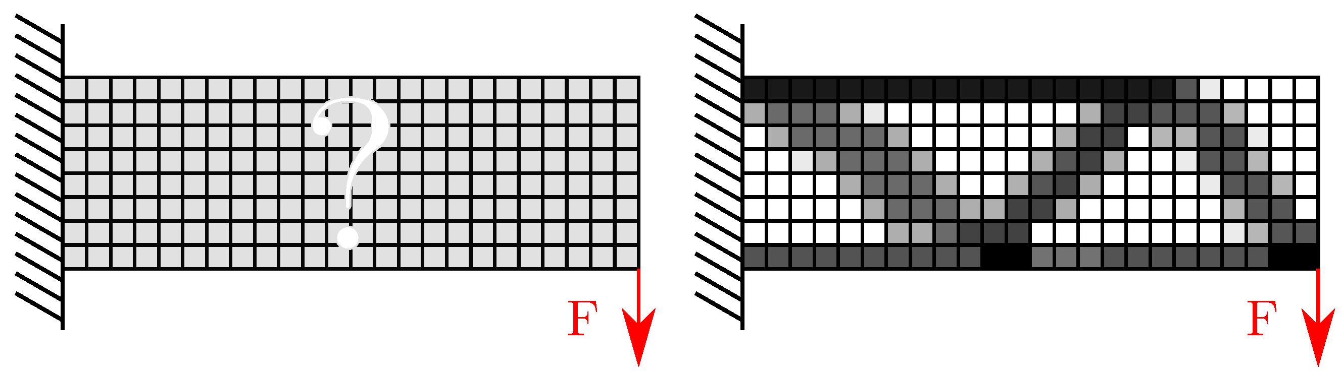
Topology optimization is a calculation of the distribution of materials within a structure without a known pre-defined shape. This distribution calculation yields a “black and white pattern” where black places indicate full material while white places represent voids (i.e., places where material can be removed). Because the distribution is solved over a general region, topology optimization allows us to acquire a unique, innovative, and effective structure. The principle of topology optimization is presented on the example of cantilever bending in Figure 1, where the initial geometry (given space) is depicted on the left and the optimal shape on the right. As apparent from Figure 1, topology optimization plays nowadays an important role in engineering practice. Usually, it allows the designer to reduce the weight of the part without losing too much of its previous properties such as stiffness, natural frequency, etc.
Issues associated with topology optimization are studied by many engineers and researchers. The Finite Elements Method (FEM) is the most widely used technique for the analysis of discretized continuum. Femlab [1], FreeFem++ [2,3] and ToPy [4] are rapidly growing engineering tools supporting topology optimization. The problem of topology optimization was described, e.g., by Bendsøe and Sigmund [5,6,7,8]. Many computer tools have been prepared, including tools in the MATLAB platform (MathWorks, Natick, MA, United States of America). Liu et al. [9] described a three-dimensional (3D) topology optimization using MATLAB scripts. They described the necessary steps of optimization and provided scripts for individual steps. Their scripts are freely available and can be modified in accordance with the authors’ instructions. It should be noted that although the scripts have great educational value, their practical usage is limited as they are applicable only for simple shapes and cannot work with imported meshes. The same can be said about the paper by Sigmund et al. [7] who investigated two-dimensional optimization and introduced sensitivity filtering. Master thesis by William Hunter [10] worked on 3D topology optimization. The author described in depth the theoretical background as well as its implementation in Python.
Even though topology optimization might seem novel, the first mention of structural topology optimization dates back to 1904 [11]. However, major progress has come only in the last 30 years due to the development of computers and the advancement of new technological processes (in particular, additive manufacturing). Hunar et al. [12] and Pagac et al. [13] illustrated the significance of topology optimization for designing a 3D printed part. Currently, however, topology optimization is perceived by most users as a “black box” producing always correct, i.e., optimal, shapes.
This is, however, largely not true and deeper understanding of the parameters and settings is needed to yield optimal results. A thorough introduction to the problem and a complex guideline for performing sensitivity analysis that would help researchers and engineers with determining correct settings is, however, not available in the current literature. For this reason, we decided to provide such a guideline in this paper.
Hence, the presented paper studies the effect of key formulations of the topology optimization problem on the design performance. In addition, it recommends the values of individual numerical parameters using a cantilever beam problem. Even though it is demonstrated on a simple example, this insight can be used for complex problems of engineering practice. For example, our group [14] described topology optimization of a transtibial bed stump using a custom MATLAB script. Performing sensitivity analysis of the key formulations is recommended for supporting the robustness of the computations in any new problem. Failure to perform so such an analysis may lead to the production of „false-optimal“ results. The individual steps of this study were performed in MATLAB as well as in ANSYS Workbench 2019 R3 (ANSYS, Inc., Canonsburg, United States of America, AWB), which helped with the evaluation of the results (assessment of the similarity in resulting values or shapes). The preliminary results of the work are presented in the Master’s thesis by Sotola [15].
2. Materials and Methods
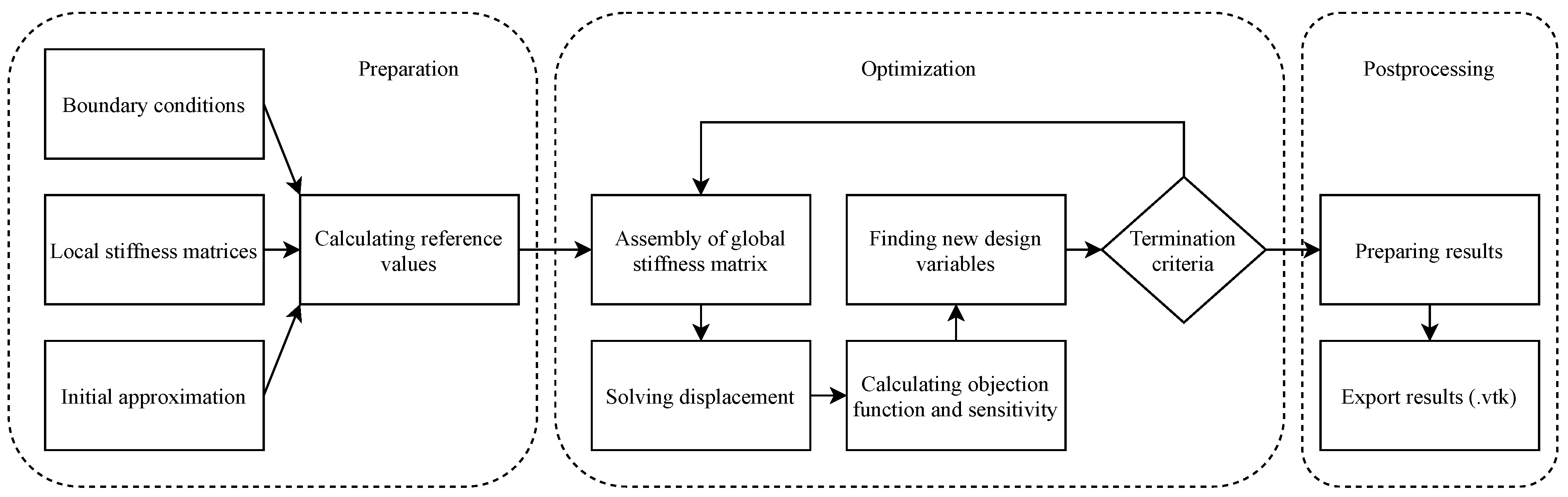
The procedure for calculating the optimal shape of the structure can be divided into three stages: (i.) Preparative stage (ii.) Optimization, and (iii.) Postprocessing, see Figure 2. MATLAB scripts were prepared for each of these stages to automatize the procedure.
The first step of the initiation of optimization lies in preparing the finite element analysis. In this step, the boundary conditions and local stiffness matrices of elements are set up. This paper does not describe this stage in depth because it has been already described in many books; for example, Hughes [16] describes the preparation of local and global stiffness matrices. Still, some advanced recommendations are presented in this paper. At this stage, the global stiffness matrix is also assembled and the reference values of the objective function are calculated. Before optimization, it is also necessary to prepare an initial approximation of volume, i.e., the structural elements are assigned a new material model containing individual design variables for each element. Elements are assigned new values of elasticity modulus, which affect the global stiffness matrix and leads to a new value of the objective function with each iteration.
Optimization itself follows, during which new values of design variables are determined. Subsequently, the terminating criterion is queried and if the process is not terminated based on the criterion being met or the maximal number of iterations exceeded, the process is repeated with new design variables.
In the last stage, the results are recalculated and prepared in the format, which can be viewed in the open-source software ParaView (Kitware, Inc., Clifton Park, NY, USA). This paper focuses on the first and second stages; we provide the results of the entire process but do not describe the postprocessing in detail.
2.1. Description of the Optimization Problem
As mentioned already, being able to describe the problem as a mathematical input is the key to the full understanding of topology optimization. Such understanding is needed for proper definition of the design variables, the objective function, and the constraint function (mostly inequality constraints). The most widely used method for solving multivariate optimization is called “Karush–Kuhn–Tucker conditions” [17] (also known as Kuhn–Tucker conditions or just KKT conditions).
2.1.1. The Optimization Problem
The objective of the optimization presented in this paper is to minimize compliance arising during volume reduction defined as volume fraction . The volume fraction is calculated as the ratio of the proposed volume and the original volume. The volume fraction ranges from 0% to 100%.
Several methods can be used for solving the problem of minimization of compliance. For example, the homogenization method [18,19] uses microperforated composites as a base material for shape optimization. Since the number of holes within the domain is not limited, it can be seen as a method of topology optimization. In another approach, the phase-field method, the domain consists of two “phases”, the “void” and the fictional “liquid” which interacts with loads [20,21]. One of the newer methods (meaning newly implemented in commercial software) is the Level-set method. Optimization in this method is solved “above” the fixed domain with a fictional velocity [22].
The density-based method is the last of the methods commonly used for solving the topology problem. This method can be viewed as mature and is easy to implement. In this paper, we focused on this method, which uses a continuous design variable ranging from 0% to 100%, see Figure 1. In the literature, the design variable is usually referred to as the density; note, however, that this “density” of the element has no clear physical meaning. In 2D space, the density can be pictured as a variable thickness of sheet metal but in 3D space, it is not easy to assign a tangible meaning to this term. The Solid Isotropic Material with Penalty (SIMP) model is a popular interpolation scheme for definition of material that would be subsequently used in the density-based method. In this model, the elasticity modulus is in a power law relation with the design variable and can be described using the following equation.
where is the elastic modulus of the base material, p is the penalization and is the “modified” filtered design variable. The reasons for the “modification” are described in the following Section 2.1.2 and Section 2.1.6.
After preparation of the material model, the objective function of minimizing compliance is defined as
where c is the deformation energy, is the force vector and is the displacement. One could argue that the deformation energy of the linear material should be divided by two; however, as it is only a scalar variable, it will not affect the optimization itself. The constraint Equation (or, rather, inequality in this case) is defined as
where is the vector containing the volume of each element. Displacement is solved from the equilibrium equation
where is the global stiffness matrix. Assembly of stiffness matrices is described in Section 2.1.4. The design variable is defined as
Equation (2) can be written in a simpler form after applying SIMP
where is the vector of element displacement, [k0] is the stiffness matrix with unit elastic modulus and n is the number of elements. Penalization is introduced in Section 2.1.3.
One can notice that the problem is defined as minimizing the deformation energy, which leads to the higher stiffness of the structure. Using the KKT conditions, the Lagrange multipliers convert the constrained problem to the equivalent unconstrained problem [17,23]. The first step is assembling the Lagrange function
where is the objective function, is the constraint function and the Lagrange multiplier. It is necessary to solve the derivation of the Lagrange function with respect to the design variables because it is necessary to find a stationary point; at that point, the derivation is equal to 0
The following equation is known as the complementary slackness condition, determining whether the constraint function is active or passive
The next condition is that the Lagrange multiplier is not negative
The last condition is the derivation of the Lagrange function with respect to Lagrange multipliers. In simple terms, it determines whether or not the particular point is the KKT point, i.e., the optimum (there are fundamental theorems proving that the solution is automatically optimal, see more in [17]). This condition is not important for solving the problem, it is important for results evaluation. Rearranging the equation and adding the variable leads to the equation
It is obvious that the optimum of the element is met if . Preparing the first derivation of the objective function determined by Equation (2) with respect to the design variables can be tricky as at the first sight, there is no evident “influence” of the design variables. It can be solved numerically but this would require a calculation of the displacement for every individual possible design variable. However, it is possible to calculate derivation using the adjoint method [5], i.e., to add the equilibrium equation into the objective function
where is a vector of non-zero variables (also unknown for now). Adding the equilibrium equation does not change the objective function because it is equal to zero. Similarly, the vector does not change the function. Let us assume that the exterior forces are not independent on the design variables. Then, the first-order derivation of the objective function is
Rearranging the previous Equation (13) leads to factoring out the derivation of the displacement
To get rid of the derivation of displacement, it is critical that the term in brackets (adjoint equation) is equal to zero. This means that our added unknown variable has to be equal to
It is apparent that the vector is already solved. The final form of the derivation of the objective function (with added SIMP model) is
The first order derivation of the constraint function is defined asIt should be noted that in the literature (for example, [8]), it is possible to find another equation describing the constraint function and its derivation
It should be noted that in the literature (for example, [8]), it is possible to find another equation describing the constraint function and its derivation
That form of the equation usually depends on the solver and its settings. For example, “MMA-based” solvers prefer the constraint function defined by Equations (18).
2.1.2. Material Model
In this paper, the density-based method used the Solid Isotropic Material with Penalty (SIMP) material model, which is a power-law relation of the design variables. The SIMP material model is used in solvers such as ANSYS (ANSYS, Inc., Canonsburg, PA, USA), MSC Nastran (MSC Software, Irvine, CA, USA), etc. The elastic modulus of the element is defined as
where is the elastic modulus of the base material, p is the penalization and is the “unmodified” design variable. This definition looks very similar to Equation (1); however, here, we use unfiltered designed variable to give a clearer picture of the need for filtering (see below).
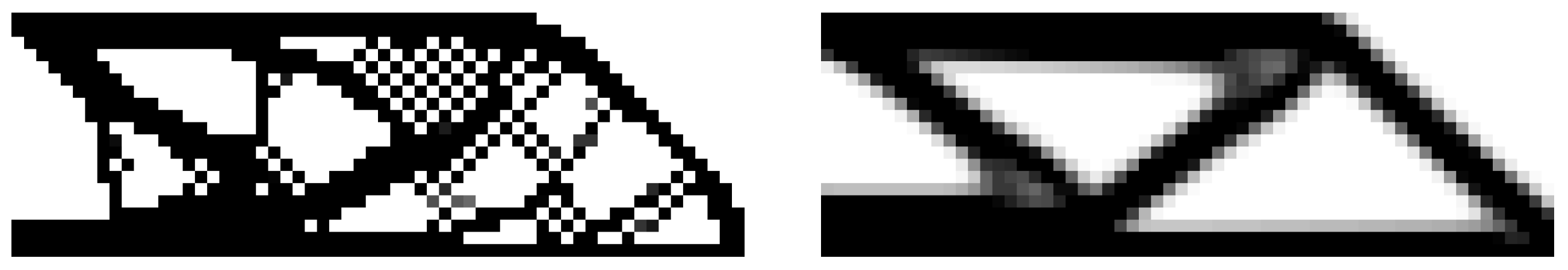
During topology optimization, many problems can occur. For example, the so-called checkerboard pattern problem [24,25,26] is very common. This title describes the distribution of the structural elements in a checkerboard-like arrangement in certain areas of the part. Figure 3 shows the checkerboard patterns on the cantilever beam.
In our case, i.e., when discussing the problem of minimizing compliance, the computation may consider such a solution to be ideal as the checkerboard pattern creates artificial regions with higher stiffness. However, as obvious from Figure 3, this is not true and, moreover, the part cannot be manufactured. Another common problem is the insufficient number of connected nodes (four or more nodes are needed for the hexahedral element), which causes the formation of possible joints in the structure and, again, makes it impossible to manufacture.
The mesh-dependency of optimization results is a crucial problem [5,26]. As the name suggests, this problem results from the used discretization and its refinement. In context of structure stiffness, the reason is quite simple—increasing the number holes in the structure without changing its volume leads to increase of stiffness. Finer meshes facilitate this operation—they allow us to create a higher numbers of holes and, therefore, are capable of providing different (superior) results than coarser meshes. On the other hand, finer meshes might result in more complex structures that are difficult to manufacture.
The last important problem of topology optimization is the non-uniqueness of solutions, which makes results evaluation trickier [27]. Generally, the problem of optimization can have a single solution or up to an infinite number of solutions depending on whether the problem is convex or not.
One of the ways of solving the above-mentioned problems is to use a suitable filter(s). This solution has not been mathematically confirmed, but many numerical experiments suggest that the results could be considered optimal [7]. The description of each of the filters used in our study is presented in Section 2.1.6.
To prevent numerical difficulties, the modulus of void (passive) elements is introduced into the material model. This modification helps to reduce the risk of having a singular stiffness matrix. The final equation of the material model is
where is the elasticity modulus of passive elements and is the filtered design variable (density).
2.1.3. Penalization
The numerical scheme should lead to a black & white design (or 1-0 design with white to be removed). One of the possible approaches is to ignore the physical importance of elements with intermediate density (grey areas) and consider them “black”, leading to their preservation. However, the physical relevance is discussed a lot since many interpolation methods can remove further parts of the grey regions. If the optimization is prematurely terminated, the stiffness (compliance) of the grey areas plays an important role in the evaluation of results. This issue is discussed by Bendsøe [5,6]. As mentioned above, the SIMP material model is suitable for FEM optimization as it assigns elasticity to each element. However, it can be used as the material model only if the penalization meets the following criteria
where is the Poisson’s ratio. This means that different values of penalization must be calculated for each Poisson’s ratio. The resulting values of the penalization for volume elements with the following Poisson’s ratio are
In this paper, the base material has a Poisson ratio of ; therefore, the penalization was chosen for the following topology optimization.
2.1.4. Finite Element Method
From our experience, it is recommended for MATLAB implementation that the stiffness matrices is prepared with unit elastic modulus and saved in memory. The stiffness matrix of the solid element is volume integrated using the stress–strain matrix of the material with the unit elasticity modulus
where is the strain–displacement matrix [28]. The integral is usually solved numerically. Before the assembly of the global stiffness matrix, every local stiffness matrix is multiplied by the corresponding elasticity modulus (i.e., the modulus of the SIMP material model).
The MATLAB implementation of calculating the stiffness matrix of linear elements is presented by Bhatti [29,30]. With some effort, the procedures were modified to the calculation of quadratic elements. The procedures use full integration of the individual elements using Gauss points (2 × 2 × 2 scheme for linear elements, 3 × 3 × 3 for quadratic elements).
For testing purposes, meshes were prepared using the AWB software [31]. They were constructed either of tetrahedral (TET) or hexahedral (HEX) elements (i.e., no result with mixed mesh was evaluated in this paper). The calculation of the stiffness matrices of linear elements is fast thanks to the low number of degrees of freedom (DOF); in effect, solving a single load case was swift when using this approach; however, it comes with a disadvantage in the form of locking as linear elements with full integration have a tendency to shear and volume locking [28]. There are numerous ways of fixing this problem; nonetheless, in this paper, the shear locking effects are “neglected” during the optimization but are mentioned in results. Meshes are separated into three groups: coarse, normal, and fine meshes according to the size (length) of individual elements.
2.1.5. The Optimality Criterion Algorithm
The design variable of the elements was updated using an algorithm called the Optimality criterion (OC) [5,32]. The name indirectly refers to the used method, i.e., KKT conditions. The algorithm is also implemented in the AWB software. To find the material distribution of the structure, a fixed updating scheme is proposed as
where is constructed using Equation (11). As already mentioned above, the optimum of the element is found if . In other words, the design variable increases if and decreases if . Changing the move limit m and tuning parameter can lead to a lower number of iterations. Bendsøe [5] recommended values of and . New values of design variables depend on the Lagrange multiplier, which has to be solved in the inner loop to ensure that the constraint function is satisfied. This leads to a reduction of the multivariate problem to one-dimensional (1D) optimization, which can be solved by various methods, such as the bisection method, golden section search, or methods using derivation (such as the Newton–Raphson method or secant method) [17,23]. In this work, the bisection method obtained from the paper by Liu [9] was used as the 1D optimization method.
A detailed description of the Optimality criterion method is presented in the dissertation thesis by Munro [32] and the Master’s thesis by Hunter [4]. These theses describe the relationships between the Optimality criterion and Sequential approximate optimization (SAO). The SAO method can be solved using the duality principle. The purpose of this method is to find an equivalent subproblem (dual problem) that is easier to solve than the primary problem. The method is used for preparing a scheme (similar to the OC fixed scheme) with only one constraint function, which can be subsequently solved. The primary problem (in this case, minimizing compliance) is then reduced to maximizing the Lagrange multiplier.
2.1.6. Filtering Methods
Density filtering is one of the methods of solving the above-mentioned problems (such as the checkerboard pattern). A common parameter of the filters, weight factor , is defined as
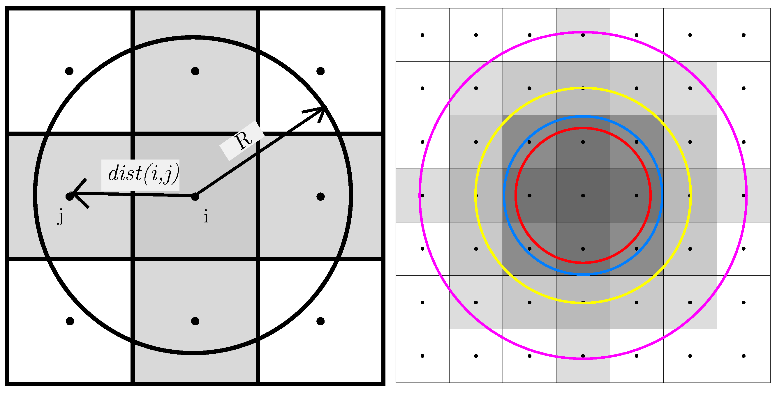
where R is the radius of the filter, is the operator calculating the distance between the center of an element i and the center of an element j. This type of weight factor is called linear. If the distance between elements is greater than the radius, the weight factor is equal to zero; if the distance is equal to zero, the weight factor is equal to the size of the radius. In Figure 4, 2D examples are presented; in 2D, the radius defines a circular neighborhood. In a 3D problem, the radius forms a sphere.
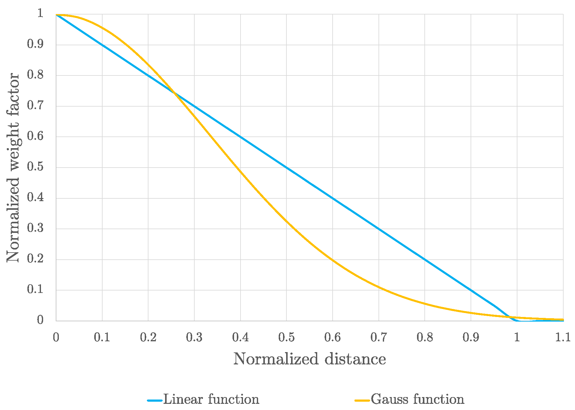
An alternative approach is to use the normal distribution (Gauss function) [33,34]. Compared to the linear function, the Gauss function is smoother but in reality, there might not be a real benefit in using this alternative [8]. The weight factor is defined as
In Figure 5, both functions are displayed. Due to the different characters of values of the weight factor, the linear function had to be normalized by the radius to have values ranging from 0 to 1, the same as the Gauss function. Furthermore, the distance was normalized to the radius (i.e., divided by the radius to ensure independence on it).
Preparing a matrix of weight factors can be challenging if the mesh is imported (if the mesh is not imported but created by additional scripts, the weight factor can be calculated during the mesh preparation). The following should be pointed out: Firstly, the preparation should use a function for creating sparse matrices because the matrix of weight factors is mainly sparse. Secondly, if the distance between the i-th and j-th element is constant, there is no need to create a “full” matrix but only the upper triangle of the matrix . Non-diagonal components of the matrix are multiplied by 2. The following equation uses “symmetry” for composing the full matrix
where T is the operator of the transpose. Lastly, with the growing amount of elements, the process of preparation is becoming more time-consuming even though calculating only “half” of the matrix. This basic approach is, up to 10 k elements, fast. However, the time of solution is growing exponentially for meshes with over 10k elements. In such cases, it is recommended to invest time into finding an appropriate method for speeding up the preparation. This could be done by dividing the mesh into mutually overlapping subzones with less than 10 k elements to ensure fast calculation. These subzones should be solved individually using the parallel toolbox (package). Using this approach, it should be possible to prepare the weight factors of complex meshes in a reasonable time.
Three filters are analyzed in this paper: (i) Density filter, (ii) Sensitivity filter, and (iii) Greyscale filter (G). The Density filter (D) and Sensitivity filter (S) use weight factors while the greyscale filter is an addition to the OC scheme.
Density Filter
The fundamental function of density filtering is
where is the filtered design variable (density) of the i-th element, is the weight factor and n is the number of elements [35,36,37]. Every equation containing the design variables has to be adjusted to allow filtering (including partial derivations)
In this case, the design variable of the element is averaged over its neighborhood. It ensures the smoothing of stiffness. The filtered density is applied during the construction of the global stiffness matrix before solving the static structural analysis. Generally, the density tends to have a value of 0 or 1 (which could be ideal), but after applying the filter, regions of intermediate (grey density) design variable appear, which are then penalized by the SIMP model. Deformation energy is also averaged and shared with the neighborhood of elements.
Sensitivity Filter
This filter is based on filtering of the sensitivity (i.e., of the first partial derivation of Lagrange function). Experience has proven that filtering sensitivity ensures mesh independence of results and is time-effective [7]. It is also easy to implement and does not increase the complexity of the problem. The filter is purely heuristic but has been proven to yield similar results as the gradient constraint method [5]. The fundamental equation of this filter is
Grayscale Filter
The last filter is an addition to the previous filters called the Grayscale filter [38]. Applying this filter should reduce the grey areas. The objective of the filter is also to penalize the volume constraint in the OC algorithm. The parameter q is implemented in the OC scheme and its value can be constant or gradually increasing by multiplication (in our case, coefficient q was multiplied by 1.01 each iteration). The amended OC scheme is described as
This filter is activated after 15 iterations of optimization. Usually, it is limited by the maximum value of the coefficient q (in this paper, the maximum was set to 5). If the q coefficient maximum was set to 1, the filter would be deactivated. The idea of the filter is to underestimate the intermediate density leading to a zero value (void density). Underestimation occurs also in the inner iteration. This leads to fewer iterations needed for finding solutions.
2.1.7. Displacement Solver and Termination Criteria
To solve the displacement Equation (4), it is possible to use the direct solver present in MATLAB. However, if the number of degrees of freedom is high (above sixty thousand), the pursuit to provide an accurate result is too ambitious. In such cases, therefore, it is appropriate to switch to the iteration solver. MATLAB includes a solver using the conjugate gradient method with preconditioning [39]. It is recommended to use the simplest preconditioning matrix, the diagonal (Jacobi) preconditioner. The reason is that to ensure the best possible solving stability, assembly of the preconditioner is needed in every iteration and, hence, the simpler is the preconditioner, the faster is the solution. Use of a different (more complex) preconditioner, such as Incomplete Cholesky factorization (with various settings),could reduce the number of iterations but the computing time would be the same or higher due to a slow preconditioner assembly (we tested these in the preliminary stage but the detailed results are not presented here). An alternative approach would be to prepare a “universal” preconditioner from the reference matrix only once and to use in every iteration [40]. In the presented study, however, we used the first approach with assembling the diagonal preconditioner each iteration.
It is important to determine the termination criteria. The maximal number of iterations is the first common criterion. Usually, the value ranges between 200 and 500. It should be noted that a complex task (such as a complex geometry or complex loads) requires more iterations but from our experience, 100 iterations are enough for a simple task. The second criterion is defined as the tolerance of sufficient optimization at which the calculation is terminated. There are two possible options.
The first option is to calculate the change in the values of design variables between the current and previous iteration [7]. This change is compared with the chosen tolerance value and once the change in the design variables is below the tolerance value, the calculation is terminated. Thus, if the tolerance is set to a low value, the number of iterations will increase. This is defined as
where are the design variables of the current iteration, are the design variables of the previous iteration and is the tolerance value.
The other option is to calculate the ratio of the change of the objective function to the current objective function value. It is assumed that the changes of the objective function near the stationary point are minimal. Compared to the first option, the number of iterations is lower (it may be reduced by as much as half). This option is defined as
where is the value of the objective function in the i-th iteration, is the value of the objective function of the previous iteration (i−1), and is the tolerance value. This method, however, comes with a risk of premature termination; for this reason, the first option of terminating criterion was used.
2.2. Key Formulations
It is apparent from the previous sections that the optimization comes with many formulations and parameters. Each parameter can be changed, which might reduce the number of iterations, improve the values of objective functions or of the desired volume fraction; on the other hand, the changes may also lead to solver instability, premature termination, or ineffective shape of the part. In this paper, five key formulations are analyzed and evaluated:
Formulation of the filter radius mentioned in Section 2.1.6 is important because the radius defines the element’s neighborhood. If the defined range is too small, the energy is distributed only to a few elements. However, if the neighborhood is too large, the energy is scattered to a point where it is difficult to evaluate the optimum.
Formulation of the filter type was already mentioned in Section 2.1.6 but the theory does not provide an answer to the question of which filter should perform best.
Formulation of the penalization was also mentioned in Section 2.1.3; the theory, however, is able to provide only the lower boundary, not the upper one.
Formulation of the element approximation mentioned in Section 2.1.4 is a necessary step in the initiation of optimization. The element approximations greatly affect the accuracy of the solved displacement and the value of the objective function.
The formulation of the type of the weight factor mentioned in Section 2.1.6 is defined by two functions. However, theory does not provide enough evidence to decide, which function offers the better performance.
These key formulations were tested on several numerical examples including planar and spatial problems (see Figure 6) but to ensure the clarity of this paper, only one example is presented.
2.3. Description of Numerical Test
The sensitivity analysis was performed using a numerical test-cantilever beam. It is a standard problem of mechanics, well-known to every designer. As the optimal shape can be found intuitively, results evaluation is easier.
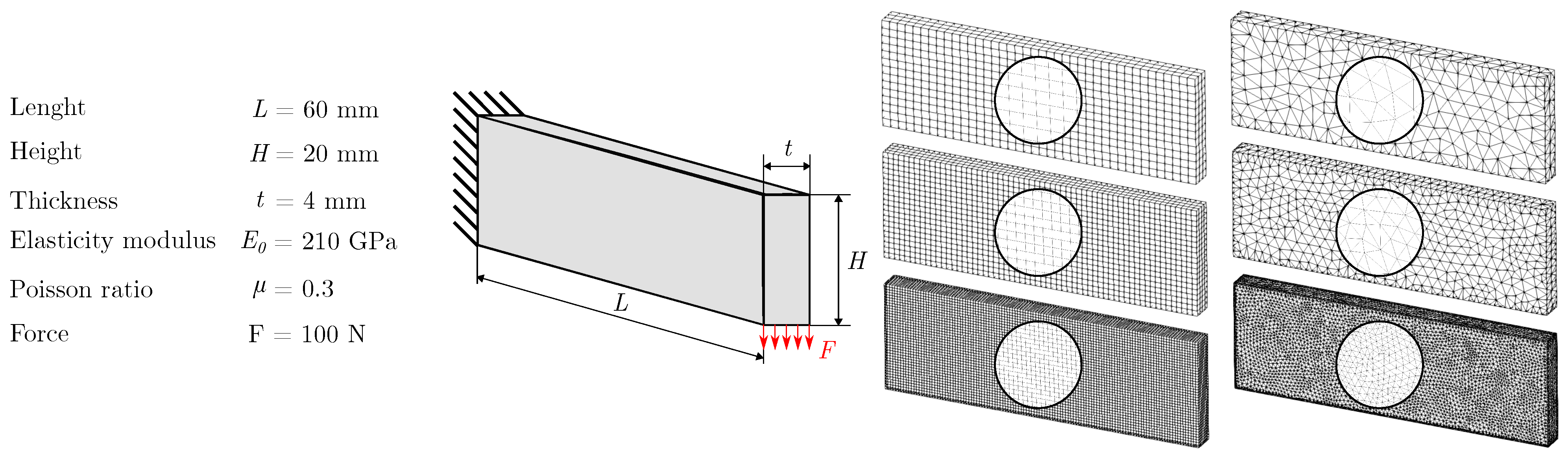
The boundary conditions were simple. The beam was fixed on one end and the force acted on the other end’s edge (bottom edge). The beam had a rectangular cross-section and was made of steel. It was assumed that the forces caused only a small displacement and the original material model was linear isotropic. All finite element meshes were made of solid elements, see Table 1. The authors used linear HEX elements and linear TET elements. In addition, quadratic HEX and TET elements have been calculated and results (mesh statistics) presented in Section 3.4. The geometry and discretization are shown in Figure 7. The figure also contains material and force parameters. The objective of optimization was to minimize the compliance (i.e., to maximize stiffness). In our paper, the constraint was defined as the volume fraction of 30%.
3. Results
Optimization using MATLAB software was performed on multiple meshes. The maximal number of iterations was set to 200. The maximal change of the design variable (i.e., density) was chosen as the terminating criterion. The tolerance was set to 0.01. The cut-off limit of the design variable for element deactivation (white in the Figures) was 0.01 unless stated otherwise. The penalty was set to a constant value of unless stated otherwise. Unless stated otherwise, the Density filter was used throughout the paper. In tables, two variants of the objective function are shown. The non-normed value indicates the deformation energy. The normed value is the objective function divided by the reference value of the initial objective function (i.e., the objective function describing the original structure before optimization). In other words, the normed value shows how many times the resulting structure is more compliant than the original reference. The normed value in the linear static analysis should be the same (or, at least, similar) regardless of the applied force. Data and shapes presented in this chapter were prepared in Ansys Workbench (AWB).
3.1. Formulation of Filter Radius
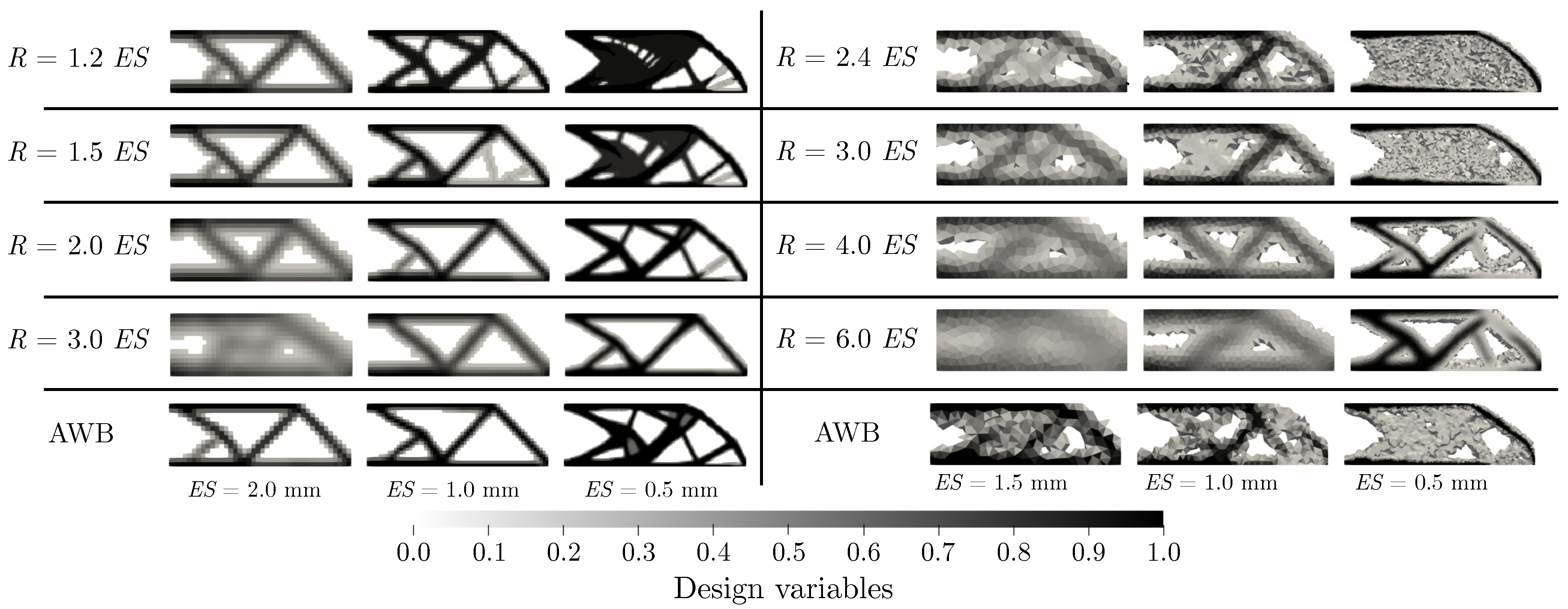
The radius of the filter is an important parameter since it defines the element’s neighborhood. In this case, the radius is dependent on the element size (). For hexahedral elements, multipliers were set to 1.2 , 1.5 , 2.0 , and 3.0 , respectively. For clarification, Figure 4 displays the mentioned radiuses. For tetrahedral elements, multipliers were twice as high (i.e., 2.4 , 3.0 , 4.0 and 6.0 ) to prevent possible inactivation of filters.
Results for the hexahedral and tetrahedral meshes are shown in Figure 8, which is displayed in the dominant (planar) view.
From Table 2, it was apparent that the radius heavily affected the distortion of design variables over the design region. This means if the radius was increased, the value of the objective function (both deformation energy and normed value) also increased. Besides, the volume fraction increased due to the distortion. A fine mesh with small radii yielded a great stiffness-volume ratio, the optimized structure was approximately 2.5 times more compliant than the original structure but the volume reduction was as high as 53%.
A few notes: Radius should never be smaller than . A radius such as 1.2 greatly limited the capability of filters. In the case of uniform mesh, the radius should be appropriately chosen from the range between and . In the case of the non-uniform (tetrahedral) mesh, the radius should be within the range of to . Radii exceeding the upper value of the mentioned ranges make the structure more compliant. In the case of a coarser TET mesh, the radius caused an over two-fold increase in the deformation energy than radius . Besides, the shapes of the coarser meshes with larger radii were not acceptable due to the high representation of “grey” areas (see Figure 8).
3.2. Formulation of Filter Type
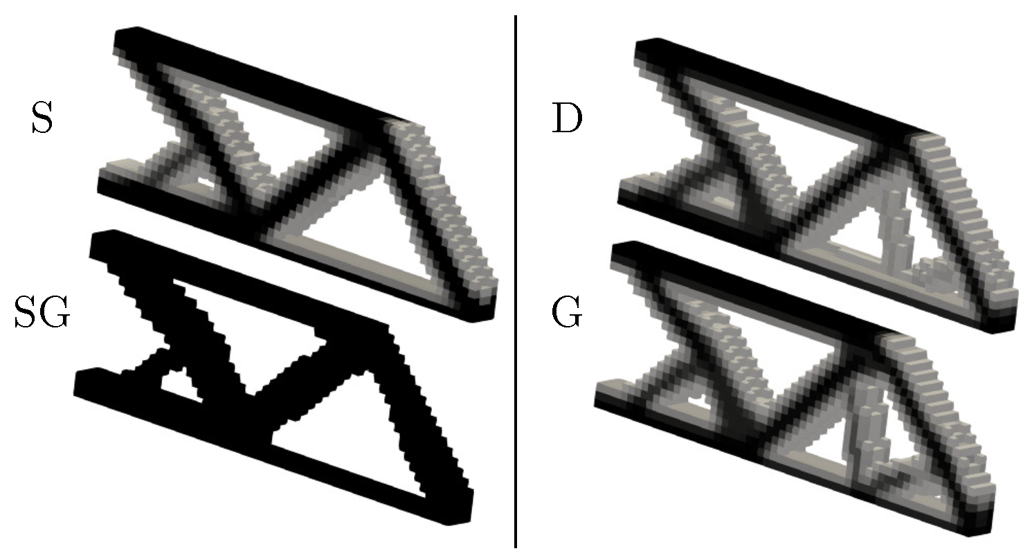
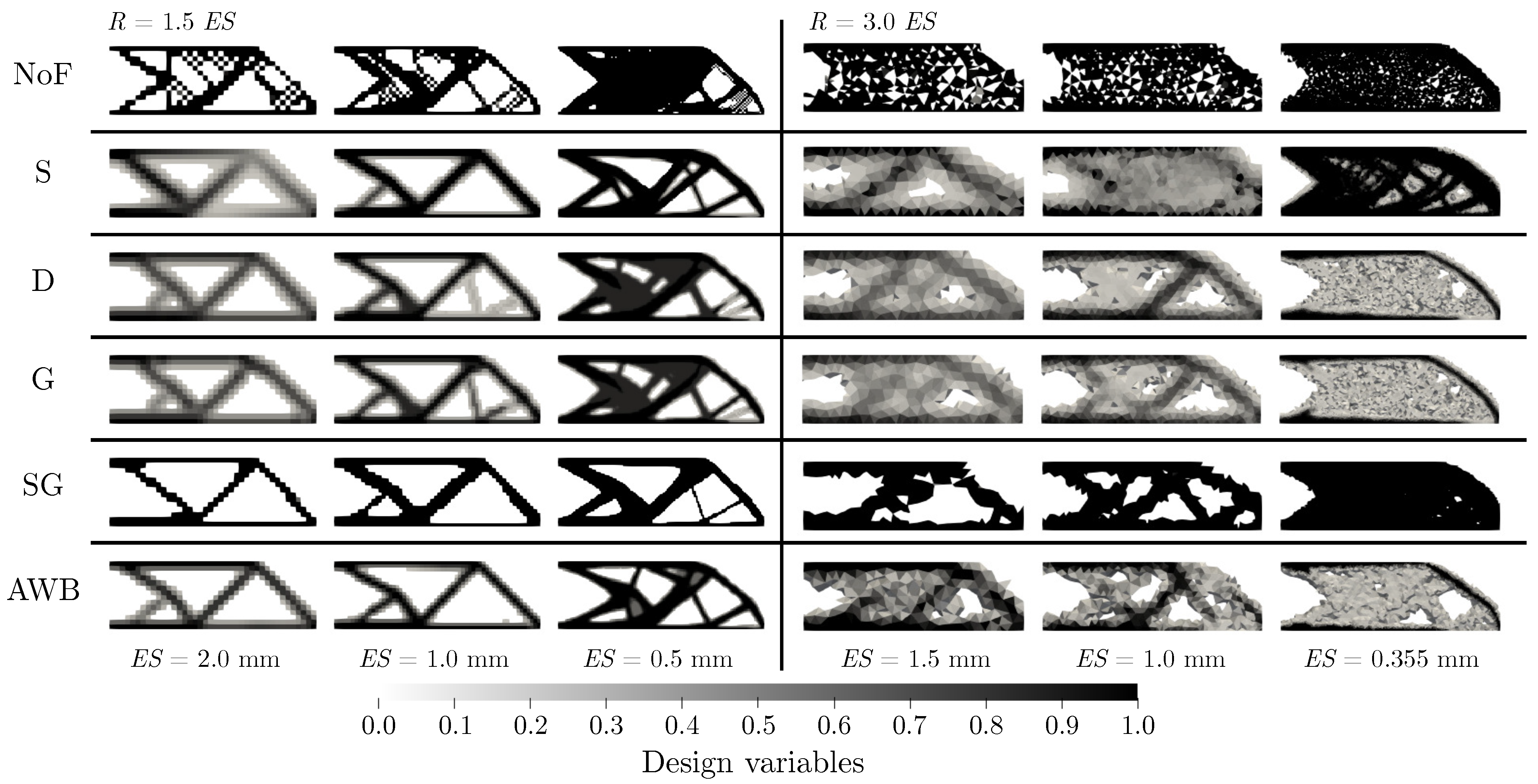
The importance of filters was already mentioned in the previous section. The following effects were evaluated: the number of iterations, objective function, and volume fraction. This particular aim of our study was to find the appropriate filter leading to a 0–1 design (and low objective function). Five variants were calculated: No filter (NoF), Density filter (D), Sensitivity filter (S), Grayscale filter with Density filter (G), and Grayscale filter with sensitivity filter (SG). Figure 9 shows each filter.
At the first look, it should be apparent that the SG combination leads in this case to a purely 0-1 design (with the required volume fraction).
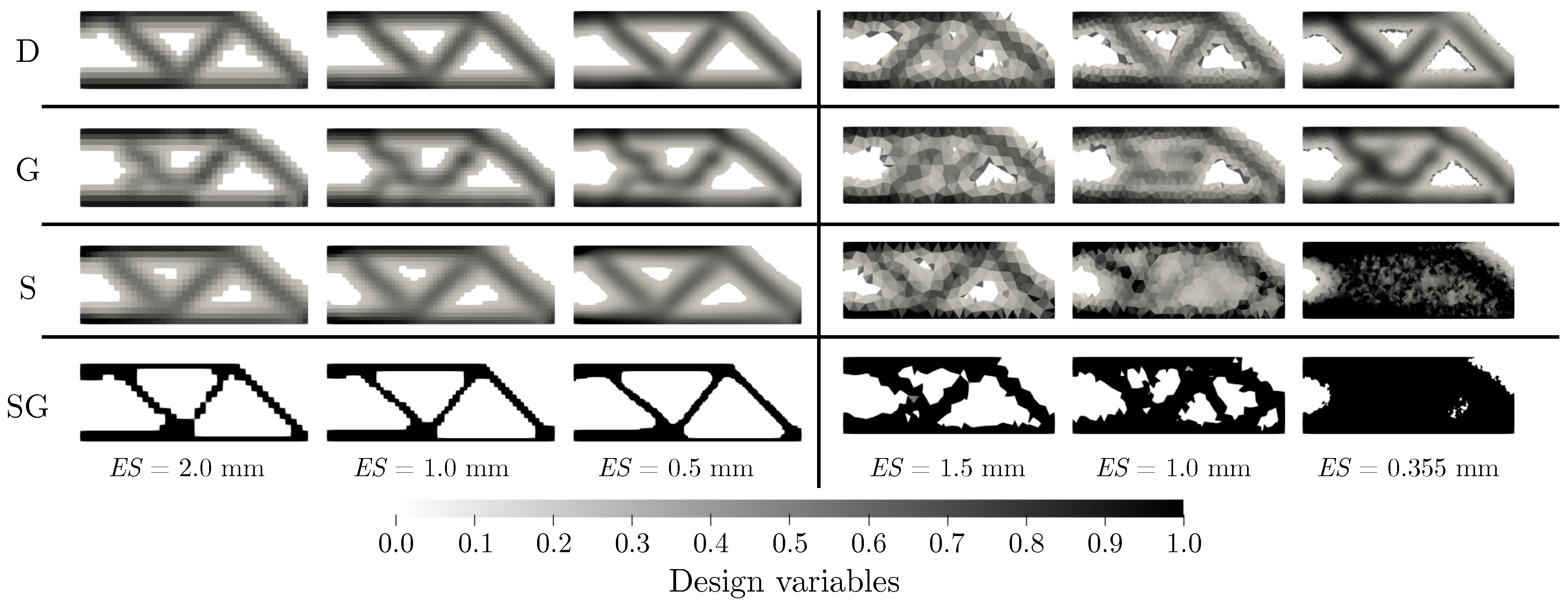
Two variants of the radius were selected: In the first variant, the radius was considered to depend on the element size, namely, it was defined as 1.5 . Results of this approach are displayed in Figure 10 and Table 3. The way of how the filters acted when the radius was not constant over different meshes should be noted.
In the second variant, the radius was not considered to be dependent on the element size and was assigned a constant value of mm. This radius was defined as a 1.5 multiple of the element size from the coarse tetrahedral mesh. Results displayed in Figure 11 and Table 4 demonstrate the independence of the results on the mesh (results have a similar shape and value of the objective function). In this variant, TET meshes performed poorly, especially in combination with the Sensitivity filter, which acted unpredictably at best. A coarser TET mesh could result in an acceptable shape (i.e., a shape similar to that derived using the HEX mesh) but finer TET meshes did not lead to volume reduction, but rather to its increase. In addition, the combination of TET mesh with Sensitivity filter often resulted in premature termination of the computation.
It should be noted that unwanted effects, such as shear locking, can occur while solving the static structural analysis and cause an increase in the relative error of the objective function. In case of the radius of mm, the deformation energy of the Density filter was slightly higher for HEX elements than for TET elements. Hence, relative errors were small enough to justify acceptation of the results.
Our results indicate that all filters discussed in this paper are suitable for use with a uniform mesh. The recommended filter combines the Density or Sensitivity filter with the Greyscale filter to ensure a low number of iterations. In the case of a fine mesh, the Density filter without the Greyscale filter reached a maximal number of iterations while with the Greyscale filter, only 34 iterations were needed. The deformation energies of both results were similar. In the case of a non-uniform mesh, only the Density and Greyscale filters can be used effectively.
One could argue that the combination of the Sensitivity and Greyscale filters got us a perfect black and white design with the required volume fraction (volume reduction of 70%) while increasing the compliance of the structure only approximately 2.1 times; however, the shape was likely to be prone to buckling since compared to other results, the parts were thin.
3.3. Formulation of Penalization
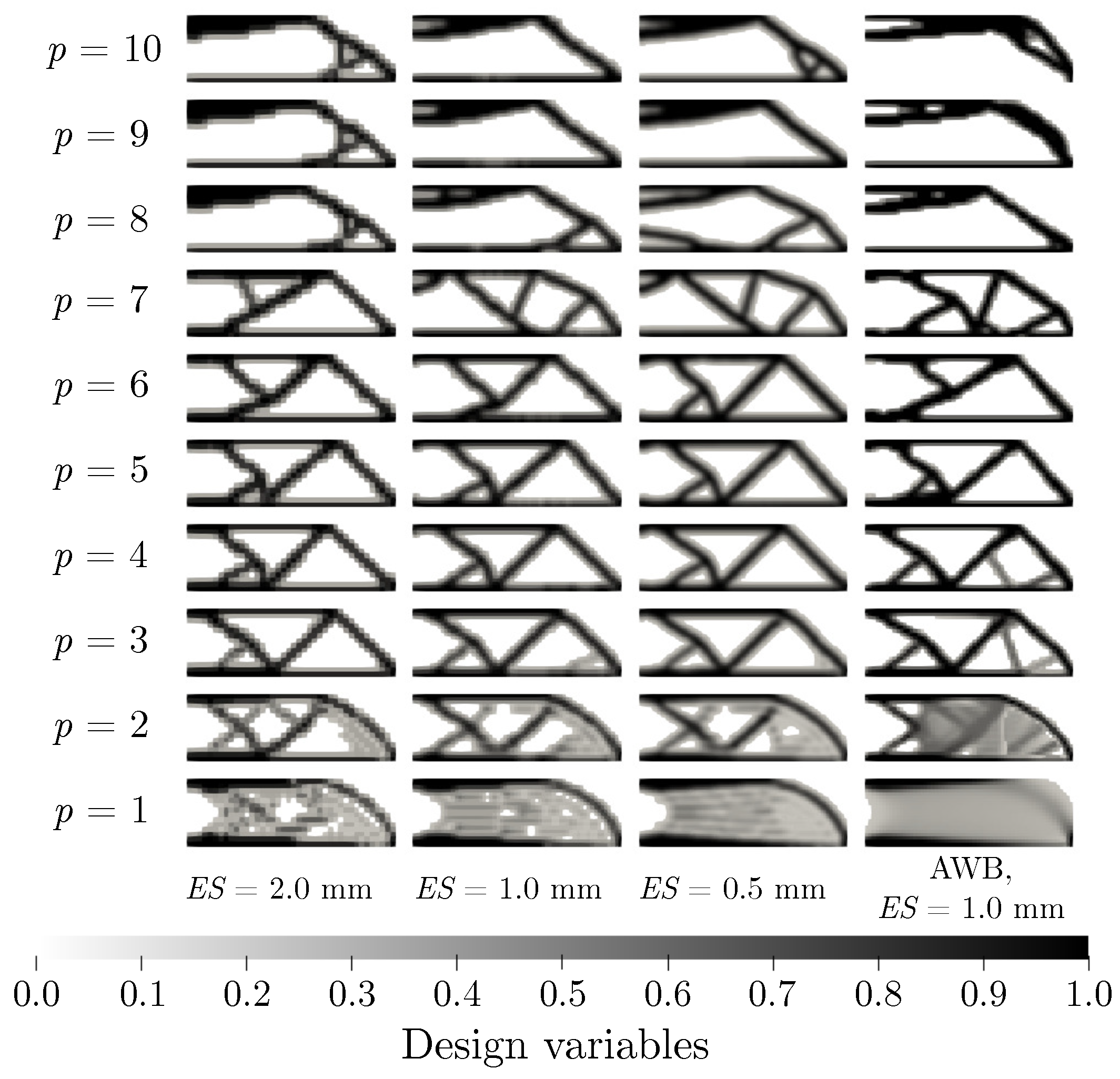
Penalization is the parameter of the SIMP material model. Its correct choice is crucial as incorrect penalization would invalidate the model. For the Poisson ratio of , it is recommended to use the penalization of p = 3 and higher as mentioned above.
Figure 12 demonstrates that the penalizations and should not be used since the shapes are not fully optimized (due to the premature termination of optimization). Literature, however, does not set the upper limit of this inequality. The values of deformation energy grew more or less predictably up to a penalization value of , see the values in Table 5. With high penalization values, such as , it was, nevertheless, clear that the results were becoming mesh-dependent. This could be caused by the convergence of the solution to a local minimum rather than a global minimum.
One could choose the continuation method with a gradual increase in the penalization value. This approach should help in acquisition of a reasonable solution. It should be, however, mentioned that the continuation method might not be capable of yielding a true “black and white” design, as reported by Stolpe and Svanberg [41]. This paper does not fully study this strategy; the risks are that a too fast increase of the penalization could lead to numerical difficulties that only increase the number of iterations.
3.4. Formulation of Element Approximation
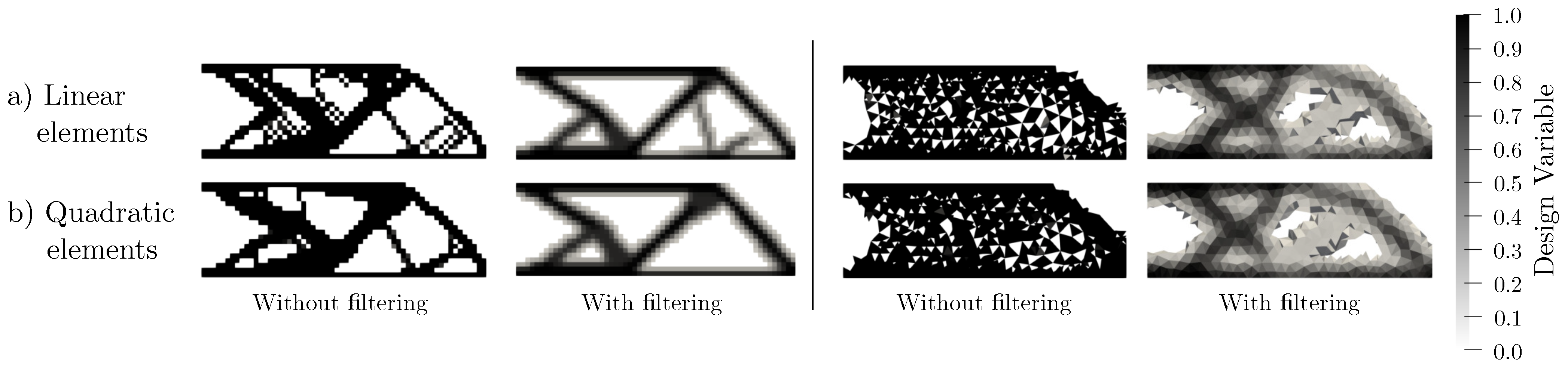
During the mesh preparation, it is necessary to choose an element approximation (usually linear or quadratic displacement approximation). Literature suggests that problems such as the checkerboard patterns should be less common with quadratic elements [26]. The advantage is that quadratic elements are less stiff than linear ones. However, the need to solve a larger number of unknowns (DOF) is a considerable disadvantage of this approach. Table 6 lists the mesh statistics.
In our case, the optimization settings were slightly altered. Only the Density filter with a radius of for HEX elements and for TET. Element size of mm was used. The maximal number of iterations was set to 100.
Figure 13 shows that the previous statement about the checkerboard pattern being less common with quadratic elements is only partially true. In the case of quadratic HEX elements, a checkerboard pattern was still present in the front part of the structure (although less than when linear elements were used). In the case of TET elements, not even higher order approximations did reduce the checkerboard pattern. Hence, filtering is highly recommended regardless of whether quadratic or linear elements are used. Table 7 obviates that the linear elements are stiffer, i.e., that they provide lower values of the objective function. However, the time needed to solve the problem with quadratic elements is up to thirty times longer than with linear elements.
3.5. Formulation of Type of Weight Factor
In the theoretical part, two types of weight factors are mentioned—one characterized by a linear function, the other by the Gauss function. Nevertheless, according to the literature, there is no evidence that the Gauss function offers any advantages over the linear one [8].
In the investigation of this formulation, only two meshes were tested. Both meshes used linear elements with element sizes of mm and mm. Two radii were chosen as and , respectively. The maximal number of iterations was 100.
The values of the objective function and volume fraction detailed in Table 8, as well as results shown in Figure 14, indicate a significant resemblance between values acquired using Gaussian and linear weight factors. In the case of a normal mesh ( mm), setting the radius of the linear function to provided similar results as in the case of the Gauss function with a radius of (see the highlighted values in Table 8). In the fine mesh ( mm), the similarities were more pronounced than in the normal mesh. This means that the Gauss function does not offer any significant advantage over the linear function as their results are very similar and shapes similar to those produced by the Gauss function can be obtained by simply changing the radius in the linear function/solution. As the preparation of mathematical apparatus is simpler with linear function, we decided to prefer linear solution over the one with the Gauss function.
4. Discussion
To fully understand optimization, one should possess advanced experience in math (namely, calculus and finite element method) and computer science (for example, scripting for iteration solvers). One should also be capable of preparing a correct mathematical formulation of the problem, i.e., of determining the objective function of the problem, constraints, and design variables, and of finding equivalent problems, potentially offering an easier solution than the original one.
Five key formulations were analyzed in this paper. The results make it clear that each formulation affects the resulting shape, number of iterations, volume of the part, etc.
The formulation of the filter radius is crucial for determining the element neighborhood. Choosing too small radius might lead to the deactivation of the filter. Choosing a too large radius leads to dissipation of energy in large areas, resulting in too much “grey”. Choosing the filter itself can be difficult since the theory does not provide enough knowledge from the application point of view. The SIMP model was used as a simple material model in this study. The penalty value is a key parameter of this model. However, the theory provides only the bottom boundary but does not inform about the upper one. Failure to limit the upper boundary could lead to invalid results that would be highly mesh-dependent. The maximum reasonable penalty value for the steel cantilever in our study was .
The theory also recommends a quadratic approximation of the displacement of the elements. However, it does not provide clear reasons behind this recommendation. Choosing the right approximation might lead to a faster calculation. Lastly, neither the theory nor practice (as demonstrated by our calculations) provide enough evidence or reason for using the Gauss function as the weight function.
It should be noted that there are additional formulations affecting the final shape. For example, various algorithms, described by Zuo et al., can be used in topology optimization [42]. Another approach to this problem could lie in reducing the computing efforts, as reported by Amir et al. [40]. For larger problems, it would be better to prepare a better displacement solver (for example, a parallel displacement solver as suggested, e.g., by Makropoulos et al. [43]. In our paper, however, we did not study other types of structural analysis, such as the heat transfer of flow optimization.
The algorithm used in our scripts, the Optimality Criterion (OC), was designed only for minimizing the compliance and volume constraint. The advantages of the OC algorithm include its simplicity and rapid updating of the design variables. The disadvantage is that it is only capable of solving the minimizing compliance problem (in the current form, it cannot solve the maximizing natural frequency).
Construction of the matrix of the weight factor might be tricky. Open-source scripts usually do not support importing meshes and use a rather simple geometry. Thus, an effective script for importing meshes usually needs to be prepared. The modification of the weight factor calculation allowed us, due to the symmetry of the matrix, to solve only its upper triangle, which halved the calculating time. Another possible modification would lie in splitting the part into sub-regions, which could be calculated in parallel. Of course, the latter approach would come with its own limitations; overlapping would be necessary to be able to combine the individual regions back into the full structure, and, therefore, therefore, already solved regions would have to be calculated again.
The design performance has many criteria such as stiffness, overall solving duration, post-processing, manufacturing, etc. Each formulation has its effect on the design performance. It is difficult to pinpoint settings that are optimal for the design performance in each formulation. However, it is easy to recommend, which settings and parameter values should be avoided. It should be noted that the steps following the optimization (in particular, smoothing) might heavily affect the design performance.
It should be also noted that complex problems might need their own sensitivity analysis. However, this paper should help with the initial estimates. After finding the optimal formulations and their parameters, one could prepare scripts for automated designing of customized structures such as prosthetic aids [14,44] or scripts for automated designing of mountain climbing equipment [45].
5. Conclusions
This paper focuses on the sensitivity analysis of key topology optimization formulations. The novelty of this research comes from the presented results, which might be used in the preparation of custom scripts solving the topology optimization. The solutions were tested on various meshes with various types of elements. The paper contains important theoretical background for the problem of minimizing compliance. To have freedom in choosing such formulations, the authors prepared a MATLAB procedure solving such optimization. The prepared program allows users to import the mesh and boundary conditions. Scripts constructed within this study provided results comparable to the open-source top3d script [9]. The presented paper also includes recommendations on how to choose the parameters of topology optimization.
It is clear that uniform meshes perform generally better in this formulation; this was particularly true during optimization as it allowed the application of multiple filters.
Radius is an important part of the filtering method and correct results depend on the appropriate selection of its value. Too small a radius could possibly lead to difficult manufacturing (even if using additive manufacturing). Using a large radius could produce non-optimized shapes with grey areas. If the mesh is being refined during optimization, it is recommended to use the same or similar radius as in the previous step (coarser mesh).
The combination of the Density and Greyscale filters performed better than the Density filter alone as it yielded similar or even identical values of the objective function as the Density filter in fewer iterations. The combination also performed well on non-uniform meshes. It is obvious that the combined filter still left some grey areas but the success of this filtering was still the best of all tested filters. If the design variable in these grey areas is , they can be removed when using penalization of since their contribution to stiffness is negligible.
The use of a Gaussian weight factor did not bring any advantage over the linear function as the results calculated using both functions were very similar. As constructing the matrix for the Gaussian weight factor is more difficult, a linear function is more suitable for these purposes.
In this paper, the authors used in most cases linear elements, which led to several conclusions: (i) The usage of linear tetrahedral elements is not recommended in any case. They are too stiff due to the locking effects, which greatly affects the value of the objective function. The only advantage lies in the fast calculation of displacement because the tetrahedral mesh usually has fewer nodes. However, a fine mesh would be needed to get reasonable results, which negates this only advantage. (ii) The uniform mesh provides acceptable results even if the linear approximation is used. For that reason, it is recommended to use the “Cartesian mesher” which provides uniform meshes even for complex geometries. A small disadvantage is represented by the differences in the shape of the resulting structure depending on the method of mesh creation. (iii) Quadratic elements might be less stiff but solving them would be time-consuming. If one would like to use only quadratic elements, it would be recommended to spend time preparing a better solver of linear equation systems (for example, a parallel solver).
The authors recommend performing a sensitivity analysis of the key formulations presented in the paper for each problem, regardless of whether or not the designer has previous experience with similar problems. Without the suggested analysis, more doubts arise and the creation of “false-optimal” shapes is not prevented.
Author Contributions
Conceptualization, M.S. and P.M.; methodology, M.S.; software, M.S.; validation, M.S., D.R. and P.M.; formal analysis, M.S. and D.R.; investigation, M.S.; resources, P.M.; data curation, M.S.; writing—original draft preparation, M.S.; writing—review and editing, M.S., P.M., M.F. and D.G.; visualization, M.S.; supervision, P.M.; project administration, P.M.; funding acquisition, P.M., M.F. and D.G. All authors have read and agreed to the published version of the manuscript.
Funding
This work was supported by The Ministry of Education, Youth and Sports from the Specific Research Project SP2021/66, by The Technology Agency of the Czech Republic in the frame of the project TN01000024 National Competence Center-Cybernetics and Artificial Intelligence and by Structural Funds of the European Union within the project Innovative and additive manufacturing technology—new technological solutions for 3D printing of metals and composite materials, reg. no. CZ.02.1.01/0.0/0.0/17_049/0008407 and by the European Regional Development Fund under Grant No.CZ.02.1.01/0.0/0.0/15_003/0000493 (Centre of Excellence for Nonlinear Dynamic Behaviour of Advanced Materials in Engineering) with institutional support RVO:61388998.
Institutional Review Board Statement
Not applicable.
Informed Consent Statement
Not applicable.
Data Availability Statement
Data sharing not applicable.
Conflicts of Interest
The authors declare no conflict of interest.
Abbreviations
The following abbreviations are used in this manuscript:
| 3D | Three Dimensional |
| 2D | Two Dimensional |
| AWB | ANSYS Workbench |
| KKT | Karush-Kuhn-Tucker |
| SIMP | Solid Isotropic Material with Penalty |
| TET | Tetrahedral |
| HEX | Hexahedral |
| DOF | Degrees of Freedom |
| OC | Optimality Criterion |
| SAO | Sequential Approximate Optimization |
| 1D | One Dimensional |
| Element Size | |
| NF | No Filter |
| D | Density filter |
| S | Sensitivity filter |
| G | Gray scale filter |
| SG | Combination of Sensitivity and Gray scale Filters |
References
- COMSOL Multiphysics Modeling Software. 2020. Available online: https://www.comsol.com/optimization-module (accessed on 3 March 2021).
- Hecht, F. New development in FreeFem++. J. Numer. Math. 2012, 20, 251–265. [Google Scholar] [CrossRef]
- A FreeFem++ Toolbox for Shape Optimization (Geometry and Topology). 2008. Available online: http://www.cmap.polytechnique.fr/~allaire/freefem_en.html (accessed on 3 March 2021).
- Hunter, W. ToPy—Topology Optimization with Python. 2017. Available online: https://github.com/williamhunter/topy (accessed on 3 March 2021).
- Bendsøe, M.P.; Sigmund, O. Topology Optimization, 2nd ed.; Corrected Printing ed.; Springer: Berlin, Germany, 2004. [Google Scholar]
- Bendsøe, M.P.; Sigmund, O. Material interpolation schemes in topology optimization. Arch. Appl. Mech. (Ingenieur. Archiv.) 1999, 69, 635–654. [Google Scholar] [CrossRef]
- Sigmund, O. A 99 line topology optimization code written in Matlab. Struct. Multidiscip. Optim. 2001, 21, 120–127. [Google Scholar] [CrossRef]
- Sigmund, O. Morphology-based black and white filters for topology optimization. Struct. Multidiscip. Optim. 2007, 33, 401–424. [Google Scholar] [CrossRef] [Green Version]
- Liu, K.; Tovar, A. An efficient 3D topology optimization code written in Matlab. Struct. Multidiscip. Optim. 2014, 50, 1175–1196. [Google Scholar] [CrossRef] [Green Version]
- Hunter, W. Predominantly Solid-Void Three-Dimensional Topology Optimisation Using Open Source Software. Master’s Thesis, University of Stellenbosch, Stellenbosch, South Africa, 2009. [Google Scholar]
- Michell, A. LVIII. The limits of economy of material in frame-structures. Lond. Edinb. Dublin Philos. Mag. J. Sci. 1904, 8, 589–597. [Google Scholar] [CrossRef] [Green Version]
- Hunar, M.; Jancar, L.; Krzikalla, D.; Kaprinay, D.; Srnicek, D. Comprehensive View on Racing Car Upright Design and Manufacturing. Symmetry 2020, 12, 1020. [Google Scholar] [CrossRef]
- Pagac, M.; Hajnys, J.; Halama, R.; Aldabash, T.; Mesicek, J.; Jancar, L.; Jansa, J. Prediction of Model Distortion by FEM in 3D Printing via the Selective Laser Melting of Stainless Steel AISI 316L. Appl. Sci. 2021, 11, 1656. [Google Scholar] [CrossRef]
- Sotola, M.; Stareczek, D.; Rybansky, D.; Prokop, J.; Marsalek, P. New Design Procedure of Transtibial Prosthesis Bed Stump Using Topological Optimization Method. Symmetry 2020, 12, 1837. [Google Scholar] [CrossRef]
- Sotola, M. Study of Topological Optimization. Master’s Thesis, VSB-TUO, Ostrava, Czech Republic, 2020. [Google Scholar]
- Hughes, T.J.R. The Finite Element Method, 1st ed.; Prentice Hall: Hoboken, NJ, USA, 1987. [Google Scholar]
- Ravindran, A.; Ragsdell, K.; Reklaitis, G. Engineering Optimization: Methods and Applications, 2nd ed.; John Wiley and Sons: Hoboken, NJ, USA, 2007. [Google Scholar] [CrossRef]
- Allaire, G. Shape Optimization by the Homogenization Method, 1st ed.; Springer: New York, NY, USA, 2002. [Google Scholar]
- Allaire, G.; Bonnetier, E.; Francfort, G.; Jouve, F. Shape optimization by the homogenization method. Numer. Math. 1997, 76, 27–68. [Google Scholar] [CrossRef]
- Bourdin, B.; Chambolle, A. Design-dependent loads in topology optimization. ESAIM Control. Optim. Calc. Var. 2003, 9, 19–48. [Google Scholar] [CrossRef]
- Auricchio, F.; Bonetti, E.; Carraturo, M.; Hömberg, D.; Reali, A.; Rocca, E. A phase-field-based graded-material topology optimization with stress constraint. Math. Model. Methods Appl. Sci. 2020, 30, 1461–1483. [Google Scholar] [CrossRef]
- Burger, M. A framework for the construction of level set methods for shape optimization and reconstruction. Interfaces Free Boundaries 2003, 5, 301–329. [Google Scholar] [CrossRef] [Green Version]
- Dostal, Z. Optimal Quadratic Programming Algorithms, 1st ed.; Springer: New York, NY, USA, 2009. [Google Scholar] [CrossRef]
- Bendsøe, M.P.; Díaz, A.; Kikuchi, N. Topology and Generalized Layout Optimization of Elastic Structures. Topol. Des. Struct. 1993, 227, 159–205. [Google Scholar] [CrossRef]
- Díaz, A.; Sigmund, O. Checkerboard patterns in layout optimization. Struct. Optim. 1995, 10, 40–45. [Google Scholar] [CrossRef]
- Sigmund, O.; Petersson, J. Numerical instabilities in topology optimization: A survey on procedures dealing with checkerboards, mesh-dependencies and local minima. Struct. Optim. 1998, 16, 68–75. [Google Scholar] [CrossRef]
- Rozvany, G.I.N. On symmetry and non-uniqueness in exact topology optimization. Struct. Multidiscip. Optim. 2011, 43, 297–317. [Google Scholar] [CrossRef]
- Bathe, K.J. Finite Element Procedures, 1st ed.; Prentice Hall: Hoboken, NJ, USA, 2006. [Google Scholar]
- Bhatti, M.A. Fundamental Finite Element Analysis and Applications; John Wiley: Hoboken, NJ, USA, 2005. [Google Scholar]
- Bhatti, M.A. Advanced Topics in Finite Element Analysis of Structures, 2nd ed.; John Wiley: Hoboken, NJ, USA, 2006. [Google Scholar]
- Ansys Workbench Help. 2020. Available online: https://ansyshelp.ansys.com (accessed on 10 January 2021).
- Munro, D.P. A Direct Approach to Structural Topology Optimization. Ph.D. Thesis, University of Stellenbosch, Stellenbosch, South Africa, 2017. [Google Scholar]
- Wang, M.Y.; Wang, S. Bilateral filtering for structural topology optimization. Int. J. Numer. Methods Eng. 2005, 63, 1911–1938. [Google Scholar] [CrossRef]
- Bruns, T.E.; Tortorelli, D.A. An element removal and reintroduction strategy for the topology optimization of structures and compliant mechanisms. Int. J. Numer. Methods Eng. 2003, 57, 1413–1430. [Google Scholar] [CrossRef]
- Andreassen, E.; Clausen, A.; Schevenels, M.; Lazarov, B.S.; Sigmund, O. Efficient topology optimization in MATLAB using 88 lines of code. Struct. Multidiscip. Optim. 2011, 43, 1–16. [Google Scholar] [CrossRef] [Green Version]
- Bourdin, B. Filters in topology optimization. Int. J. Numer. Methods Eng. 2001, 50, 2143–2158. [Google Scholar] [CrossRef]
- Bruns, T.E.; Tortorelli, D.A. Topology optimization of non-linear elastic structures and compliant mechanisms. Comput. Methods Appl. Mech. Eng. 2001, 190, 3443–3459. [Google Scholar] [CrossRef]
- Groenwold, A.A.; Etman, L.F.P. A simple heuristic for gray-scale suppression in optimality criterion-based topology optimization. Struct. Multidiscip. Optim. 2009, 39, 217–225. [Google Scholar] [CrossRef]
- Golub, G.H.; Loan, C.F.V. Matrix Computations, 3rd ed.; Johns Hopkins University Press: Baltimore, MD, USA, 1996. [Google Scholar]
- Amir, O.; Sigmund, O. On reducing computational effort in topology optimization. Struct. Multidiscip. Optim. 2011, 44, 25–29. [Google Scholar] [CrossRef]
- Stolpe, M.; Svanberg, K. On the trajectories of penalization methods for topology optimization. Struct. Multidiscip. Optim. 2001, 21, 128–139. [Google Scholar] [CrossRef]
- Zuo, K.T.; Chen, L.P.; Zhang, Y.Q.; Yang, J. Study of key algorithms in topology optimization. Int. J. Adv. Manuf. Technol. 2007, 32, 787–796. [Google Scholar] [CrossRef]
- Markopoulos, A.; Hapla, V.; Cermak, M.; Fusek, M. Massively parallel solution of elastoplasticity problems with tens of millions of unknowns using PermonCube and FLLOP packages. Appl. Math. Comput. 2015, 267, 698–710. [Google Scholar] [CrossRef]
- Marsalek, P.; Sotola, M.; Rybansky, D.; Repa, V.; Halama, R.; Fusek, M.; Prokop, J. Modeling and Testing of Flexible Structures with Selected Planar Patterns Used in Biomedical Applications. Materials 2021, 14, 140. [Google Scholar] [CrossRef]
- Rybansky, D.; Sotola, M.; Marsalek, P.; Poruba, Z.; Fusek, M. Study of Optimal Cam Design of Dual-Axle Spring-Loaded Camming Device. Materials 2021, 14, 1940. [Google Scholar] [CrossRef]
Figure 1.
Topology optimization of cantilever bending; the initial geometry (left) and the optimal shape in the form of design variables (right).
Figure 1.
Topology optimization of cantilever bending; the initial geometry (left) and the optimal shape in the form of design variables (right).

Figure 2.
Diagram of the procedure for topology optimization.

Figure 3.
Checkerboard pattern problem (left) and its possible solution (right).

Figure 4.
2D Neighborhood of element (left), examples of the radius dependence on the element size in 2D; R = for the red circle, R = for the blue circle, R = for the yellow circle and R = for the purple circle.
Figure 4.
2D Neighborhood of element (left), examples of the radius dependence on the element size in 2D; R = for the red circle, R = for the blue circle, R = for the yellow circle and R = for the purple circle.

Figure 5.
Functions of the weight factor.

Figure 6.
Results of numerical examples of topology optimization; from left to right-four point bending, L problem, two-loadcase cantilever plate, beam with square cross-section subjected to torsion.
Figure 6.
Results of numerical examples of topology optimization; from left to right-four point bending, L problem, two-loadcase cantilever plate, beam with square cross-section subjected to torsion.

Figure 7.
Geometry, discretization and parameters of the numerical test-cantilever beam.

Figure 8.
Final shapes for linear HEX elements (left) and linear TET elements (right) with various radii, Density filter (D).
Figure 8.
Final shapes for linear HEX elements (left) and linear TET elements (right) with various radii, Density filter (D).

Figure 9.
Results of individual filtering algorithms: Density filter (D), Sensitivity filter (S), Grayscale filter (G), Combination of the Sensitivity and Grayscale filters (SG).
Figure 9.
Results of individual filtering algorithms: Density filter (D), Sensitivity filter (S), Grayscale filter (G), Combination of the Sensitivity and Grayscale filters (SG).

Figure 10.
The final shape for linear HEX elements (left) and linear TET elements (right) with various filters, HEX radius and TET radius .
Figure 10.
The final shape for linear HEX elements (left) and linear TET elements (right) with various filters, HEX radius and TET radius .

Figure 11.
The final shape for linear HEX elements (left) and linear TET elements (right) with various filters, radius mm.
Figure 11.
The final shape for linear HEX elements (left) and linear TET elements (right) with various filters, radius mm.

Figure 12.
The final shapes for different values of penalization p, Density filter, radius of filter R = 2 mm.
Figure 12.
The final shapes for different values of penalization p, Density filter, radius of filter R = 2 mm.

Figure 13.
The final shapes for evaluation of element approximations of HEX elements (left) and TET elements (right); Density filter, radius for HEX and radius for TET.
Figure 13.
The final shapes for evaluation of element approximations of HEX elements (left) and TET elements (right); Density filter, radius for HEX and radius for TET.

Figure 14.
The final shape with different weight functions, mesh with element size = 1.0 mm (left), mesh with element size = 0.5 mm (right), Density filter.
Figure 14.
The final shape with different weight functions, mesh with element size = 1.0 mm (left), mesh with element size = 0.5 mm (right), Density filter.


Table 1.
Finite element mesh statistics.
| TET Elements | HEX Elements | ||
|---|---|---|---|
| Coaser mesh | Number of nodes | 686 | 2460 |
| Number of elements | 2034 | 1680 | |
| Element size [mm] | 1.500 | 2.000 | |
| Normal mesh | Number of nodes | 1403 | 6405 |
| Number of elements | 4458 | 4800 | |
| Element size [mm] | 1.000 | 1.000 | |
| Fine mesh | Number of nodes | 10,850 | 44,650 |
| Number of elements | 38,740 | 38,400 | |
| Element size [mm] | 0.355 | 0.500 | |
Table 2.
Results of optimization with different radius, for meshes with linear HEX elements (first multiplier) or linear TET elements (latter multiplier).
Table 2.
Results of optimization with different radius, for meshes with linear HEX elements (first multiplier) or linear TET elements (latter multiplier).
| HEX Elements | TET Elements | ||||||
|---|---|---|---|---|---|---|---|
| Radius | Value | 2.0 mm | 1.0 mm | 0.5 mm | 1.5 mm | 1.0 mm | 0.355 mm |
| 1.2/2.4 | Deformation energy [mJ] | 6.1 | 4.1 | 3.4 | 8.0 | 5.6 | 3.6 |
| Normed value [-] | 4.2 | 2.8 | 2.3 | 5.8 | 3.9 | 2.5 | |
| Iteration | 110 | 96 | 200 | 200 | 200 | 200 | |
| Volume fraction [%] | 63.6 | 56.0 | 46.9 | 75.6 | 67.4 | 54.4 | |
| 1.5/3.0 | Deformation energy [mJ] | 7.2 | 4.6 | 3.7 | 9.8 | 6.7 | 3.9 |
| Normed value [-] | 5.0 | 3.1 | 2.5 | 7.1 | 4.8 | 2.7 | |
| Iteration | 83 | 200 | 200 | 200 | 200 | 200 | |
| Volume fraction [%] | 64.6 | 57.6 | 50.2 | 81.1 | 72.0 | 59.9 | |
| 2.0/4.0 | Deformation energy [mJ] | 9.7 | 5.2 | 4.0 | 12.6 | 9.0 | 4.3 |
| Normed value [-] | 6.7 | 3.5 | 2.7 | 9.1 | 6.3 | 3.0 | |
| Iteration | 167 | 200 | 200 | 200 | 200 | 200 | |
| Volume fraction [%] | 78.2 | 55.3 | 50.2 | 87.4 | 75.7 | 58.5 | |
| 3.0/6.0 | Deformation energy [mJ] | 14.5 | 7.2 | 4.5 | 18.4 | 12.4 | 5.1 |
| Normed value [-] | 10.1 | 4.9 | 3.1 | 13.3 | 8.7 | 3.5 | |
| Iteration | 200 | 200 | 200 | 139 | 200 | 200 | |
| Volume fraction [%] | 89.7 | 66.1 | 51.6 | 98.3 | 87.0 | 62.8 | |
| AWB | Deformation energy [mJ] | 5.7 | 4.9 | 3.9 | 2.7 | 5.5 | 4.7 |
| Normed value [-] | 3.9 | 3.4 | 2.7 | 2.0 | 3.9 | 3.2 | |
| Iteration | 35 | 42 | 33 | 31 | 57 | 33 | |
| Volume fraction [%] | 51.7 | 51.3 | 40.3 | 78.4 | 58.6 | 58.5 | |
Table 3.
Results of optimization for various filters for each mesh, dependent radius, filter radius of linear HEX mesh is R = 1.5 an filter radius of linear TET mesh is R = 3.0 .
Table 3.
Results of optimization for various filters for each mesh, dependent radius, filter radius of linear HEX mesh is R = 1.5 an filter radius of linear TET mesh is R = 3.0 .
| HEX Elements | TET Elements | ||||||
|---|---|---|---|---|---|---|---|
| Filter | Value | 2.0 mm | 1.0 mm | 0.5 mm | 1.5 mm | 1.0 mm | 0.355 mm |
| S | Deformation energy [mJ] | 6.1 | 3.9 | 3.4 | 7.7 | 9.3 | 3.5 |
| Norm value [-] | 4.3 | 2.7 | 2.3 | 5.5 | 6.6 | 2.4 | |
| Iteration | 117 | 53 | 200 | 80 | 26 | 167 | |
| Volume fraction [%] | 71.2 | 54.1 | 45.5 | 82.4 | 93.4 | 58.8 | |
| G | Deformation energy [mJ] | 7.6 | 4.9 | 3.9 | 10.6 | 7.5 | 4.1 |
| Norm value [-] | 5.3 | 3.3 | 2.6 | 7.6 | 5.3 | 2.8 | |
| Iteration | 35 | 34 | 34 | 34 | 36 | 34 | |
| Volume fraction [%] | 63.4 | 59.5 | 51.0 | 82.9 | 72.6 | 61.8 | |
| D | Deformation energy [mJ] | 7.2 | 4.6 | 3.7 | 9.8 | 6.7 | 3.9 |
| Norm value [-] | 5.0 | 3.1 | 2.5 | 7.1 | 4.8 | 2.7 | |
| Iteration | 83 | 200 | 200 | 200 | 200 | 200 | |
| Volume fraction [%] | 64.6 | 57.6 | 50.2 | 81.1 | 72.0 | 59.9 | |
| SG | Deformation energy [mJ] | 3.8 | 3.3 | 3.1 | 3.7 | 3.3 | 3.0 |
| Norm value [-] | 2.6 | 2.2 | 2.1 | 2.7 | 2.4 | 2.1 | |
| Iteration | 74 | 45 | 47 | 47 | 51 | 49 | |
| Volume fraction [%] | 30.0 | 30.0 | 30.1 | 30.0 | 30.0 | 30.0 | |
| AWB | Deformation energy [mJ] | 5.7 | 4.9 | 3.9 | 2.7 | 5.5 | 4.7 |
| Norm value [-] | 3.9 | 3.4 | 2.7 | 2.0 | 3.9 | 3.2 | |
| Iteration | 35 | 42 | 33 | 31 | 57 | 33 | |
| Volume fraction [%] | 51.7 | 51.3 | 40.3 | 78.4 | 58.6 | 58.5 | |
Table 4.
Results of optimization for various filters for each mesh, independent radius, filter radius R = 4 mm.
Table 4.
Results of optimization for various filters for each mesh, independent radius, filter radius R = 4 mm.
| HEX Elements | TET Elements | ||||||
|---|---|---|---|---|---|---|---|
| Filter | Value | 2.0 mm | 1.0 mm | 0.5 mm | 1.5 mm | 1.0 mm | 0.355 mm |
| S | Deformation energy [mJ] | 9.9 | 9.8 | 9.6 | 7.4 | 8.2 | 5.1 |
| Norm value [-] | 6.9 | 6.7 | 6.5 | 5.3 | 5.8 | 3.5 | |
| Iteration | 101 | 117 | 135 | 54 | 50 | 24 | |
| Volume fraction [%] | 84.9 | 84.5 | 84.3 | 82.8 | 92.1 | 92.7 | |
| G | Deformation energy [mJ] | 11.1 | 10.9 | 10.6 | 9.6 | 10.4 | 9.6 |
| Norm value [-] | 7.7 | 7.4 | 7.2 | 6.9 | 7.4 | 6.6 | |
| Iteration | 41 | 35 | 39 | 36 | 34 | 36 | |
| Volume fraction [%] | 78.8 | 79.8 | 79.6 | 80.4 | 80.2 | 80.3 | |
| D | Deformation energy [mJ] | 9.7 | 9.6 | 9.5 | 8.7 | 9.0 | 9.7 |
| Norm value [-] | 6.7 | 6.6 | 6.44 | 6.3 | 6.3 | 6.7 | |
| Iteration | 167 | 158 | 200 | 200 | 200 | 200 | |
| Volume fraction [%] | 78.2 | 76.9 | 79.6 | 77.2 | 75.7 | 77.5 | |
| SG | Deformation energy [mJ] | 3.9 | 3.8 | 3.7 | 3.7 | 4.1 | 3.0 |
| Norm value [-] | 2.7 | 2.6 | 2.5 | 2.7 | 2.9 | 2.0 | |
| Iteration | 47 | 48 | 38 | 34 | 37 | 50 | |
| Volume fraction [%] | 30 | 30 | 29.2 | 30.0 | 30.0 | 30.0 | |
Table 5.
Values of objection function, deformation energy c [mJ] for each values of penalization.
| Penalization | = 2.0 mm | = 1.0 mm | = 0.5 mm | AWB, = 1.0 mm |
|---|---|---|---|---|
| 1 | 3.02 | 2.90 | 2.85 | 2.90 |
| 2 | 4.68 | 4.78 | 4.76 | 4.23 |
| 3 | 5.54 | 5.68 | 5.66 | 4.96 |
| 4 | 6.78 | 6.88 | 6.90 | 5.44 |
| 5 | 8.69 | 8.97 | 8.66 | 6.02 |
| 6 | 9.40 | 11.02 | 10.31 | 6.66 |
| 7 | 10.18 | 14.16 | 14.39 | 7.82 |
| 8 | 24.27 | 27.67 | 36.70 | 11.91 |
| 9 | 30.66 | 26.97 | 24.55 | 21.58 |
| 10 | 34.16 | 29.08 | 29.98 | 62.78 |
Table 6.
Finite element mesh statistics for linear and quadratic elements.
| Linear Elements | Quadratic Elements | ||
|---|---|---|---|
| Number of nodes | 6405 | 23,930 | |
| HEX | Number of elements | 4800 | 4800 |
| Element size [mm] | 1.0 | 1.0 | |
| Number of nodes | 1391 | 8269 | |
| TET | Number of elements | 4351 | 4351 |
| Element size [mm] | 1.0 | 1.0 | |
Table 7.
Results of optimization for linear elements and quadratic elements.
| Linear Elements | Quadratic Elements | ||||
|---|---|---|---|---|---|
| With Filter | Without Filter | With Filter | Without Filter | ||
| HEX elements | Deformation energy [-] | 4.6 | 3.63 | 4.79 | 3.73 |
| Norm value [-] | 3.16 | 2.49 | 3.22 | 2.51 | |
| Iteration | 100 | 33 | 100 | 57 | |
| Volume fraction [%] | 58.1 | 30.2 | 56.4 | 30.1 | |
| Solving time [s] | 140 | 51.7 | 4820 | 3260 | |
| TET elements | Deformation energy [-] | 6.71 | 2.83 | 10.07 | 4.64 |
| Norm value [-] | 4.74 | 2.00 | 4.91 | 2.27 | |
| Iteration | 100 | 24 | 100 | 58 | |
| Volume fraction [%] | 73.6 | 30.1 | 73.9 | 30.1 | |
| Solving time [s] | 50 | 17.1 | 118.9 | 77.1 | |
Table 8.
Results of optimization for different weight factors.
| = 1.0 mm | = 0.5 mm | ||||
|---|---|---|---|---|---|
| Linear function | Deformation energy [mJ] | 4.61 | 5.26 | 3.74 | 4.02 |
| Norm value [-] | 3.16 | 3.61 | 2.53 | 2.72 | |
| Iteration | 100 | 100 | 100 | 100 | |
| Volume fraction [%] | 58.15 | 56.2 | 50.2 | 50.3 | |
| Gauss function | Deformation energy [mJ] | 4.11 | 4.67 | 3.61 | 3.91 |
| Norm value [-] | 2.82 | 3.2 | 2.44 | 2.65 | |
| Iteration | 100 | 100 | 100 | 100 | |
| Volume fraction [%] | 59.25 | 59.15 | 50.8 | 50.0 | |
Publisher’s Note: MDPI stays neutral with regard to jurisdictional claims in published maps and institutional affiliations. |
© 2021 by the authors. Licensee MDPI, Basel, Switzerland. This article is an open access article distributed under the terms and conditions of the Creative Commons Attribution (CC BY) license (https://creativecommons.org/licenses/by/4.0/).
Share and Cite
MDPI and ACS Style
Sotola, M.; Marsalek, P.; Rybansky, D.; Fusek, M.; Gabriel, D. Sensitivity Analysis of Key Formulations of Topology Optimization on an Example of Cantilever Bending Beam. Symmetry 2021, 13, 712. https://doi.org/10.3390/sym13040712
AMA Style
Sotola M, Marsalek P, Rybansky D, Fusek M, Gabriel D. Sensitivity Analysis of Key Formulations of Topology Optimization on an Example of Cantilever Bending Beam. Symmetry. 2021; 13(4):712. https://doi.org/10.3390/sym13040712
Chicago/Turabian StyleSotola, Martin, Pavel Marsalek, David Rybansky, Martin Fusek, and Dusan Gabriel. 2021. "Sensitivity Analysis of Key Formulations of Topology Optimization on an Example of Cantilever Bending Beam" Symmetry 13, no. 4: 712. https://doi.org/10.3390/sym13040712
Note that from the first issue of 2016, this journal uses article numbers instead of page numbers. See further details here.