
Seasonal Changes in Urban PM2.5 Hotspots and Sources from Low-Cost Sensors


1
Department of Geography, Johannes Gutenberg-University, Johann-Joachim-Becher-Weg 21, 55128 Mainz, Germany
2
Global Change Research Institute of the Czech Academy of Sciences (CzechGlobe), 60300 Brno, Czech Republic
*
Author to whom correspondence should be addressed.
Atmosphere 2022, 13(5), 694; https://doi.org/10.3390/atmos13050694
Submission received: 9 March 2022
/
Revised: 15 April 2022
/
Accepted: 25 April 2022
/
Published: 27 April 2022
(This article belongs to the Special Issue PM Sensors for the Measurement of Air Quality)
Abstract
:PM2.5 concentrations in urban areas are highly variable, both spatially and seasonally. To assess these patterns and the underlying sources, we conducted PM2.5 exposure measurements at the adult breath level (1.6 m) along three ~5 km routes in urban districts of Mainz (Germany) using portable low-cost Alphasense OPC-N3 sensors. The survey took place on five consecutive days including four runs each day (38 in total) in September 2020 and March 2021. While the between-sensor accuracy was tested to be good (R² = 0.98), the recorded PM2.5 values underestimated the official measurement station data by up to 25 µg/m3. The collected data showed no consistent PM2.5 hotspots between September and March. Whereas during the fall, the pedestrian and park areas appeared as hotspots in >60% of the runs, construction sites and a bridge with high traffic intensity stuck out in spring. We considered PM2.5/PM10 ratios to assign anthropogenic emission sources with high apportionment of PM2.5 in PM10 (>0.6), except for the parks (0.24) where fine particles likely originated from unpaved surfaces. The spatial PM2.5 apportionment in PM10 increased from September (0.56) to March (0.76) because of a pronounced cooler thermal inversion accumulating fine particles near ground. Our results showed that highly resolved low-cost measurements can help to identify PM2.5 hotspots and be used to differentiate types of particle sources via PM2.5/PM10 ratios.
1. Introduction
The global perception of air quality and air pollutants such as particulate matter (PM) has increased partly due to the COVID-19 pandemic [1,2]. While coarse particles with an aerodynamic diameter between 2.5 and 10 µm (PM2.5–10) are inhalable, fine particles with diameters <2.5 µm can reach the bronchial system and cause airway inflammation, lung disfunction, and chronic obstructive pulmonary disease [3,4,5].
However, the toxicity of particles is not only determined by their absolute concentration but also varies between different types of PM, e.g., metallic elements of residual oil fly ash have more adverse health effects than biogenic or inorganic components [6,7,8]. PM elements can be detected via chemical analyses, though in the absence of these measures, the origin of particles can be attributed by calculating the ratio of PM2.5/PM10 [9,10]. Whereas a weighting towards PM2.5 indicates emissions from combustion processes, i.e., vehicle exhausts and house heating, a low ratio indicates natural emissions as sources, i.e., pollen and leaf particles and/or fugitive or re-suspended road dust from tire and break abrasion, for instance [7,9,11,12].
In urban areas, PM2.5/PM10 ratios can rapidly change over time due to short-term variation in emission intensity, e.g., rush hour or non-rush hour, but also in response to changing weather situations. Stationary anti-cyclonic weather in Central Europe is associated with low wind speeds and limited precipitation [13,14] as well as, particularly in autumn and winter, high convection inhibitions (CIN) causing low mixing layer heights (MLH). The vertical air exchange is thus reduced, leading to an accumulation of fine particles near ground and a high PM2.5 apportionment > 60% relative to PM10, which is generally in contrast to PM2.5/PM10 ratios < 0.5 typically recorded in spring and summer [15,16,17].
To monitor the seasonal variability of the PM2.5 and PM10, 30 to 60 min mean data are provided by the official stationary measurement networks in Europe [18]. However, highly temporal changes < 30 min cannot be detected, and more importantly, spatial variability of particle concentrations and their sources cannot be represented due to the immobility of permanent network facilities. Spatiotemporal differences in personal exposure can therefore not be represented. In contrast, mobile measurements provide the possibility to extend the spatial coverage of stationary measurements, particularly at the pedestrian breath level [19]. A cost-effective solution for mobile measurements is the use of so-called low-cost monitoring systems [20]. These devices are also highly portable due to their small weight and size and can be easily mounted on vehicles or racks carried by a person [21]. We used Alphasense OPC-N3 sensors [22], demonstrated to perform well under laboratory conditions [23,24], to measure different types of particles at high temporal resolution of 1 s. However, in urban outdoor environments, the accuracy of these data is adversely affected by changes in particle composition and relative humidity (RH) [25,26,27].
The goal of this study was to demonstrate seasonal and spatial variability of PM2.5 concentrations in a Central European city (Mainz, Germany) using mobile low-cost instruments at high spatiotemporal resolution. We (i) compared these measurements with long-term stationary data, (ii) identified PM2.5 hotspots and their source, and (iii) investigated seasonal changes in source regimes throughout the study area. We expected to find (i) similar peak PM2.5 values in March and September, (ii) highest polluted locations nearby streets with high traffic intensity and close to anthropogenic sources, and (iii) higher PM2.5/PM10 ratios in spring than in late summer due to prevailing anti cyclonic weather regimes in the colder season.
2. Materials and Methods
2.1. Study Sites and Sensors
The study was conducted on five consecutive weekdays in September (14–18 September 2020) and March (1–5 March 2021) in Mainz, the capital and largest city (approx. 220,000 habitants) of Rhineland-Palatinate in south-west Germany (50.0° N, 8.26° E, Figure 1). Located in a slightly hilly landscape along the river Rhine, Mainz is an inland town and one of the cities with the highest PM concentrations in Germany [28]. The climate is moderate with an annual average temperature of 10.7 °C and precipitation of 620 mm (Koeppen Cfb) [29,30].
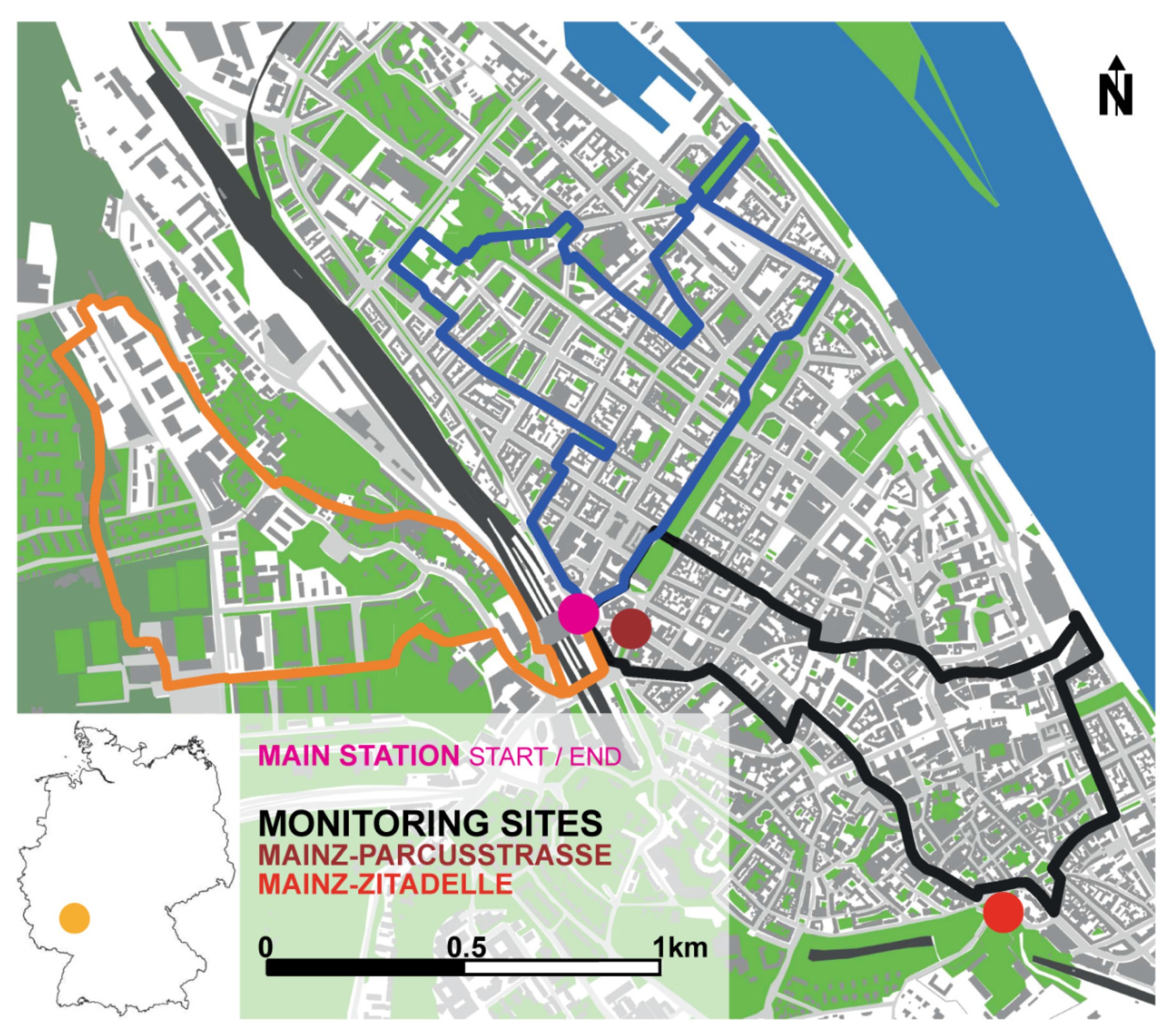
The study route includes three urban quarters of different characteristics: Altstadt, Hartenberg, and Neustadt (Figure 1). The Altstadt quarter is the old part of the town characterized by compact low- to midrise buildings, mostly paved streets, and pedestrian zones [31]. The urban architecture of the Hartenberg quarter, on the contrary, is a district with open low- to midrise buildings, a small grove, and low motorized traffic. The Neustadt quarter is characterized by mainly five-story-high buildings and narrow streets (~10 m wide), small parks (<150 m across), and low traffic intensity in a grid-based street layout. Large multi-lane roads with high traffic intensities surround this quarter as well as the Altstadt.
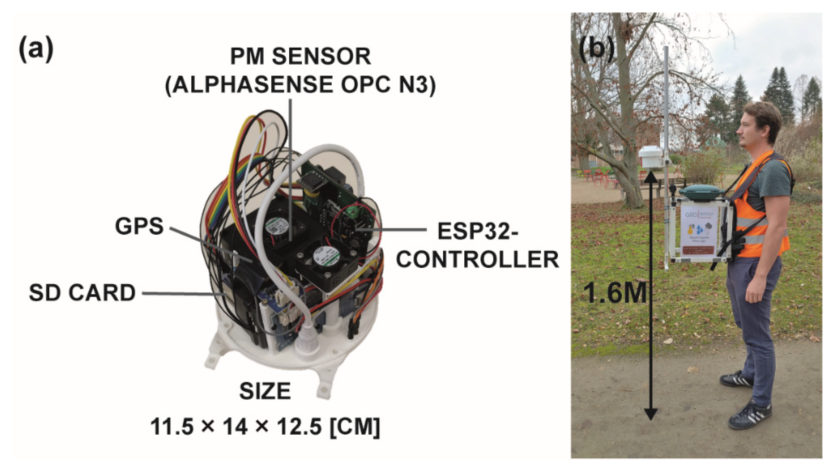
The total length of the study route was ~15 km or ~3 h walking by foot. To mitigate potential changes of local concentrations during such a long time span, we divided the route into three circular tracks, each leading through one of the districts. Each track was 5 km long (~1 h by foot) and shared the same starting and ending point at the Mainz train station (50.0017° N, 8.2595° E; Figure 1 magenta dot). The division into district tracks also supported multiple measurements per day. We conducted four measurement runs on each track, before and during the morning and afternoon rush hours starting at 6 a.m., 07:30 a.m., 4 p.m. and 05:30 p.m., with the exception of 14 September 2020 when we only measured in the afternoon. For each track, one device was used comprised of a PM sensor Alphasense OPC-N3 [22], a ESP32 controller [32], a GPS module [33], and a microSD card to save measurement data (Figure 2a). The sensors were mounted at adult breath height (1.6 m) on the front of a wearable rack to reduce influences of the person carrying the device (Figure 2b). To support the detection of local emitters during post-processing, every run was filmed with a camera attached to the rack.
2.2. Inter-Sensor Variability
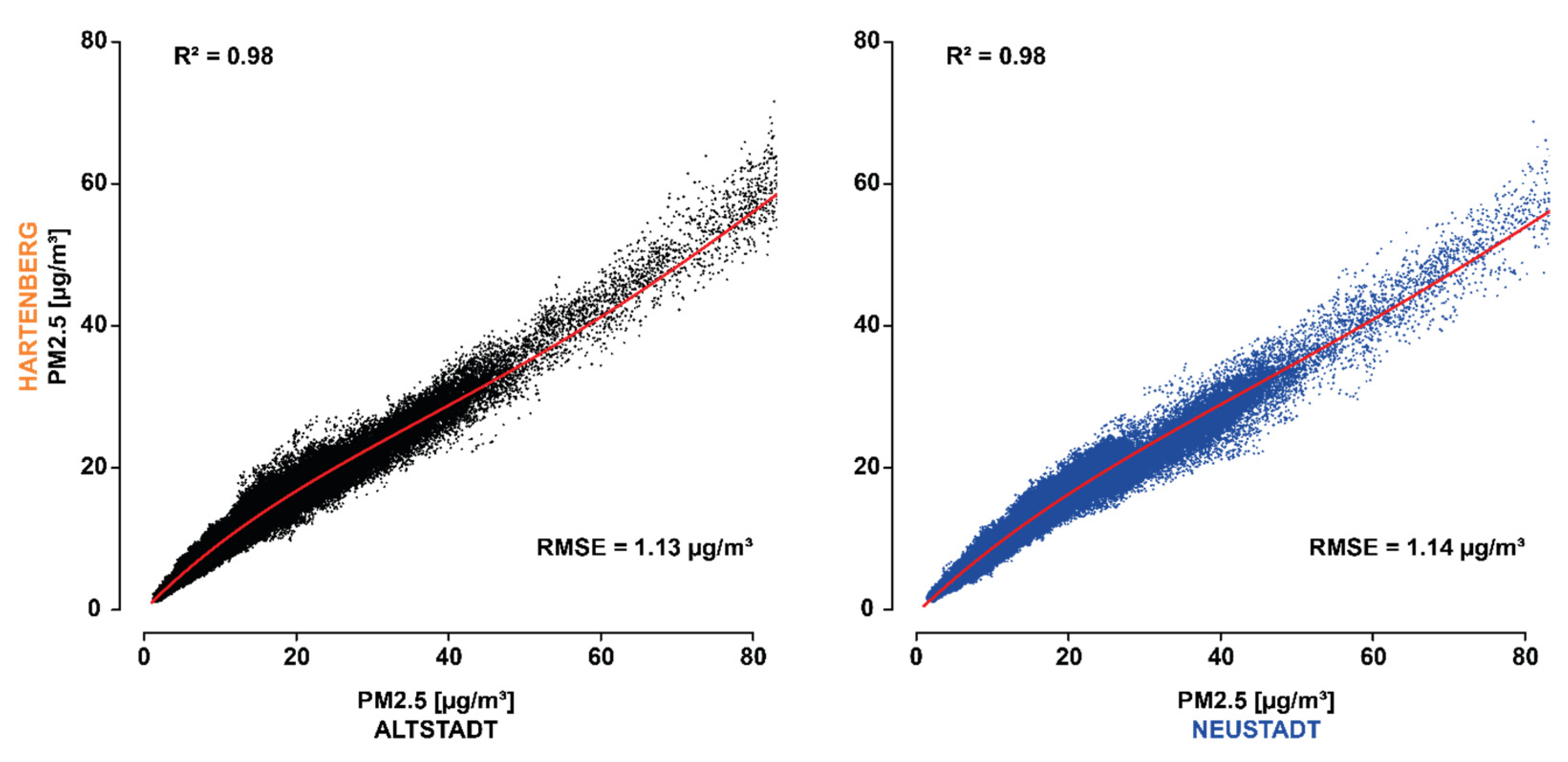
The Alphasense OPC-N3 sensors are low-cost optical particle counters following a light scattering principle [34]. The detected particles are put into bins considering their estimated size [35] and subsequently converted into mass concentrations [36]. The measurement range of the Alphasense OPC-N3 for particles is 0.35 to 40 µm [22]. The handy OPC-N3 units are suitable for a mobile measurement rack, affordable (~300 €), and perform well under laboratory conditions [37] considering the European EN 481 standard and manufacture calibration [26]. However, to further assess accuracy and address inter-sensor variability, a stationary field calibration in an environment similar to the study area is recommended [19,20,38,39,40,41]. Such a calibration was conducted on the Hartenberg district from 18–22 November 2020, 5–8 January 2021, and 20–23 February 2021. Since there were no reference devices that feature a comparable temporal resolution (<20 s), we adjusted two PM sensors to one other sensor: in our case, the sensors used in the Altstadt and Neustadt were adjusted to the Hartenberg sensor (Figure 3). The devices were co-located on the same height side-by-side to measure PM2.5 concentrations in a 1 s interval. The resulting data were then processed into 20 s arithmetic means, whereby the 10% highest and lowest values were truncated to mitigate the influence of short-term emissions (e.g., smokers).
Scatterplots of data measured in the Altstadt and Neustadt compared to Hartenberg showed that the cross-sensor accuracy was high. In addition to an explained variance exceeding 0.98, the data were homoscedastic and low root mean square errors reached 1.13 µg/m3 and 1.14 µg/m3, respectively. However, 4th degree polynomial (instead of linear) regression models were most suited to transform the measurements and produce statistically reliable data.
2.3. Data Post-Processing
To enable the comparison across different runs and tracks, several steps of post-processing had to be undertaken. At first, the recorded 1 s interval PM datasets were averaged calculating moving 20 s truncated arithmetic means, similar to the procedure used for calibration. A spatial synchronization of the data of the individual tracks was applied to adjust slight variations in run duration and minor inaccuracies of the GPS data. This was done by manually setting an ideal route for every sub-track and converting the data into points with a distance of 50 cm to each other. Each point was allocated to its appropriate data by calculating an average of the 10 closest original datapoints using an inverse distance weighting method [42]. The data of each track and run were then converted considering the polynomial regression equation obtained from the calibration trials. To reduce the effect of particle hygroscopy, a humidity correction for data recorded at RH > 60% according to Crilley et al. [26] was applied. The correction formula is based on the κ-Köhler theory, with κ = 0.33 as a composition of hygroscopic particles in the ambient air and a dry particle density of 1.65 g/cm3 [39]. Ambient RH measurements were taken from the long-term station Mainz-Zitadelle of the ZIMEN network. The processed data were then analyzed using descriptive statistics, i.e., arithmetic mean, median, and standard deviation (SD). In order to validate our absolute PM2.5 measurements for PM2.5 hotspot identification, a comparison of the mean PM2.5 values of each track and run in September and March against the regular long-term station data from Mainz-Parcusstraße, which is characterized by urban traffic, and Mainz Zitadelle, which resembles the urban background, was performed. These two measurement stations are part of the ZIMEN network, which carries out measurements with Thermo Fisher SHARP 5030 instruments [43] to monitor PM2.5 and PM10 on behalf of the state.
For the detection of highly polluted spots, the following steps were conducted. To counteract time-related fine particulate gradients, the data of each run were linearly detrended. Subsequently, the measurements of the simultaneously conducted runs in each district were combined and highly polluted locations (spots with 10% highest PM2.5 values) were identified: we determined highly polluted locations, for each period and season, by overlaying the extreme data of the respective runs and looking for matches. A match was recorded if the same location within a radius of 20 m indicated a pollution hot spot (i.e., 10% highest values) in several runs. After identifying highly polluted locations, we calculated PM2.5/PM10 ratios for the September and March data to evaluate emission sources.
3. Results and Discussion
3.1. Absolute PM2.5 Concentrations in September and March
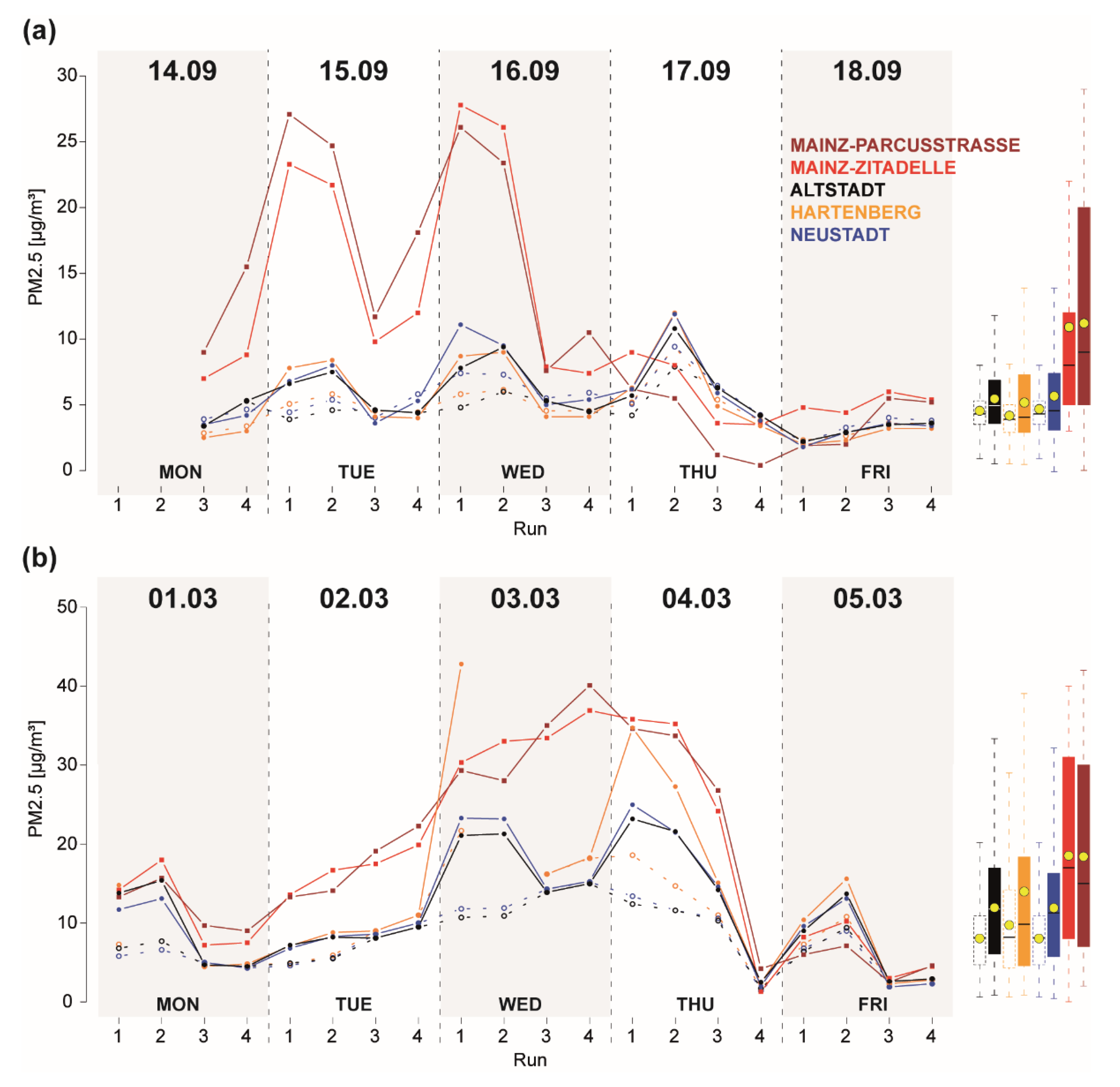
In September, the uncorrected mean PM2.5 concentrations were in line with the ZIMEN measurements and showed a diurnal pattern in PM2.5 characterized by 50 to 220% higher concentrations in the morning compared to the afternoon runs. This pattern was recorded during the first three days of the September campaign and followed by declining concentrations toward the end of the week (Figure 4, for median PM10 concentrations, see Figure S4).
This change in PM2.5 variability could be associated to changes in the weather regime: the first three days were characterized by warm late summer weather conditions consisting of high daily maximum air temperatures (TA) > 30 °C, moderate mean RH < 57%, and low maximum windspeeds < 1.0 m/s mainly from southeast directions (0; Figure S1). These stable conditions were also expressed by a low mean MLH < 200 m and high mean CIN with daily amplitudes up to 340 J/kg, which provided meteorologically favorable conditions for increased PM concentrations [14]. However, our measurements mainly underestimated the PM2.5 concentrations of the ZIMEN network in this period, particularly during the morning runs of 15 September 2020 and 16 September 2020 and after consideration of the humidity correction. These differences exceeded 23 µg/m3 in absolute values equal to 700% (both on 15 September 2020, first run). Right after the 4th run on 16 September 2020, the weather changed. Air pressure increased to 1015 hPa accompanied by rising windspeeds (max: <1.7 m/s), higher mean MLH value, lower CIN (69 J/kg), lower TA, and mean RH < 60% during last six runs of the September campaign which is why no humidity correction was applied for this period (Figure S1). During this time, the differences between our and the ZIMEN data decreased. Whereas our measurements showed still slightly higher PM2.5 concentrations on the 17th of September, differences did not exceed 3.0 µg/m3 thereafter.
In March, the PM2.5 concentrations were higher than in September. The differences between ZIMEN and our uncorrected measurements were moderate (<5.2 µg/m3) during the first four runs. Thereafter, when stable weather conditions set in (Table 1, Figure S2) and PM2.5 concentrations increased, a substantially larger underestimation up to 25.1 µg/m3 of the ZIMEN was recorded. An exception was run one on 3 March 2021 on the Hartenberg, where we measured >12 µg/m3 higher concentrations on average, though this seemed to be a single outlier that we could not explain. After 3 March 2021, the PM2.5 concentrations decreased due to a change in weather, upcoming north wind (max. 3.2 m/s), and a short-term shower, followed by decreasing of TA and RH. The differences between the ZIMEN measurements and those conducted by us were again small.
In both study periods, the differences in absolute PM2.5 between our runs and the stationary data were large and could not be explained by spatial variability. Our findings confirm the results of, e.g., Li et al. [45] and Sousan et al. [37], who identified this underestimation of OPC-N3 sensors compared to reference instruments. A stronger underestimation of the humidity-corrected PM2.5 concentration could be explained by the fact that any correction lowers the values [39]. Furthermore, the missing diurnal pattern during the first 3–4 days in September could be related to higher RH in the afternoon causing larger corrections. In March, however, the uncorrected measurements still showed diurnal patterns, whereas both the humidity-corrected and ZIMEN data did not. The humidity correction looked more suitable in the spring campaign, possibly because the prevailing higher RH resulted in corrections and hence stronger underestimations. The overall substantial underestimations and incomprehensible differences between mobile and stationary data led to the conclusion that our PM sensors cannot be used to assess absolute PM2.5 concentrations. For this reason, we used relative instead of absolute PM2.5 data to evaluate highly polluted areas.
3.2. Highly Polluted Places and Sources
The identification of highly polluted sites, i.e., sites with the highest 10% of PM2.5 concentrations throughout the entire study area, was conducted using 35 of 38 runs. Two runs were excluded due to sensor malfunctions (run two on 1 March 2021 and run two on 3 March 2021) and one run was omitted because of onsetting rain causing strongly lowered PM, which did not allow reasonable spatial comparisons of that run (run three on 4 March 2021).
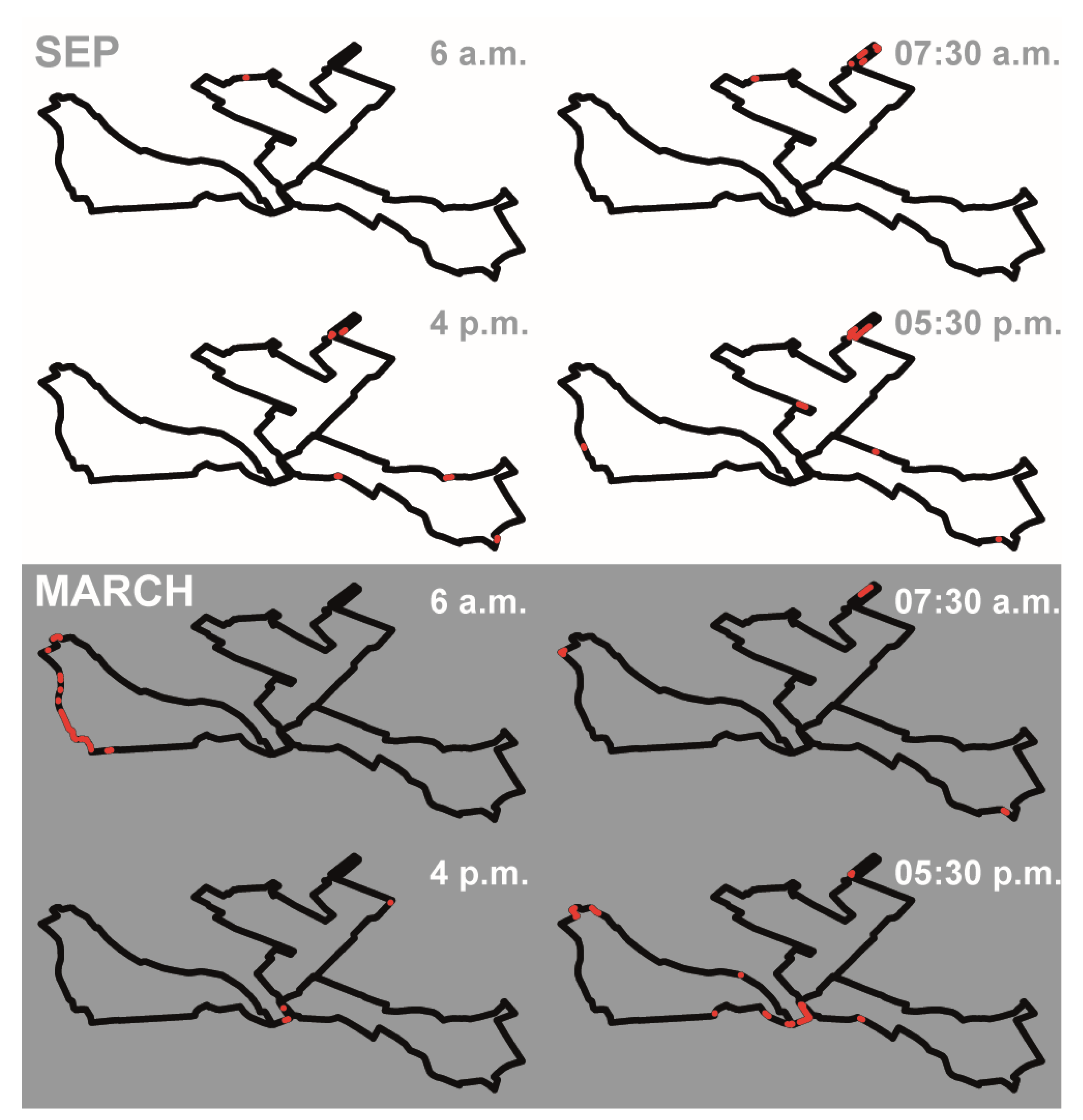
Our result showed that no location was consistently identified as a highly polluted area throughout the entire measurement period (Figure 5). This result was unexpected as our measurements took place along roads and large intersections with high vehicle traffic, reported to be main source of fine particle concentrations in urban areas [46]. On the contrary, locations with high levels of PM2.5 could be identified on all three tracks. While all PM2.5 hot spots were recorded in the Neustadt district during the September morning runs, the afternoon runs also included highly polluted places in the Altstadt. For the early morning runs in March, hot spots were solely detected in the Hartenberg, and in later runs, the highly polluted places were recorded on all tracks yet focused in the Hartenberg and Neustadt districts. People were thus exposed to high particle concentrations at varying places in different urban settings depending on the daytime and season.
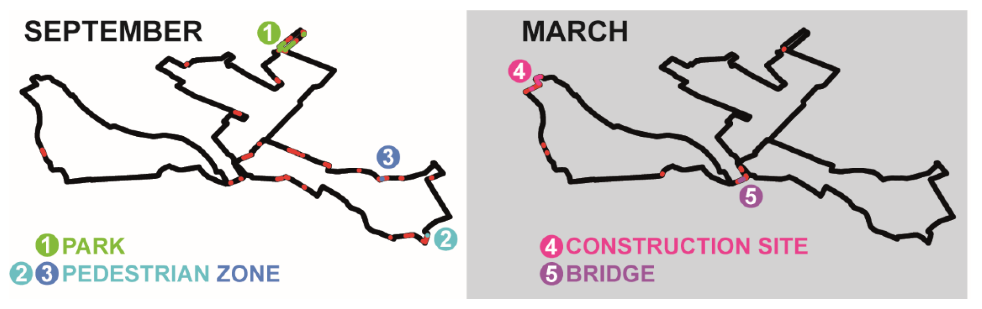
However, there were locations where pedestrians were exposed more frequently. In >50% of the September runs, we identified 21 different spots showing recurring high PM2.5 concentrations throughout all tracks (Figure 6, left panel). The larger number of hotspots in September could be assigned to the low absolute PM2.5 concentrations and minor differences among districts (Figure 4). At low particle concentrations, local emissions have a large influence on absolute PM2.5 peaks, and the mitigated track differences further the spread of hotspots. In March, there were at least seven highly polluted locations, mostly recorded on the overall more polluted Hartenberg track. However, when increasing the threshold to define highly polluted areas to >60% of the runs, the number of hot spots declined massively to only five locations (Figure 6, right panel; Figure S3). The remaining September hotspots were in a Neustadt park and the Altstadt pedestrian zone, whereas the two remaining March hotspots were located near a major housing construction site in Hartenberg and a traffic-loaded bridge near the train station.
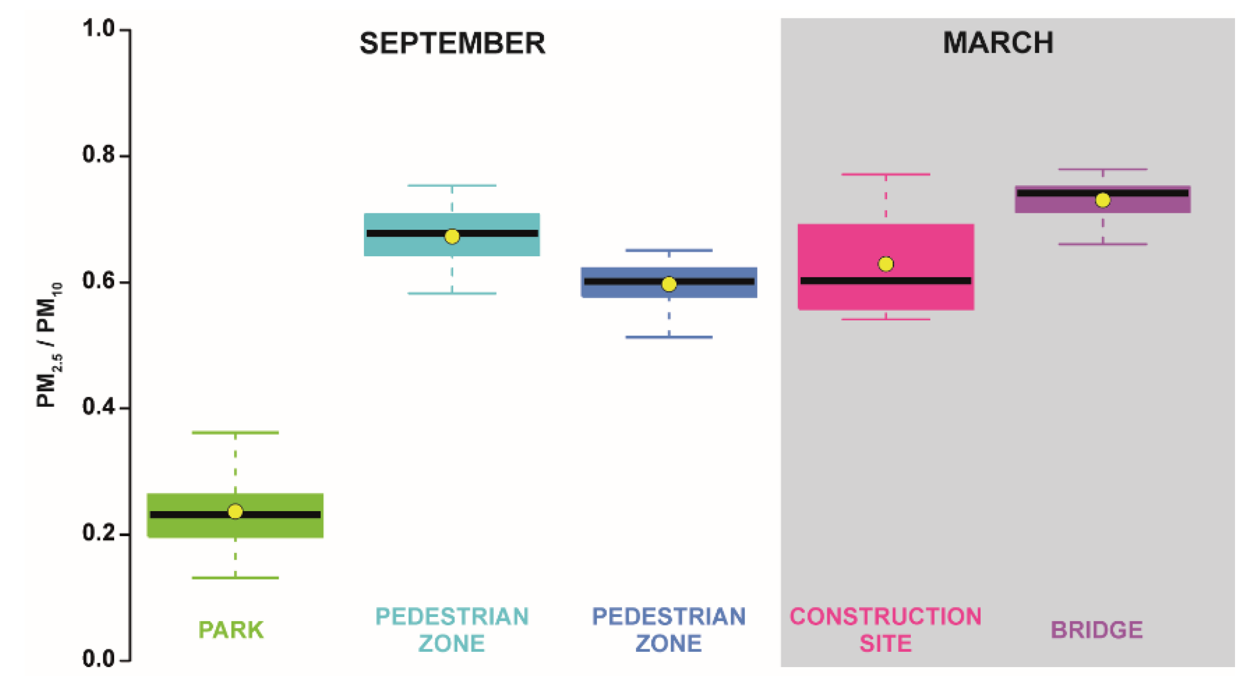
The March hotspots could clearly be attributed to anthropogenic sources: the origin of the particles at the bridge could be assigned to vehicles, as there was a high intensity of traffic on the multi-lane road crossing the bridge; the emission sources of the construction site was seemingly related to building processes and frequent construction vehicles [7,47]. These conclusions were supported by low apportionment of PM2.5 in PM10 at these locations (Figure 7). While the high PM2.5/PM10 ratio at the bridge near the main station (0.73) indicated the particle source to originate predominantly from anthropogenic emissions due to combustion processes of vehicles, the lower ratio (0.63) and high variability (interquartile range (IQR) = 0.13) at the construction sites pointed to a mixture of resuspended dust and particles from combustion processes.
The three September hotspots were particularly surprising, as there was no motorized traffic present at the time. This is in contrast to our hypothesis that the hotspots were related to heavy traffic streets as the main driver of high PM2.5 concentrations in urban areas [46]. The high values in the pedestrian zones could nevertheless be of anthropogenic origin, emitted by the exhaust systems of the restaurant kitchens blowing fine particles during deep-frying and roasting onto the streets [48]. Particles were likely additionally emitted in the outdoor areas of the restaurants (Figure S3, panel 3) due to smoking activities as reported by Birmili et al. [49]. High PM2.5/PM10 ratios >0.6 at these locations support the conclusion that anthropogenic sources were the main emitters, as does the fact that these sites were identified as PM2.5 hotspots in the afternoon runs, i.e., at times when restaurants were highly frequented.
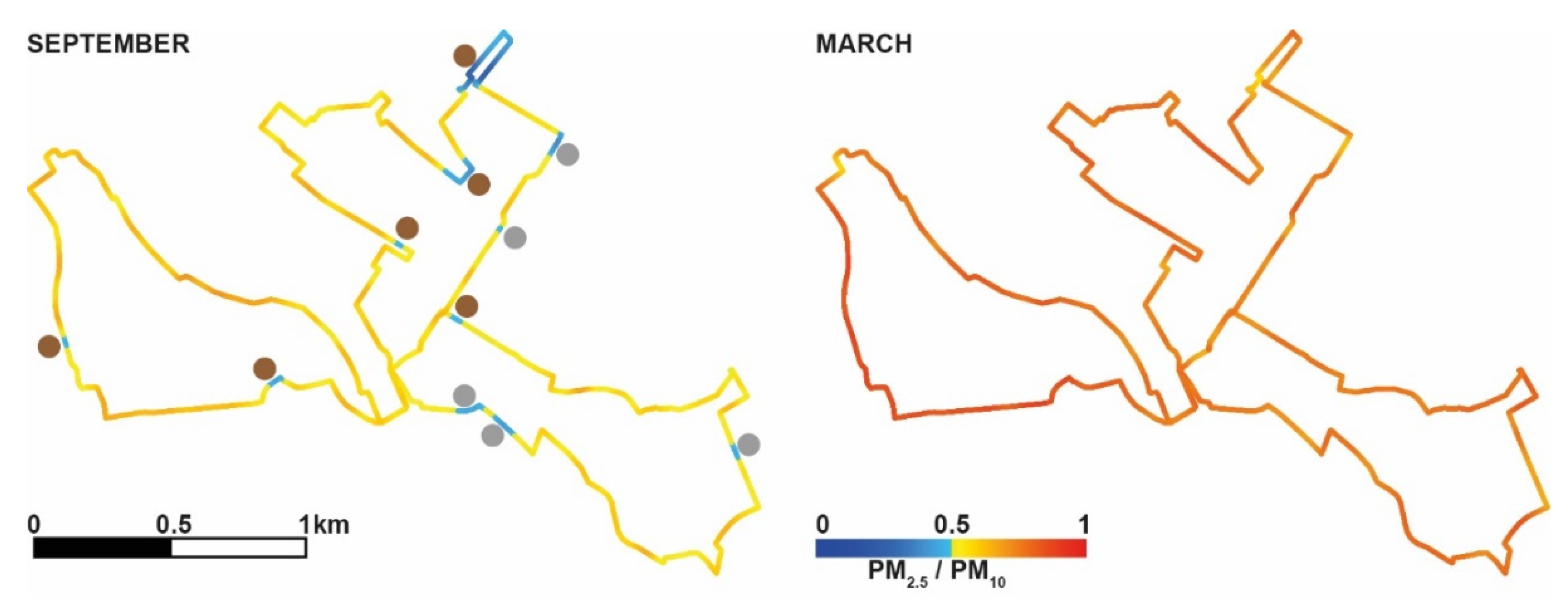
The particle sources in the park could not be attributed to combustion processes as in the other hotspots. The much lower mean PM2.5/PM10 ratio = 0.24 and small IQR = 0.07 pointed to a homogenous particle composition during September at this location (Figure 7). These values were either related to fugitive dust [11], i.e., impervious areas and footpaths containing loose top material, or to re-suspended road dust from the multi-lane road right next to the park. The spatial distribution of the PM2.5/PM10 ratios for September indicated that horizontal transport of fine particles from the close road was unlikely (Figure 8). Ratios <0.5 are rather indicative of locations with ongoing road and construction works and of parks with loose gravel on the walkways. Since there was no roadwork near to the park during the measurement campaign, whirled up dust from graveled and unpaved walkways was the most plausible local emissions. These findings corroborate with Paas and Schneider [50] who attributed higher mean concentrations in a green area to resuspended dried-out grass and unsurfaced footpath particles.
The comparison of highly polluted locations in September and March showed that the hotspots varied within the study area and that the underlying particle source changed. The data were additionally characterized by a substantial increase in PM2.5/PM10 ratios from 0.56 to 0.76 between autumn and spring, averaged over the study area (Figure 8). This seasonal change is in line with Speranza et al. [17] reporting ratios of <0.5 during warmer seasons (spring–summer) and ratio of >0.5 during colder seasons (autumn–winter). In our case, the increase in PM2.5 ratio was likely additionally affected by a pronounced cool thermal inversion (Table 1; Figure S2). These conditions constrained the vertical mixing of air, which led to an increase in fine particle concentrations at ground level. The prevailing low wind speeds subsequently amplified dry deposition of coarse particles, which in turn increased the PM2.5 apportionment in PM10 [51,52,53].
4. Conclusions
Using mobile low-cost devices containing Alphasense OPC-N3 sensors, small-scale PM2.5 hotspots along a 15 km transect in an urban area were identified. Three sensors showed a high agreement among each other but severely underestimated the measured PM2.5 concentrations of the ZIMEN network, particularly after applying a widely used humidity correction [39]. Absolute PM2.5 values were not considered, but additional calibration against high-resolution reference instruments could possibly improve the data accuracy of OPC-N3 sensors.
The identification of (relatively) heavily polluted locations revealed persisting PM2.5 hotspots in >60% of all runs, though the locations varied between the September and March study periods. The March hot spots were most likely triggered by local anthropogenic emissions including traffic emissions and construction work. This conclusion was supported by PM2.5/PM10 ratios >0.6 indicating combustion processes as the main particle source. The September hotspots, however, were located in areas dominated by pedestrians, and the PM sources were attributed to restaurant cooking exhaust air and outdoor seating activities. Exceptionally low PM2.5/PM10 ratios of 0.24 recorded in a park pointed to particles originating from locally emitted natural dust from unpaved footpaths, bare soils, and gravel surfaces. The PM2.5/PM10 ratios also increased from September to March as additional heating due to cooler temperatures and stable weather conditions prevailed during the spring campaign. The composition of sources can be further differentiated by analyzing the chemical composition of particles, which we recommend for further studies. The work detailed here revealed the capability of low-cost sensors to identify small-scale PM2.5 hotspots and sources. While the accuracy of absolute PM2.5 concentrations was insufficient, highly resolved spatiotemporal measurements may complement the stationary data and support the identification of highly polluted areas in the urban environment.
Supplementary Materials
The following supporting information can be downloaded at: https://www.mdpi.com/article/10.3390/atmos13050694/s1, Figure S1: weather conditions during September measurement period; Figure S2: weather conditions during March measurement period; Figure S3: Pictures of the high polluted areas. Figure S4: Mean PM10 concentrations in the Altstadt, Hartenberg, Neustadt and ZIMEN data.
Author Contributions
Conceptualization, L.H. and J.E.; methodology, L.H., T.S. and J.E.; formal analysis, L.H. and T.S.; investigation, L.H.; data curation, L.H.; writing—original draft preparation, L.H.; writing—review and editing, T.S. and H.S.; visualization, L.H.; supervision, J.E. All authors have read and agreed to the published version of the manuscript.
Funding
J.E. received support from the Gutenberg Research College, SustES (CZ.02.1.01/0.0/0.0/16_019/0000797), and ERC (AdG 882727).
Institutional Review Board Statement
Not applicable.
Informed Consent Statement
Not applicable.
Data Availability Statement
Not applicable.
Acknowledgments
We thank several students of the Johannes Gutenberg University in Mainz including Joelle Juretzek, Leonard Köster, and Jan-Erik Schmitz for supporting the mobile measurements. We are grateful to the environmental state office of Rhineland-Palatinate, particularly Michael Weißenmayer and Margit von Döhren from Referat 60 and Matthias Zimmer and Matthias Voigt from Referat 63, for providing data of the official meteorological measurement stations and radiometer as shown in Table 1, Figure 4, Figure 5, Figures S1 and S2.
Conflicts of Interest
The authors declare no conflict of interest.
References
- Mirabelli, M.C.; Ebelt, S.; Damon, S.A. Air Quality Index and air quality awareness among adults in the United States. Environ. Res. 2020, 183, 109185. [Google Scholar] [CrossRef]
- Maione, M.; Mocca, E.; Eisfeld, K.; Kazepov, Y.; Fuzzi, S. Public perception of air pollution sources across Europe. Ambio 2021, 50, 1150–1158. [Google Scholar] [CrossRef]
- Torres-Ramos, Y.D.; Montoya-Estrada, A.; Guzman-Grenfell, A.M.; Mancilla-Ramirez, J.; Cardenas-Gonzalez, B.; Blanco-Jimenez, S.; Sepulveda-Sanchez, J.D.; Ramirez-Venegas, A.; Hicks, J.J. Urban PM2.5 induces ROS generation and RBC damage in COPD patients. Front. Biosci. 2011, 3, 808–817. [Google Scholar] [CrossRef]
- Gualtieri, M.; Ovrevik, J.; Mollerup, S.; Asare, N.; Longhin, E.; Dahlman, H.-J.; Camatini, M.; Holme, J.A. Airborne urban particles (Milan winter-PM2.5) cause mitotic arrest and cell death: Effects on DNA, mitochondria, AhR binding and spindle organization. Mutat. Res. 2011, 713, 18–31. [Google Scholar] [CrossRef] [PubMed]
- Lelieveld, J.; Klingmüller, K.; Pozzer, A.; Pöschl, U.; Fnais, M.; Daiber, A.; Münzel, T. Cardiovascular disease burden from ambient air pollution in Europe reassessed using novel hazard ratio functions. Eur. Heart J. 2019, 40, 1590–1596. [Google Scholar] [CrossRef] [Green Version]
- Chen, L.C.; Lippmann, M. Effects of metals within ambient air particulate matter (PM) on human health. Inhal. Toxicol. 2009, 21, 1–31. [Google Scholar] [CrossRef] [PubMed]
- Karagulian, F.; Barbiere, M.; Kotsev, A.; Spinelle, L.; Gerboles, M.; Lagler, F.; Redon, N.; Crunaire, S.; Borowiak, A. Review of the Performance of Low-Cost Sensors for Air Quality Monitoring. Atmosphere 2019, 10, 506. [Google Scholar] [CrossRef] [Green Version]
- Schlesinger, R.B. The health impact of common inorganic components of fine particulate matter (PM2.5) in ambient air: A critical review. Inhal. Toxicol. 2007, 19, 811–832. [Google Scholar] [CrossRef] [PubMed]
- Xu, G.; Jiao, L.; Zhang, B.; Zhao, S.; Yuan, M.; Gu, Y.; Liu, J.; Tang, X. Spatial and Temporal Variability of the PM2.5/PM10 Ratio in Wuhan, Central China. Aerosol Air Qual. Res. 2017, 17, 741–751. [Google Scholar] [CrossRef] [Green Version]
- Parkhurst, W.J.; Tanner, R.L.; Weatherford, F.P.; Valente, R.J.; Meagher, J.F. Historic PM2.5/PM10 Concentrations in the Southeastern United States-Potential Implications of the Revised Particulate Matter Standard. J. Air Waste Manag. Assoc. 1999, 49, 1060–1067. [Google Scholar] [CrossRef]
- Evagelopoulos, V.; Zoras, S.; Triantafyllou, A.G.; Albanis, T.A. PM10–PM2.5 Time Series and Fractal Analysis. Glob. NEST J. 2019, 8, 234–240. [Google Scholar] [CrossRef]
- Querol, X.; Alastuey, A.; Rodriguez, S.; Plana, F.; Ruiz, C.R.; Cots, N.; Massague, G.; Puig, O. PM10 and PM2.5 source apportionment in the Barcelona Metropolitan area, Catalonia, Spain. Atmos. Environ. 2001, 35, 6407–6419. [Google Scholar] [CrossRef]
- Czernecki, B.; Półrolniczak, M.; Kolendowicz, L.; Marosz, M.; Kendzierski, S.; Pilguj, N. Influence of the atmospheric conditions on PM10 concentrations in Poznań, Poland. J. Atmos. Chem. 2017, 74, 115–139. [Google Scholar] [CrossRef] [Green Version]
- Graham, A.M.; Pringle, K.J.; Arnold, S.R.; Pope, R.J.; Vieno, M.; Butt, E.W.; Conibear, L.; Stirling, E.L.; McQuaid, J.B. Impact of weather types on UK ambient particulate matter concentrations. Atmos. Environ. X 2020, 5, 100061. [Google Scholar] [CrossRef]
- Wagner, P.; Schäfer, K. Influence of mixing layer height on air pollutant concentrations in an urban street canyon. Urban Clim. 2017, 22, 64–79. [Google Scholar] [CrossRef]
- Tang, G.; Zhang, J.; Zhu, X.; Song, T.; Münkel, C.; Hu, B.; Schäfer, K.; Liu, Z.; Zhang, J.; Wang, L.; et al. Mixing layer height and its implications for air pollution over Beijing, China. Atmos. Chem. Phys. 2016, 16, 2459–2475. [Google Scholar] [CrossRef] [Green Version]
- Speranza, A.; Caggiano, R.; Margiotta, S.; Summa, V.; Trippetta, S. A clustering approach based on triangular diagram to study the seasonal variability of simultaneous measurements of PM10, PM2.5 and PM1 mass concentration ratios. Arab. J. Geosci. 2016, 9, 1–8. [Google Scholar] [CrossRef]
- ZIMEN.-Luft-Überwachung in Rheinland-Pfalz-: Zentrales Immissionsmessnetz-ZIMEN-. Available online: https://luft.rlp.de/de/startseite/ (accessed on 2 March 2022).
- WMO. Low-Cost Sensors for the Measurement of Atmospheric Composition: Overview of Topic and Future Applications. 2018. Available online: https://www.ccacoalition.org/en/resources/low-cost-sensors-measurement-atmospheric-composition-overview-topic-and-future (accessed on 21 January 2022).
- Alfano, B.; Barretta, L.; Del Giudice, A.; de Vito, S.; Di Francia, G.; Esposito, E.; Formisano, F.; Massera, E.; Miglietta, M.L.; Polichetti, T. A Review of Low-Cost Particulate Matter Sensors from the Developers’ Perspectives. Sensors 2020, 20, 6819. [Google Scholar] [CrossRef]
- Al-Ali, A.R.; Zualkernan, I.; Aloul, F. A Mobile GPRS-Sensors Array for Air Pollution Monitoring. IEEE Sens. J. 2010, 10, 1666–1671. [Google Scholar] [CrossRef]
- Alphasense. Technical Information Release December 2018: Alphasense Particle Counter OPC-N Range Product Update. Available online: http://www.alphasense.com/WEB1213/wp-content/uploads/2019/02/OPC-N3-information-update-Dec-18.pdf (accessed on 1 April 2021).
- Morawska, L.; Thai, P.K.; Liu, X.; Asumadu-Sakyi, A.; Ayoko, G.; Bartonova, A.; Bedini, A.; Chai, F.; Christensen, B.; Dunbabin, M.; et al. Applications of low-cost sensing technologies for air quality monitoring and exposure assessment: How far have they gone? Environ. Int. 2018, 116, 286–299. [Google Scholar] [CrossRef]
- Sousan, S.; Koehler, K.; Hallett, L.; Peters, T.M. Evaluation of the Alphasense Optical Particle Counter (OPC-N2) and the Grimm Portable Aerosol Spectrometer (PAS-1.108). Aerosol Sci. Technol. 2016, 50, 1352–1365. [Google Scholar] [CrossRef] [PubMed]
- Brattich, E.; Bracci, A.; Zappi, A.; Morozzi, P.; Di Sabatino, S.; Porcù, F.; Di Nicola, F.; Tositti, L. How to Get the Best from Low-Cost Particulate Matter Sensors: Guidelines and Practical Recommendations. Sensors 2020, 20, 3073. [Google Scholar] [CrossRef] [PubMed]
- Crilley, L.R.; Shaw, M.; Pound, R.; Kramer, L.J.; Price, R.; Young, S.; Lewis, A.C.; Pope, F.D. Evaluation of a low-cost optical particle counter (Alphasense OPC-N2) for ambient air monitoring. Atmos. Meas. Tech. 2018, 11, 709–720. [Google Scholar] [CrossRef] [Green Version]
- Di Antonio, A.; Popoola, O.A.M.; Ouyang, B.; Saffell, J.; Jones, R.L. Developing a Relative Humidity Correction for Low-Cost Sensors Measuring Ambient Particulate Matter. Sensors 2018, 18, 2790. [Google Scholar] [CrossRef] [Green Version]
- ZIMEN. Jahresbericht 2020: Zentrales Immissionsmessnetz-ZIMEN-. Available online: https://luft.rlp.de/fileadmin/luft/ZIMEN/Jahresberichte/ZIMEN-Jahresbericht_2020.pdf (accessed on 20 January 2022).
- Deutscher Wetterdienst. Niederschlag: Vieljährige Mittelwerte 1981–2010. Available online: https://www.dwd.de/DE/leistungen/klimadatendeutschland/mittelwerte/nieder_8110_fest_html.html?view=nasPublication&nn=16102 (accessed on 10 May 2021).
- Deutscher Wetterdienst. Temperatur: Vieljährige Mittelwerte 1981–2010. Available online: https://www.dwd.de/DE/leistungen/klimadatendeutschland/mittelwerte/temp_8110_fest_html.html%3Fview%3DnasPublication (accessed on 10 May 2021).
- Stewart, I.D.; Oke, T.R. Local Climate Zones for Urban Temperature Studies. Bull. Am. Meteorol. Soc. 2012, 93, 1879–1900. [Google Scholar] [CrossRef]
- Espressif. ESP32. Available online: https://www.espressif.com/en/products/socs/esp32 (accessed on 5 February 2021).
- Simcom. Sim28. Available online: https://www.simcom.com/product/SIM28.html (accessed on 5 February 2021).
- Mie, G. Beiträge zur Optik trüber Medien, speziell kolloidaler Metallösungen. Ann. Phys. 1908, 330, 377–445. [Google Scholar] [CrossRef]
- Bohren, C.F.; Huffman, D.R. Absorption and Scattering of Light by Small Particles; Wiley: Hoboken, NJ, USA, 1998; ISBN 9780471293408. [Google Scholar]
- Walser, A.; Sauer, D.; Spanu, A.; Gasteiger, J.; Weinzierl, B. On the parametrization of optical particle counter response including instrument-induced broadening of size spectra and a self-consistent evaluation of calibration measurements. Atmos. Meas. Tech. 2017, 10, 4341–4361. [Google Scholar] [CrossRef] [Green Version]
- Sousan, S.; Regmi, S.; Park, Y.M. Laboratory Evaluation of Low-Cost Optical Particle Counters for Environmental and Occupational Exposures. Sensors 2021, 21, 4146. [Google Scholar] [CrossRef]
- Gysel, M.; Crosier, J.; Topping, D.O.; Whitehead, J.D.; Bower, K.N.; Cubison, M.J.; Williams, P.I.; Flynn, M.J.; McFiggans, G.B.; Coe, H. Closure study between chemical composition and hygroscopic growth of aerosol particles during TORCH2. Atmos. Chem. Phys. 2007, 7, 6131–6144. [Google Scholar] [CrossRef] [Green Version]
- Crilley, L.R.; Singh, A.; Kramer, L.J.; Shaw, M.D.; Alam, M.S.; Apte, J.S.; Bloss, W.J.; Hildebrandt Ruiz, L.; Fu, P.; Fu, W.; et al. Effect of aerosol composition on the performance of low-cost optical particle counter correction factors. Atmos. Meas. Tech. 2020, 13, 1181–1193. [Google Scholar] [CrossRef] [Green Version]
- Hagler, G.S.W.; Williams, R.; Papapostolou, V.; Polidori, A. Air Quality Sensors and Data Adjustment Algorithms: When Is It No Longer a Measurement? Environ. Sci. Technol. 2018, 52, 5530–5531. [Google Scholar] [CrossRef] [PubMed] [Green Version]
- Chatzidiakou, L.; Krause, A.; Popoola, O.A.M.; Di Antonio, A.; Kellaway, M.; Han, Y.; Squires, F.A.; Wang, T.; Zhang, H.; Wang, Q.; et al. Characterising low-cost sensors in highly portable platforms to quantify personal exposure in diverse environments. Atmos. Meas. Tech. 2019, 12, 4643–4657. [Google Scholar] [CrossRef] [Green Version]
- Shepard, D. A two-dimensional interpolation function for irregularly-spaced data. In Proceedings of the 1968 23rd ACM national conference, New York, NY, USA, 27–29 August 1968; Blue, R.B., Rosenberg, A.M., Eds.; ACM Press: New York, NY, USA, 1968; pp. 517–524. [Google Scholar]
- Thermo Fisher Science. Model 5030i SHARP: Instruction Manual. Available online: https://tools.thermofisher.com/content/sfs/manuals/EPM-manual-Model%205030i%20SHARP.pdf (accessed on 31 January 2022).
- Umweltmeteorologie RLP. Available online: https://luft.rlp.de/de/umweltmeteorologie/ (accessed on 1 March 2022).
- Li, J.; Mattewal, S.K.; Patel, S.; Biswas, P. Evaluation of Nine Low-cost-sensor-based Particulate Matter Monitors. Aerosol Air Qual. Res. 2020, 20, 254–270. [Google Scholar] [CrossRef] [Green Version]
- Kumar, P.; Rivas, I.; Sachdeva, L. Exposure of in-pram babies to airborne particles during morning drop-in and afternoon pick-up of school children. Environ. Pollut. 2017, 224, 407–420. [Google Scholar] [CrossRef] [PubMed]
- Yue, D.L.; Hu, M.; Wu, Z.J.; Guo, S.; Wen, M.T.; Nowak, A.; Wehner, B.; Wiedensohler, A.; Takegawa, N.; Kondo, Y.; et al. Variation of particle number size distributions and chemical compositions at the urban and downwind regional sites in the Pearl River Delta during summertime pollution episodes. Atmos. Chem. Phys. 2010, 10, 9431–9439. [Google Scholar] [CrossRef] [Green Version]
- Kang, K.; Kim, H.; Kim, D.D.; Lee, Y.G.; Kim, T. Characteristics of cooking-generated PM10 and PM2.5 in residential buildings with different cooking and ventilation types. Sci. Total Environ. 2019, 668, 56–66. [Google Scholar] [CrossRef]
- Birmili, W.; Rehn, J.; Vogel, A.; Boehlke, C.; Weber, K.; Rasch, F. Micro-scale variability of urban particle number and mass concentrations in Leipzig, Germany. METZ 2013, 22, 155–165. [Google Scholar] [CrossRef]
- Paas, B.; Schneider, C. A comparison of model performance between ENVI-met and Austal2000 for particulate matter. Atmos. Environ. 2016, 145, 392–404. [Google Scholar] [CrossRef]
- Huang, R.-J.; Zhang, Y.; Bozzetti, C.; Ho, K.-F.; Cao, J.-J.; Han, Y.; Daellenbach, K.R.; Slowik, J.G.; Platt, S.M.; Canonaco, F.; et al. High secondary aerosol contribution to particulate pollution during haze events in China. Nature 2014, 514, 218–222. [Google Scholar] [CrossRef] [Green Version]
- Wallace, J.; Kanaroglou, P. The effect of temperature inversions on ground-level nitrogen dioxide (NO2) and fine particulate matter (PM2.5) using temperature profiles from the Atmospheric Infrared Sounder (AIRS). Sci. Total Environ. 2009, 407, 5085–5095. [Google Scholar] [CrossRef]
- Blanco-Becerra, L.C.; Gáfaro-Rojas, A.I.; Rojas-Roa, N.Y. Influence of precipitation scavenging on the PM2.5PM10 ratio at the Kennedy locality of Bogotá, Colombia. Rev. Fac. Ing. Antioq. 2015, 76, 58–65. [Google Scholar] [CrossRef]
Figure 1.
Study tracks in the Mainz Altstadt, Hartenberg, and Neustadt (black, orange, and blue lines, respectively), their joint start and end point at the main station (magenta), and the monitoring sites of the ZIMEN network at Mainz-Parcusstraße (dark red) and Mainz-Zitadelle (red) of the ZIMEN network, and map of Germany showing the location of Mainz (orange).

Figure 2.
(a) Design and components of the measurement device (dimensions: 11.5 cm × 14 cm × 12.5 cm), and (b) picture of a person carrying the rack.
Figure 2.
(a) Design and components of the measurement device (dimensions: 11.5 cm × 14 cm × 12.5 cm), and (b) picture of a person carrying the rack.

Figure 3.
Scatter plots and polynomial regressions of the moving 20 s truncated arithmetic mean PM2.5 adjustments of the sensors used on the Altstadt (left panel) and Neustadt tracks (right panel) to the Hartenberg sensor including R2 coefficients and root mean square errors for the adjustment periods from 18–22 November 2020, 5–8 January 2021, and 20–23 February 2021.

Figure 4.
Mean PM2.5 concentrations in the Altstadt, Hartenberg, Neustadt (black, blue, and orange colors, respectively), and ZIMEN data from the Mainz-Parcusstraße and Mainz-Zitadelle (dark red and red colors, respectively) during the study periods in (a) September and (b) March with corresponding boxplots and arithmetic means (yellow dots). The unfilled dots symbolize the humidity-corrected PM2.5 measurements, and the filled dots symbolize PM2.5 concentrations without humidity correction.

Figure 5.
Locations showing the 10% highest PM2.5 concentrations (red dots) throughout the runs during the September and March campaigns.
Figure 5.
Locations showing the 10% highest PM2.5 concentrations (red dots) throughout the runs during the September and March campaigns.

Figure 6.
Locations with 10% highest PM2.5 concentrations in >60% of all runs in September (left panel) and March (right panel). Colors refer to parks (green), pedestrian zone (blue and cyan), construction site (magenta), and a bridge (violet).
Figure 6.
Locations with 10% highest PM2.5 concentrations in >60% of all runs in September (left panel) and March (right panel). Colors refer to parks (green), pedestrian zone (blue and cyan), construction site (magenta), and a bridge (violet).

Figure 7.
PM2.5/PM10—ratio boxplots of the PM2.5 hot spots in the park (green) and pedestrian zones (cyan and blue) for September (green, cyan, and blue colors) and the construction site (magenta) and motorized road (violet) for March. Yellow dots indicate mean values.
Figure 7.
PM2.5/PM10—ratio boxplots of the PM2.5 hot spots in the park (green) and pedestrian zones (cyan and blue) for September (green, cyan, and blue colors) and the construction site (magenta) and motorized road (violet) for March. Yellow dots indicate mean values.

Figure 8.
Spatial patterns of mean PM2.5/PM10 ratios in September and March. Bluish colors indicate ratios between 0 to 0.5. The dots mark important particle sources including unpaved surfaces (brown) and construction sites (grey).
Figure 8.
Spatial patterns of mean PM2.5/PM10 ratios in September and March. Bluish colors indicate ratios between 0 to 0.5. The dots mark important particle sources including unpaved surfaces (brown) and construction sites (grey).


Table 1.
Meteorological conditions during the study measurement periods in September and March including mean air temperature (TA) (°C), mean relative humidity (RH) (%), precipitation sum (mm), atmospheric pressure (hPA), wind speed (m/s), wind direction (°), mean convective inhibition (CIN) (J/kg), and mean mixing layer height (MLH) (m). Adapted with permission from Refs. [18,44] 2021, Landesamt für Umwelt Rheinland-Pfalz.
| Date | 14.09. | 15.09. | 16.09. | 17.09. | 18.09. | 01.03. | 02.03. | 03.03. | 04.03. | 05.03. |
|---|---|---|---|---|---|---|---|---|---|---|
| TA (°C) | 23.0 | 23.3 | 23.8 | 19.5 | 18.8 | 7.7 | 9.2 | 8.2 | 9.6 | 5.8 |
| RH (%) | 53.6 | 56.6 | 57.1 | 51.2 | 46 | 66.8 | 62.7 | 71.5 | 71.7 | 59.4 |
| Precipitation (mm) | 0.3 | 0 | 0.1 | 1.1 | 1.9 | 0 | 0 | 0 | 9.5 | 0 |
| Atmospheric pressure (hPA) | 1013 | 1009 | 1007 | 1013 | 1012 | 1021 | 1020 | 1017 | 1008 | 1014 |
| Wind direction (°) | 56 | 63 | 147 | 105 | 100 | 143 | 122 | 148 | 225 | 166 |
| Wind speed (m/s) | 0.2 | 0.1 | 0.4 | 0.6 | 0.6 | 0.5 | 0.3 | 0.2 | 0.6 | 1.1 |
| CIN (J/kg) | 177 | 171 | 171 | 60 | 85 | 163 | 148 | 219 | 110 | 27 |
| MLH (m) | 170 | 165 | 115 | 312 | 249 | 135 | 163 | 102 | 226 | 455 |
Publisher’s Note: MDPI stays neutral with regard to jurisdictional claims in published maps and institutional affiliations. |
© 2022 by the authors. Licensee MDPI, Basel, Switzerland. This article is an open access article distributed under the terms and conditions of the Creative Commons Attribution (CC BY) license (https://creativecommons.org/licenses/by/4.0/).
Share and Cite
MDPI and ACS Style
Harr, L.; Sinsel, T.; Simon, H.; Esper, J. Seasonal Changes in Urban PM2.5 Hotspots and Sources from Low-Cost Sensors. Atmosphere 2022, 13, 694. https://doi.org/10.3390/atmos13050694
AMA Style
Harr L, Sinsel T, Simon H, Esper J. Seasonal Changes in Urban PM2.5 Hotspots and Sources from Low-Cost Sensors. Atmosphere. 2022; 13(5):694. https://doi.org/10.3390/atmos13050694
Chicago/Turabian StyleHarr, Lorenz, Tim Sinsel, Helge Simon, and Jan Esper. 2022. "Seasonal Changes in Urban PM2.5 Hotspots and Sources from Low-Cost Sensors" Atmosphere 13, no. 5: 694. https://doi.org/10.3390/atmos13050694
Note that from the first issue of 2016, this journal uses article numbers instead of page numbers. See further details here.