
Does Below-Above Canopy Air Mass Decoupling Impact Temperate Floodplain Forest CO2 Exchange?


Department of Matter and Energy Fluxes, Global Change Research Institute, Czech Academy of Sciences, Bělidla 986/4a, 603 00 Brno, Czech Republic
*
Author to whom correspondence should be addressed.
Atmosphere 2022, 13(3), 437; https://doi.org/10.3390/atmos13030437
Submission received: 31 January 2022
/
Revised: 1 March 2022
/
Accepted: 4 March 2022
/
Published: 8 March 2022
(This article belongs to the Special Issue Frontiers in Quantifying CO2 Uptake by Forests)
Abstract
:Environmental conditions influence forest ecosystems and consequently, its productivity. Thus, the quantification of forest CO2 exchange is a critical requirement to estimate the CO2 balance of forests on a local and regional scale. Besides interpreting the annual CO2 exchange corresponding to environmental conditions over the studied years (2015–2020) at the floodplain forest in Lanžhot, Czech Republic (48.6815483 N, 16.9463317 E), the influence of below-above canopy air mass decoupling on above canopy derived CO2 exchange is the focus of this study. For this purpose, we applied the eddy covariance (EC) method above and below the forest canopy, assessing different single- and two-level flux filtering strategies. We focused on one example year (2019) of concurrent below and above canopy EC measurements. We hypothesized that conventional single-level EC flux filtering strategies such as the friction velocity (u*) filtering approach might not be sufficient to fully capture the forest CO2 exchange at the studied ecosystem. Results suggest that decoupling occurs regularly, but the implication on the above canopy derived EC CO2 fluxes appears to be negligible on an annual scale. We attribute this to the open canopy and flat EC tower surrounding terrain which inhibits horizontal removal of below-canopy respired CO2.
1. Introduction
Floodplain forests play an important role in strong, mutual and continuous interaction between climate and the ecosystems, despite a relatively small total area of coverage in Europe [1]. They are characterized by a high production level and biodiversity [1,2]. Floodplain forests are able to store huge amounts of soil carbon [3]. Wetlands, to which floodplain forests belong, hold the majority of the global soil carbon pool [4]. Carbon dioxide (CO2) sequestration and storage is the result of the balance of gross primary production (GPP) (taking up CO2 for photosynthesis and producing organic matter), and ecosystem respiration, Reco (or decomposition; generating CO2 or methane from organic matter) [5]. On some wetlands, the decomposition is very slow, and when plant productivity exceeds it, carbon accumulates [6]. In the course of ongoing climate change with more often occurring extreme events, the role of floodplain forests as carbon stores and their role in nutrient cycles to mitigate climate change has become even more crucial [7,8,9,10]. Changing temperature and precipitation regimes due to changing climatic conditions can shift the balance between the rate of Reco and GPP, which can cause wetlands to become a carbon source [11,12].
The floodplain forest study site near Lanžhot, Czech Republic is a hydrologically controlled wetland ecosystem. Thus, changes in the environmental conditions at the study site might be man-made by artificial flooding, or induced by climate changes. Interpreting the annual CO2 exchange corresponding to environmental conditions in the course of the study at the floodplain forest in Lanžhot was one of our main interests. We focused on the quantification of Net Ecosystem CO2 Exchange (NEE) attributable to the floodplain forest near Lanžhot. This quantification is a critical requirement in order to estimate the CO2 balance on a local and regional scale.
Our main method of choice, the eddy covariance (EC) method, has become a key approach to assess the forest ecosystem CO2 exchange [13,14]. Through direct, precise and continuous measurements, EC provides the unique possibility to measure ecosystem-atmosphere turbulent exchange of matter and energy fluxes, e.g., CO2 fluxes. In the case of CO2, this flux equals NEE under optimal measurement conditions and on longer time scales (e.g., annual). Revealing the interactions between terrestrial biosphere and atmosphere on an ecosystem scale, NEE indicates if there is a carbon uptake or efflux in the studied ecosystem [15]. From NEE and accompanying environmental measurements, GPP and Reco can be derived [16].
Eddy covariance requires certain assumptions and preconditions to be fulfilled, e.g., steady-state conditions, well-developed turbulence, homogenous underlying vegetation and ideally, flat terrain [14]. Additionally, a number of corrections are necessary during the flux calculation process [13,17]. These preconditions are not always met. For example, low wind conditions and stable stratification across the canopy may lead to decoupling of the air masses close to the ground from the air masses above the canopy due to insufficient turbulent mixing. As NEE measurements are conducted only above the forest, respiration components from within and below canopy might be missing in the above canopy data under such insufficient mixing conditions. This leads to an overestimation of the carbon sink strength of the studied forest ecosystems [18,19,20,21,22], if the respired below canopy CO2 is removed from the probed measurement volume before reaching the above canopy instrumentation.
The most common approach to guarantee well-developed turbulence is the single-level friction velocity (u*) filtering approach [23,24,25,26]. Friction velocity is a measure of mechanical turbulence development and allows to discard measurements from weak turbulent periods which are potentially not fully representative for the whole ecosystem, and to replace them by gap-filled estimates obtained under well-developed turbulence conditions [27]. The estimation of a filtering threshold is site-specific and empirically determined by evaluating the relation between u* and nighttime above canopy CO2 fluxes under the assumption that nighttime above canopy CO2 fluxes become independent of u* at a certain threshold [28,29,30].
The problem of flux determination under poorly developed turbulence has been known for many years, however, all determining factors are not yet fully understood. In recent years, several case studies approached this topic by addressing canopy decoupling in forests. They aimed, inter alia, for testing and validating the applicability of the EC technique, assessing the spatial variability of subcanopy fluxes, evaluating the factors controlling these fluxes, or the improvement of the NEE estimates [20,22,31,32,33].
Some of these studies led to the conclusion that using the single-level u* filtering approach is not sufficient to define well-developed turbulent mixing between below and above canopy air masses [13,20,21,34]. Especially at tall and dense canopies, continuous decoupling of the sub-canopy layer from the overstory and above canopy air masses may occur due to stable stratification across the canopy and the mechanical barrier induced by the forest canopy [35].
Recently, as an alternative to the single-level u* filtering approach, a two-level filtering strategy has been proposed [20,32]. It can be applied both on the relation between u* above and u* below the canopy as well as on the relation between the standard deviation of the vertical wind speed above (σw_a) and below (σw_b) the canopy. Linear relation between u* above and below canopy (or σw_a and σw_b) reflects conditions when below and above canopy air masses are fully coupled. Thomas et al. [20] proposed ways to identify thresholds for both σw (or u*) above and below the canopy, above which full coupling is assumed. However, as micrometeorological conditions differ spatially and temporarily, individual threshold determination approaches might be applicable, even though general strategies are proposed [20,32]. For comparability reasons, the focus in the current study is on the u* thresholds as it gives the possibility to directly assess the decoupling effect in comparison to the most widely used standard method single-level u* filtering.
The application of concurrent EC below and above canopy at the studied floodplain forest promises new insights on the phenomenon of canopy decoupling and its potential influence on above canopy derived EC fluxes, as the study site is in very flat terrain. In this sense, the study site represents ideality.
Our specific aims are (1) to interpret the annual CO2 exchange corresponding to environmental conditions over the study years at the floodplain forest in Lanžhot and (2) to evaluate and assess different single- and two-level flux filtering strategies with regards to decoupling and its impact on above canopy derived forest CO2 exchange.
We hypothesized that conventional single-level EC flux filtering strategies like the u* filtering might not fully capture the forest CO2 exchange at the studied ecosystem.
2. Materials and Methods
2.1. Site Description and Characteristics
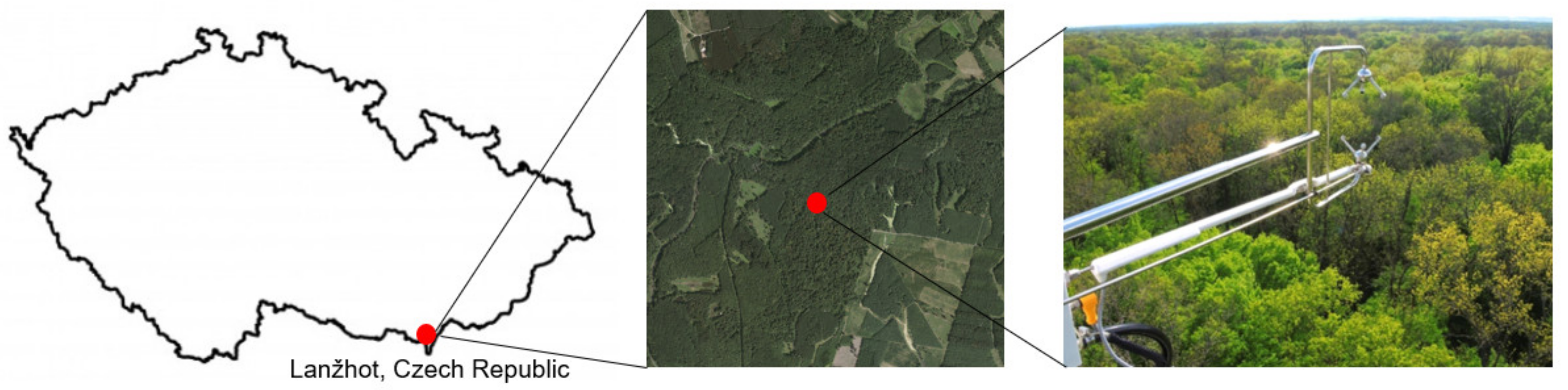
The studied lowland floodplain forest is situated 6.5 km north of the confluence of Morava and Thaya rivers (48.6815483 N, 16.9463317 E), on a flat surface area at elevation 150 m a.s.l. in the Czech Republic (Figure 1).
The long-term average annual precipitation is 517 mm and the mean annual temperature is 9.5 °C. The average groundwater level is −2.7 m. The last flood was in 2013 and only in the lowest parts of the studied site above the soil surface. The experimental site consisting of a 122 (in the year 2022) years-old forest is composed of typical hardwood species. The main tree species are English oak (Quercus robur L.), narrow-leaved ash (Fraxinus angustifolia Vahl) and hornbeam (Carpinus betulus L.) with average diameter at breast height (DBH ± standard deviation) of 51.8 (±12.3) cm, 56.4 (±9.2) cm and 27.7 (±11.2) cm [9]. The average stand height is 27 m and the average height of the three main species separately is 31.0 (±3.6) m for oak, 35.9 (±3.4) m for ash and 23.4 (±6.9) m for hornbeam. The predominant soil types are Eutric Humic Fluvisol, Haplic Fluvisol and Eutric Fluvisol (according FAO 2014 Classification) with minimal soil depth of 60 cm [36]. Rising air temperatures and decreasing water level depths can be observed in the study region which are likely caused by climate change. Additionally, hydrological management via building of artificial dams in the study region amplified the drying of the study site and yielded that natural flooding very rarely occurs nowadays. Consequently, the water regime of the site changed over the years and nowadays represents relatively dry conditions for a floodplain forest.
2.2. Instrumentation
Eddy covariance measurements
Two eddy covariance systems provided data to this study. The above canopy system was installed initially at a height of 44 m and on 5th December 2018 moved to 48 m above ground. The second system was installed below the canopy at a height of 3.5 m above ground. Both systems consisted of a Gill HS-50 sonic anemometer (Gill Instruments Limited, Hampshire, UK) for measuring the horizontal (u, v) and vertical (w) wind components as well as sonic temperature (Ts), and an LI-7200 (LI-COR Environmental, Lincoln, USA) gas analyzer for detecting H2O and CO2 mixing ratios (dry mole fraction). The sampling frequency of both systems was 20 Hz.
Environmental measurements
The instrumentation used in our study (Table 1) follows the standards of the Integrated Carbon Observation System (ICOS) which provides high-quality long-term observations of greenhouse gases (GHG) and greenhouse gas exchange https://www.icos-cp.eu/ (accessed on 5 March 2022) [37,38,39,40,41]. Vapor pressure deficit (VPD), later on used in the course of this study, was calculated using Tair and RH measurements.
2.3. Data Handling
2.3.1. Turbulent Flux Calculation and Post-Processing
Our whole analysis covers a multi-year period of EC measurements above the canopy (years 2015–2020), and a 1-year focal period (year 2019) with concurrent EC measurements above and below the canopy.
Standardly, vertical turbulent fluxes were calculated with EddyPro® (version 6.2.0, LI-COR Biosciences, Rockville, MD, USA) using the eddy covariance method (described in detail by [13,42]) both above and below the canopy with an averaging time of 30 min. The correct application of the EC method requires several corrections on the calculated covariances between vertical wind component w and the quantity of interest, e.g., CO2. The planar-fit method [43] was used to ensure that the long-term mean of individual vertical wind measurements w is negligible or nullified. Furthermore, a rotation into the main wind direction is conducted with this method. Potential flux losses in the high frequency range, e.g., due to path length averaging or the spatial separation of sonic measurement path and gas analyzer were accounted for with the correction proposed by [44]. Additionally, the measured buoyancy flux was converted into the real sensible heat flux according to [45]. The EC software also includes a quality flagging scheme testing the data for stationarity and development of turbulence and finally, providing an overall quality flag combining the results of both tests [46].
2.3.2. CO2 Flux Gap-Filling and Partitioning
Gaps in the time series of measured CO2 fluxes due to instrument malfunctioning or filtering strategies were filled using the R [47] package REddyProc [48] where a MDS (marginal distribution sampling) gap-filling algorithm is applied [30].
The CO2 flux partitioning in GPP and Reco was also carried out with REddyProc. We followed the “daytime” approach as proposed by [16]. This approach uses nighttime CO2 fluxes to infer the temperature sensitivity of Reco, but uses daytime data only to derive the light- and temperature-driven models for GPP and Reco, respectively [49].
2.3.3. Storage Flux Calculation
Changes in CO2 storage were calculated following the approach outlined in [50]:
where the integration is performed from the ground to the measurement height hm. Equation (1) describes the changes of CO2 concentrations (CO2) over time (t) along the measurement path (dz) from ground to uppermost measurement height.
We used the single-point version of Equation (1) which is assuming that all gradients nullify at ground level and that the profile is linear from the measurement point to the ground. These conditions are rarely met in reality. Even if this assumption can produce significant uncertainty on half-hourly storage fluxes, the effect of these errors of the single-point storage method is minor on long-term storage change estimates [51]. The single-point storage method is implemented in EddyPro which provides the data for our further storage flux analysis.
2.3.4. Filtering Approaches to Address Decoupling Effects on CO2 Fluxes
u* filtering
To derive the u* filtering thresholds, we applied the moving point test method [26] implemented in REddyProc on our data. This approach provides u* thresholds for seasons/temperature subclasses and finally aggregates these u* values also to a yearly threshold. The u* filtering was conducted on the already quality flag-filtered data.
u* two-level filtering
The two-level u* filtering method allowed us to detect whether air masses above and below the canopy are fully coupled or not. This filtering was applied on the already quality filtered data. We used the relation of above and below canopy u* as the decoupling indicator. When the relation is linear and both thresholds are met, the air masses above and below the canopy are fully coupled [20]. The filtering thresholds of u* above and below the canopy were derived following the procedure described by [21]. The above canopy u* threshold was verified by break point analysis applied on the relation between above and below canopy u* values, using the R [47] package segmented in its standard configuration.
2.3.5. Net Ecosystem CO2 Exchange
The net ecosystem CO2 exchange sums up via the three components of turbulent exchange, storage flux and advection [22]. By applying the two-level filtering proposed in Section 2.3.4 on EC data, we can assume that advection is negligible [20]. Storage fluxes, on the other hand, nullify over longer time periods [22]. Consequently, it is justified to assume that the EC measured turbulent flux is approximately equal to NEE, when used for decoupling filtered data and evaluating longer time periods.
According to the atmospheric sign convention, negative fluxes of NEE represent a carbon uptake period (CUP).
3. Results
3.1. Meteorological Conditions
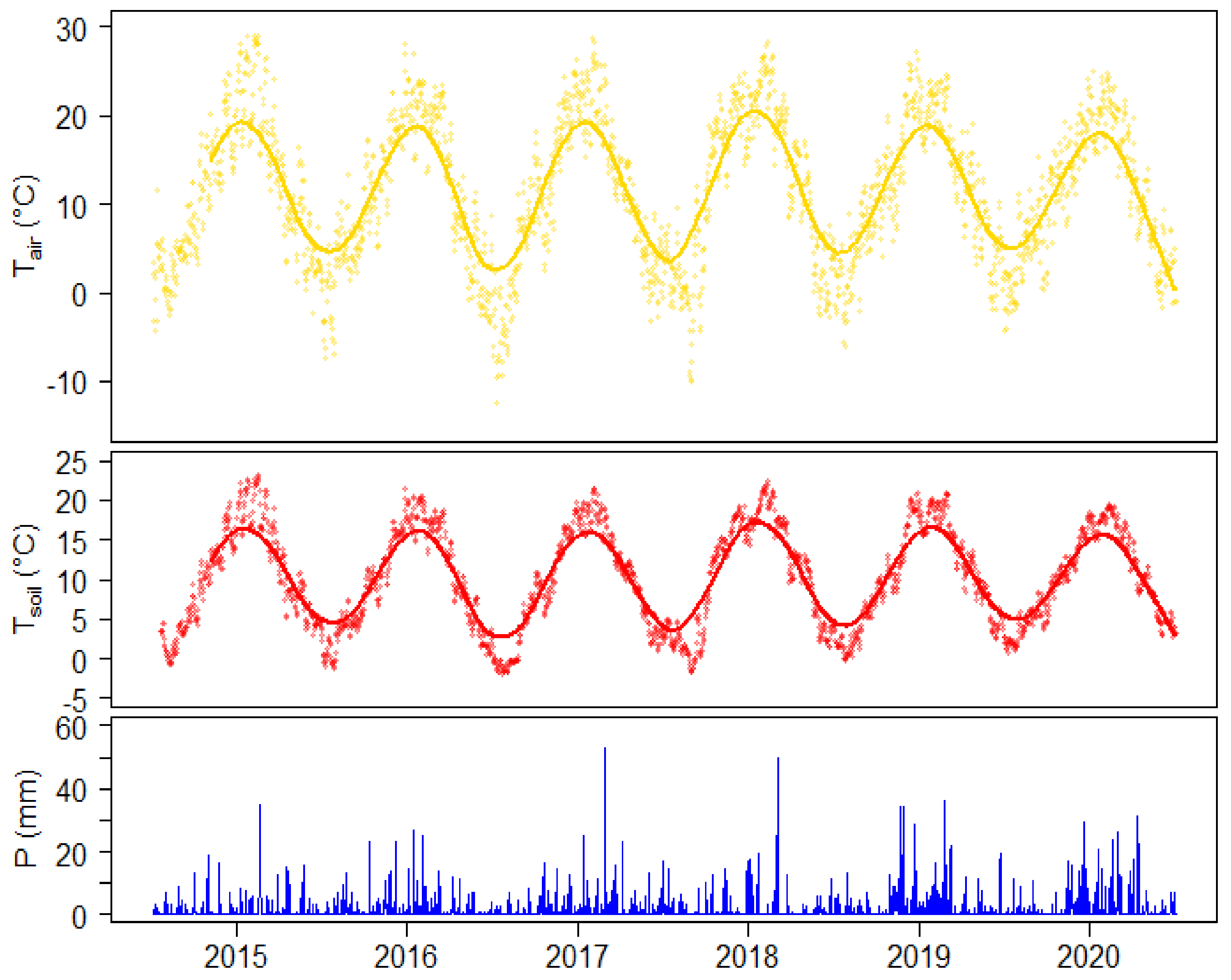
The study period (2015–2020) was characterized by an average air temperature of 11.4 °C, soil temperature of 10.2 °C and mean annual total precipitation of 517 mm. A detailed description of the particular years 2015–2018 is presented in [9]. In comparison with the most dry and hot 2018 year with a mean annual air temperature of 12.1 °C and annual total precipitation of 434.7 mm, the years 2019 and 2020 stood out with the highest total annual precipitation (622.2 mm and 616 mm, respectively) and lower mean annual air temperature (11.7 °C and 11.1 °C, respectively) (Figure 2).
3.2. Carbon Exchange Dynamics during the Study Years
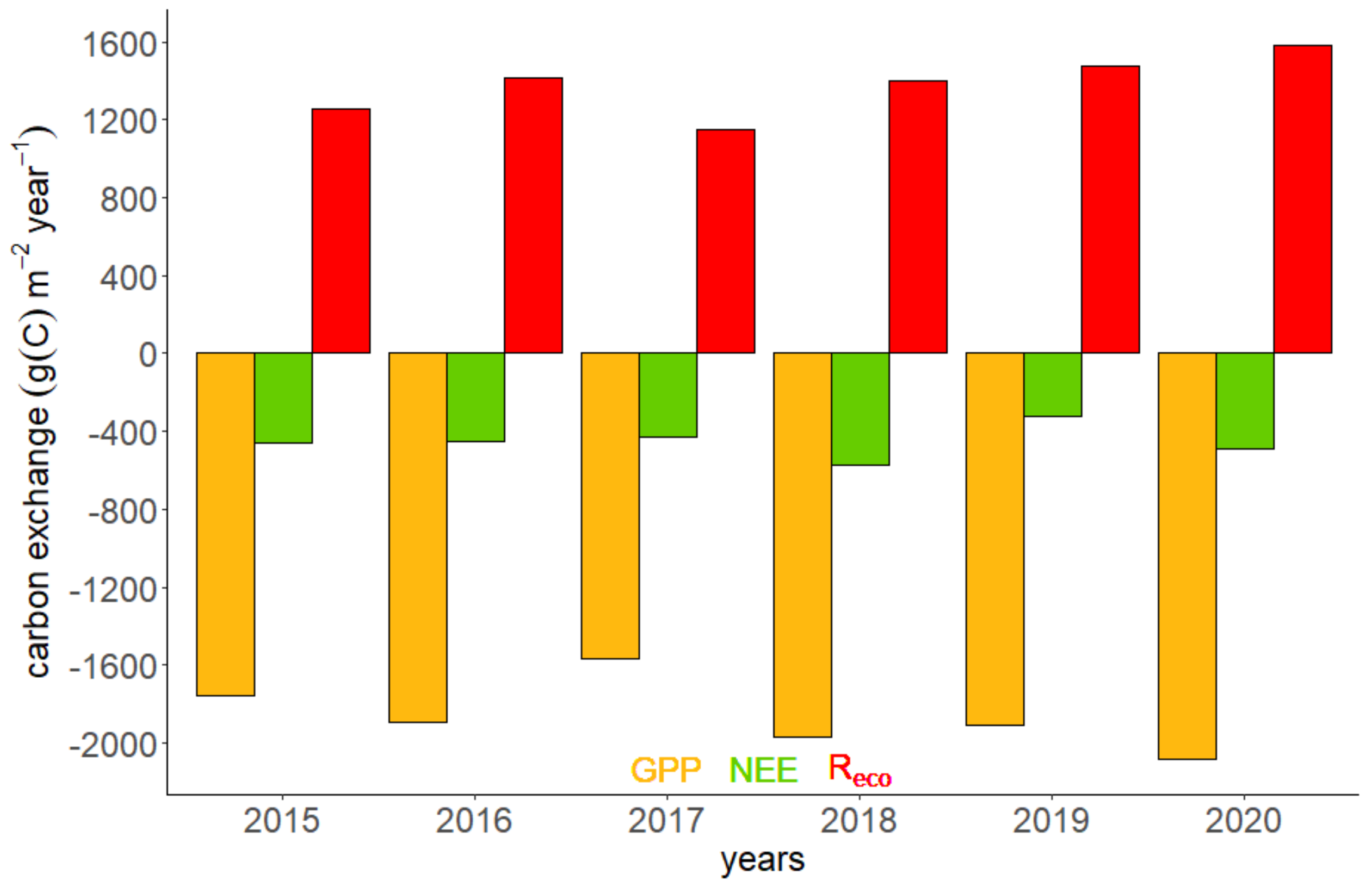
Substantial increase in NEE, in comparison with previous years, was observed during the year 2018. The studied forest showed the smallest NEE in 2019 and second, after 2020, highest annual Reco. During the measurement period, the year 2020 exhibited the highest GPP. In this year also, the highest annual Reco was observed (Figure 3).
3.3. Influence of Decoupling on above Canopy Derived Carbon Fluxes in the Study Years 2019–2020
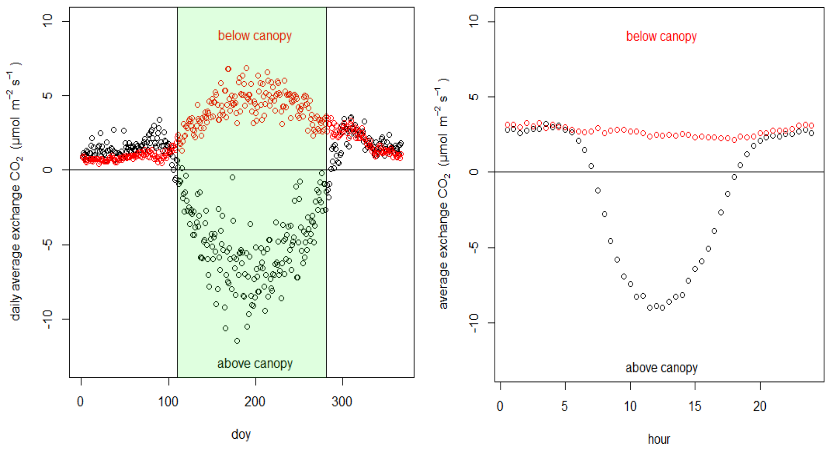
The patterns of above and below canopy fluxes were analyzed to determine how much of the below canopy fluxes are represented by the above canopy fluxes. On average, above canopy fluxes exhibit CUP for the days of the year 110–281 (Figure 4, on the left). At nights, often under conditions of very low or no turbulence when CO2 accumulates close to the ground, below canopy fluxes were slightly higher than above canopy fluxes (Figure 4, on the right).
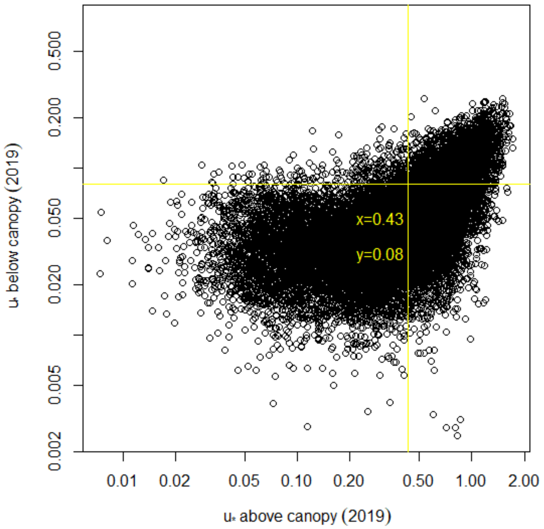
u* two-level filtering
For 2019, we derived the filtering thresholds of u* above the canopy 0.43 m s−1 and below the canopy 0.08 m s−1 (Figure 5). Periods with both u* above and below the canopy above their thresholds indicate full coupling, i.e., sufficient mixing across the whole canopy.
CO2 flux diurnal variation based on single- and two-level filtering
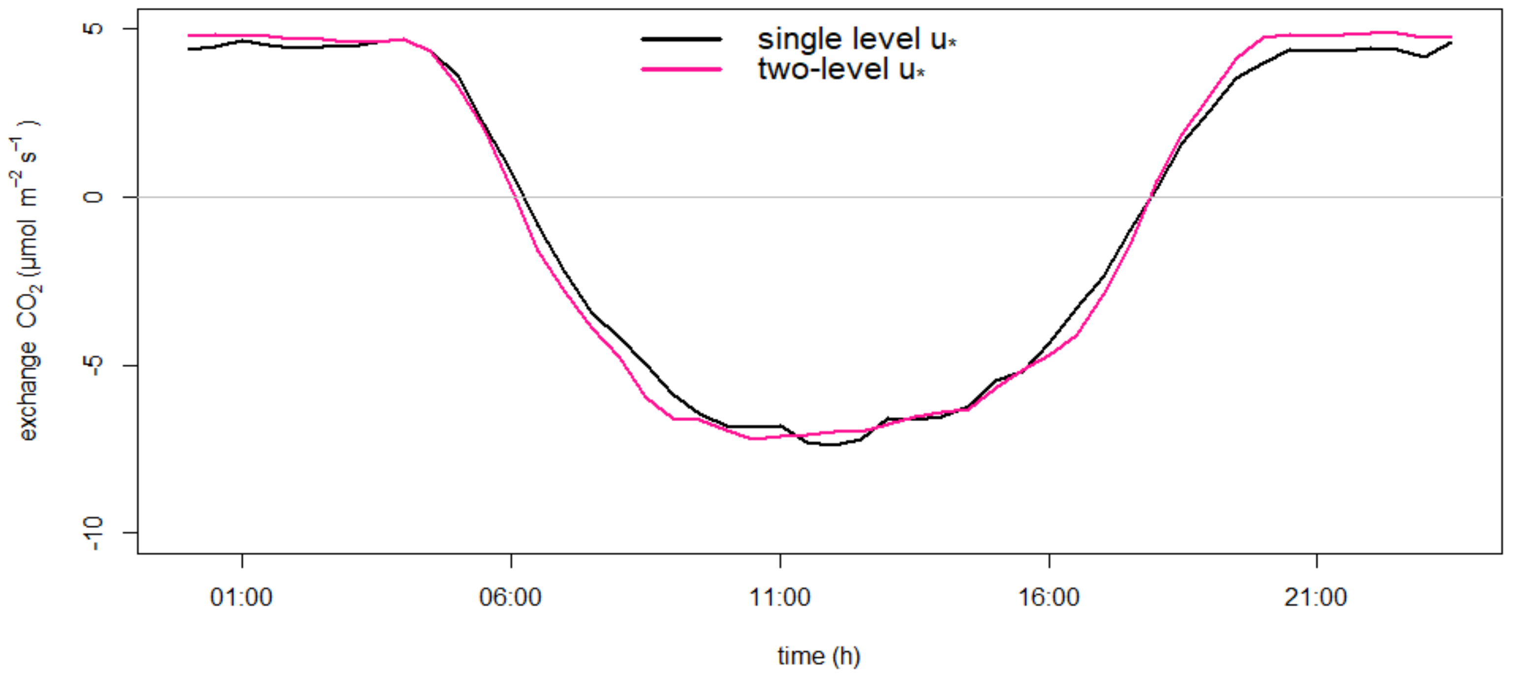
The mean diurnal variation of single- and two-level u* filtered CO2 exchange showed a typical behavior characterized by CO2 uptake from around 5:00 till about 19:00, on average, and CO2 emission only during the night hours. Small differences between the single- and two-level u* filtered data can be observed. The two-level filtered data indicate higher respiration during nighttime which depicts the effect of accounting for decoupling with the two-level filtering (Figure 6).
Sensitivity analysis of decoupling filtering thresholds
As the differences between the single- and two-level u* filtered data seemed only marginal, we conducted a sensitivity analysis of the additional below canopy u* filtering threshold. With this procedure, we wanted to evaluate how sensitive the above canopy derived annual C exchange is for the additional decoupling filtering (Table 2).
In the case that decoupling would significantly hinder the vertical CO2 transport from forest floor through canopy, the annual cumulative C results should become less negative with increasing strictness of decoupling filtering, as stricter filtering should better account for below canopy respiration. Our results, however, suggest that at the study site, decoupling occurs regularly, but has no significant effect on above canopy derived annual cumulative C exchange. The annual storage flux in the year 2019 equals 0.9 g m−2, thus, would not change this result.
4. Discussion
The highest NEE in 2018 in comparison to the other study years was generated by an exceptionally warm spring (with earlier leaf development) and a dry summer [9]. After this drought year, two years with high amounts of precipitation followed, which, in consequence, led to the highest GPP in 2020 (Figure 2 and Figure 3). However, wet conditions were also associated with high ecosystem respiration and the NEE in 2020 was the smallest among all studied years. Based on our results, we assume that this ecosystem was not characterized by reduced growth after the drought year 2018 and the so-called ”legacy effect” which is most dominant in dry ecosystems [53].
Analyzing the influence of decoupling on above canopy derived carbon fluxes, we observed positive below canopy fluxes over the whole course of the year (Figure 4, left). They indicate that decoupling outside of the CUP period would lead to an underestimation of the above canopy derived ecosystem respiration, and ignoring this phenomenon during the CUP period would yield an overestimation of the ecosystem carbon sink strength [54,55].
The u* two-level decoupling thresholds which we derived are comparable to other sites [20], though differences exhibit the threshold dependency on site-specific characteristics. On average, the two-level filtered data showed a higher respiration signal during nighttime than the single-level filtered data (Figure 6), which would confirm the theoretical assumption that the two-level filtered data are capturing more respiration signals from below canopy as they consider only fully coupled periods. On an annual scale, however, this does not make an impact on the carbon exchange at our site. There might also be filtering effects during daytime which lead to more negative (higher uptake) flux values during daytime periods (Figure 6) and counterbalance the nighttime effects of the two-level filtering. Furthermore, the study site is situated in very flat terrain which inhibits potential horizontal removal from CO2-rich below canopy air from the measurement volume. As a consequence, we observe no clear effect of the two-level filtering on the annual carbon exchange estimates (Table 2). At this specific site, contrary to a number of previous studies at other forest sites [20,21,22,32], the single-level u*filtering appears to be sufficient to address decoupling effects on annual carbon exchange values.
5. Summary and Conclusions
In this study, we evaluated different single- and two-level flux filtering strategies with regards to decoupling and its impact on above canopy derived CO2 fluxes. We hypothesized that conventional single-level EC flux filtering strategies like the u*filtering might not fully capture the forest CO2 exchange at the studied ecosystem. Concurrent below- and above-canopy EC measurements for the year 2019 showed the different carbon exchange dynamics of the respective layers well. While the whole canopy was a net carbon sink during spring and summer, the below canopy layer was a net source over the whole year. Though we observed regular and frequent decoupling of the below and above canopy air masses, we could not observe an effect of decoupling on the annual carbon exchange. We conclude that the exceptional flat terrain around our study site inhibits the removal of CO2-rich air from the measurement volume, consequently, a potentially biasing impact of decoupling on above canopy derived CO2 exchange on longer time scales.
Our study underlines the need of explicit decoupling investigations at each forest ecosystem, as decoupling is strongly site-specific, depending on canopy properties, vegetation structure, site meteorology and tower surrounding topography. Synthesis decoupling analyses of a multitude of forest sites around the globe can shed more light on the characteristics of decoupling in dependency of canopy properties, site meteorology and tower surrounding topography.
Author Contributions
Conceptualization: N.K. and G.J.; Methodology, N.K., G.J. and L.Š.; Software, N.K. and G.J.; Validation, N.K., G.J. and L.Š.; Formal Analysis: N.K. and G.J.; Investigation, N.K.; Resources, N.K. and G.J.; Data Curation, N.K. and G.J.; Writing—Original Draft Preparation, N.K.; Writing—Review and Editing, G.J., L.Š. and M.P.; Visualization, N.K., Supervision, M.P. All authors have read and agreed to the published version of the manuscript.
Funding
This research was funded by the Ministry of Education, Youth and Sports of the Czech Republic (CR) within the CzeCOS program, grant number LM2018123 and project SustES Adaptation strategies for sustainable ecosystem services and food security under adverse environmental conditions CZ.02.1.01/0.0/0.0/16_019/0000797.
Institutional Review Board Statement
Not applicable.
Informed Consent Statement
Not applicable.
Data Availability Statement
The data presented in this study are available on request from the corresponding author.
Acknowledgments
This work was supported by the Ministry of Education, Youth and Sports of CR within the CzeCOS program, grant number LM2018123. N.K and L.Š. acknowledge the support by the Ministry of Education, Youth and Sports of the Czech Republic for SustES—Adaptation strategies for sustainable ecosystem services and food security under adverse environmental conditions (CZ.02.1.01/0.0/0.0/16019/0000797).
Conflicts of Interest
The authors declare no conflict of interest.
References
- Schnitzler, A.; Hale, B.W.; Alsum, E. Biodiversity of floodplain forests in Europe and eastern North America: A comparative study of the Rhine and Mississippi Valleys. Biodivers. Conserv. 2005, 14, 97–117. [Google Scholar] [CrossRef]
- Ramsar Convention Secretariat. Ramsar Convention on Wetlands. Global Wetland Outlook: State of the World’s Wetlands and Their Services to People; Ramsar Convention Secretariat: Gland, Switzerland, 2018. [Google Scholar]
- Hanberry, B.B.; Kabrick, J.M.; He, H.S. Potential tree and soil carbon storage in a major historical floodplain forest with disrupted ecological function. Perspect. Plant Ecol. Evol. Syst. 2015, 17, 17–23. [Google Scholar] [CrossRef]
- Mitsch, W.J.; Bernal, B.; Nahlik, A.; Mander, Ü.; Zhang, L.; Anderson, C.J.; Jørgensen, S.E.; Brix, H. Wetlands, carbon, and climate change. Landsc. Ecol. 2013, 28, 583–597. [Google Scholar] [CrossRef]
- Joosten, H. Peatlands across the Globe. Chapter Two in Peatland Restoration and Ecosystem Services: Science, Policy and Practice; Cambridge University Press: Cambridge, UK, 2016. [Google Scholar]
- Moomaw, W.R.; Chmura, G.; Davies, G.T.; Finlayson, C.; Middleton, B.A.; Natali, S.M.; Perry, J.E.; Roulet, N.; Sutton-Grier, A. Wetlands in a Changing Climate: Science, Policy and Management. Wetlands 2018, 38, 183–205. [Google Scholar] [CrossRef] [Green Version]
- Mikac, S.; Žmegač, A.; Trlin, D.; Paulić, V.; Oršanić, M.; Anić, I. Drought-induced shift in tree response to climate in floodplain forests of Southeastern Europe. Sci. Rep. 2018, 8, 16495. [Google Scholar] [CrossRef]
- Heklau, H.; Jetschke, G.; Bruelheide, H.; Seidler, G.; Haider, S. Species-specific responses of wood growth to flooding and climate in floodplain forests in Central Germany. iForest—Biogeosci. For. 2019, 12, 226–236. [Google Scholar] [CrossRef]
- Kowalska, N.; Šigut, L.; Stojanović, M.; Fischer, M.; Kyselova, I.; Pavelka, M. Analysis of floodplain forest sensitivity to drought. Philos. Trans. R. Soc. B Biol. Sci. 2020, 375, 20190518. [Google Scholar] [CrossRef]
- Nezval, O.; Krejza, J.; Světlík, J.; Šigut, L.; Horáček, P. Comparison of traditional ground-based observations and digital remote sensing of phenological transitions in a floodplain forest. Agric. For. Meteorol. 2020, 291, 108079. [Google Scholar] [CrossRef]
- Salimi, S.; Almuktar, S.A.; Scholz, M. Impact of climate change on wetland ecosystems: A critical review of experimental wetlands. J. Environ. Manag. 2021, 286, 112160. [Google Scholar] [CrossRef]
- Valach, A.C.; Kasak, K.; Hemes, K.S.; Anthony, T.L.; Dronova, I.; Taddeo, S.; Silver, W.L.; Szutu, D.; Verfaillie, J.; Baldocchi, D.D. Productive wetlands restored for carbon sequestration quickly become net CO2 sinks with site-level factors driving uptake variability. PLoS ONE 2021, 16, e0248398. [Google Scholar] [CrossRef]
- Aubinet, M.; Vesala, T.; Papale, D. (Eds.) Eddy Covariance: A Practical Guide to Measurement and Data Analysis; Springer: Dordrecht, The Netherlands, 2012; 438p. [Google Scholar]
- Foken, T.; Aubinet, M.; Leuning, R. The Eddy Covariance Method. In Eddy Covariance; Springer Atmospheric Sciences; Aubinet, M., Vesala, T., Papale, D., Eds.; Springer: Dordrecht, The Netherlands, 2012. [Google Scholar] [CrossRef]
- Baldocchi, D.D. Assessing the eddy covariance technique for evaluating carbon dioxide exchange rates of ecosystems: Past, present and future. Glob. Chang. Biol. 2003, 9, 479–492. [Google Scholar] [CrossRef] [Green Version]
- Lasslop, G.; Reichstein, M.; Papale, D.; Richardson, A.D.; Arneth, A.; Barr, A.; Stoy, P.; Wohlfahrt, G. Separation of net ecosystem exchange into assimilation and respiration using a light response curve approach: Critical issues and global evaluation. Glob. Chang. Biol. 2010, 16, 187–208. [Google Scholar] [CrossRef] [Green Version]
- Aubinet, M.; Berbigier, P.; Bernhofer, C.; Cescatti, A.; Feigenwinter, C.; Granier, A.; Grünwald, T.; Havrankova, K.; Heinesch, B.; Longdoz, B.; et al. Comparing CO2 exchange and advection conditions at night at different carboeuroflux sites. Bound. Layer Metorol. 2005, 116, 63–93. [Google Scholar] [CrossRef] [Green Version]
- Acevedo, O.C.; Mahrt, L.; Puhales, F.S.; Costa, F.D.; Medeiros, L.E.; Degrazia, G.A. Contrasting structures between the decoupled and coupled states of the stable boundary layer. Q. J. R. Meteorol. Soc. 2016, 142, 693–702. [Google Scholar] [CrossRef]
- Alekseychik, P.; Mammarella, I.; Launiainen, S.; Rannik, Ü.; Vesala, T. Evolution of the nocturnal decoupled layer in a pine forest canopy. Agric. For. Meteorol. 2013, 174–175, 15–27. [Google Scholar] [CrossRef]
- Thomas, C.K.; Martin, J.G.; Law, B.; Davis, K. Toward biologically meaningful net carbon exchange estimates for tall, dense canopies: Multi-level eddy covariance observations and canopy coupling regimes in a mature Douglas-fir forest in Oregon. Agric. For. Meteorol. 2013, 173, 14–27. [Google Scholar] [CrossRef]
- Jocher, G.; Löfvenius, M.; De Simon, G.; Hörnlund, T.; Linder, S.; Lundmark, T.; Marshall, J.; Nilsson, M.B.; Näsholm, T.; Tarvainen, L.; et al. Apparent winter CO2 uptake by a boreal forest due to decoupling. Agric. For. Meteorol. 2017, 232, 23–34. [Google Scholar] [CrossRef]
- Jocher, G.; Fischer, M.; Šigut, L.; Pavelka, M.; Sedlák, P.; Katul, G. Assessing decoupling of above and below canopy air masses at a Norway spruce stand in complex terrain. Agric. For. Meteorol. 2020, 294, 108149. [Google Scholar] [CrossRef]
- Goulden, M.L.; Munger, J.W.; Fan, S.-M.; Daube, B.C.; Wofsy, S.C. Measurements of carbon sequestration by long-term eddy covariance: Methods and a critical evaluation of accuracy. Glob. Chang. Biol. 1996, 2, 169–182. [Google Scholar] [CrossRef] [Green Version]
- Aubinet, M.; Grelle, A.; Ibrom, A.; Rannik, U.; Moncrieff, J.; Foken, T.; Kowalski, A.S.; Martin, P.H.; Berbigier, P.; Bernhofer, C.; et al. Estimates of the annual net carbon and water exchange of forests: The EUROFLUX methodology. Adv. Ecol. Res. 1999, 30, 113–175. [Google Scholar] [CrossRef]
- Barr, A.; Morgenstern, K.; Black, T.; McCaughey, J.; Nesic, Z. Surface energy balance closure by the eddy-covariance method above three boreal forest stands and implications for the measurement of the CO2 flux. Agric. For. Meteorol. 2006, 140, 322–337. [Google Scholar] [CrossRef]
- Papale, D.; Reichstein, M.; Aubinet, M.; Canfora, E.; Bernhofer, C.; Kutsch, W.; Longdoz, B.; Rambal, S.; Valentini, R.; Vesala, T.; et al. Towards a standardized processing of Net Ecosystem Exchange measured with eddy covariance technique: Algorithms and uncertainty estimation. Biogeosciences 2006, 3, 571–583. [Google Scholar] [CrossRef] [Green Version]
- Pastorello, G.; Trotta, C.; Canfora, E.; Chu, H.; Christianson, D.; Cheah, Y.-W.; Poindexter, C.; Chen, J.; Elbashandy, A.; Humphrey, M.; et al. The FLUXNET2015 dataset and the ONEFlux processing pipeline for eddy covariance data. Sci. Data 2020, 7, 225. [Google Scholar] [CrossRef]
- Falge, E.; Baldocchi, D.; Olson, R.; Anthoni, P.; Aubinet, M.; Bernhofer, C.; Burba, G.; Ceulemans, R.; Clement, R.; Dolman, H.; et al. Gap filling strategies for defensible annual sums of net ecosystem exchange. Agric. Forest Meteorol. 2001, 107, 43–69. [Google Scholar] [CrossRef] [Green Version]
- Papale, D.; Valentini, R. A new assessment of European forests carbon exchanges by eddy fluxes and artificial neural network spatialization. Glob. Chang. Biol. 2003, 9, 525–535. [Google Scholar] [CrossRef]
- Reichstein, M.; Falge, E.; Baldocchi, D.; Papale, D.; Aubinet, M.; Berbigier, P.; Bernhofer, C.; Buchmann, N.; Gilmanov, T.; Granier, A.; et al. On the separation of net ecosystem exchange into assimilation and ecosystem respiration: Review and improved algorithm. Glob. Chang. Biol. 2005, 11, 1424–1439. [Google Scholar] [CrossRef]
- Paul-Limoges, E.; Wolf, S.; Eugster, W.; Hörtnagl, L.; Buchmann, N. Below-canopy contributions to ecosystem CO2 fluxes in a temperate mixed forest in Switzerland. Agric. For. Meteorol. 2017, 247, 582–596. [Google Scholar] [CrossRef] [Green Version]
- Jocher, G.; Marshall, J.; Nilsson, M.B.; Linder, S.; De Simon, G.; Hörnlund, T.; Lundmark, T.; Näsholm, T.; Löfvenius, M.O.; Tarvainen, L.; et al. Impact of Canopy Decoupling and Subcanopy Advection on the Annual Carbon Balance of a Boreal Scots Pine Forest as Derived from Eddy Covariance. J. Geophys. Res. Biogeosci. 2017, 123, 303–325. [Google Scholar] [CrossRef]
- Freundorfer, A.; Rehberg, I.; Law, B.E.; Thomas, C. Forest wind regimes and their implications on cross-canopy coupling. Agric. For. Meteorol. 2019, 279, 107696. [Google Scholar] [CrossRef]
- Speckman, H.N.; Frank, J.M.; Bradford, J.B.; Miles, B.L.; Massman, W.J.; Parton, W.J.; Ryan, M.G. Forest ecosystem respiration estimated from eddy covariance and chamber measurements under high turbulence and substantial tree mortality from bark beetles. Glob. Chang. Biol. 2014, 21, 708–721. [Google Scholar] [CrossRef]
- Thomas, C.; Foken, T. Flux contribution of coherent structures and its implications for the exchange of energy and matter in a tall spruce canopy. Bound.-Layer Meteorol. 2007, 123, 317–337. [Google Scholar] [CrossRef]
- Acosta, M.; Darenova, E.; Dušek, J.; Pavelka, M. Soil carbon dioxide fluxes in a mixed floodplain forest in the Czech Republic. Eur. J. Soil Biol. 2017, 82, 35–42. [Google Scholar] [CrossRef]
- Nicolini, G.; Sabbatini, S.; Papale, D. ICOS Ecosystem Instructions for Radiation Measurements (Version 20180620); ICOS Ecosystem Thematic Centre, DIBAF University of Tuscia: Viterbo, Italy, 2017. [Google Scholar] [CrossRef]
- Op de Beeck, M.; Sabbatini, S.; Papale, D. ICOS Ecosystem Instructions for Soil Meteorological Measurements (TS, SWC, G) (Version 20180615); ICOS Ecosystem Thematic Centre, DIBAF University of Tuscia: Viterbo, Italy, 2017. [Google Scholar] [CrossRef]
- Sabbatini, S.; Nicolini, G.; Op de Beeck, M.; Papale, D. ICOS Ecosystem Instructions for Air Meteorological Measure-ments (TA, RH, PA, WS, WD) (Version 20170130); ICOS Ecosystem Thematic Centre, DIBAF University of Tuscia: Viterbo, Italy, 2017. [Google Scholar] [CrossRef]
- Rebmann, C.; Aubinet, M.; Schmid, H.; Arriga, N.; Aurela, M.; Burba, G.; Clement, R.; De Ligne, A.; Fratini, G.; Gielen, B.; et al. ICOS eddy covariance flux-station site setup: A review. Int. Agrophys. 2018, 32, 471–494. [Google Scholar] [CrossRef]
- Vermeulen, A.; Hellström, M.; Mirzov, O.; Karstens, U.; D’Onofrio, C.; Lankreijer, H. The ICOS Carbon Portal as an example of a FAIR community data repository supporting scientific workflows. In Proceedings of the EGU General Assembly 2021, Online, 19–30 April 2021. EGU21-8458. [Google Scholar] [CrossRef]
- Lee, X.; Massmann, W.J.; Law, B. (Eds.) Handbook of Micrometeorology: A Guide for Surface Flux Measurements and Analysis; Kluwer: New York, NY, USA, 2004; 250p. [Google Scholar]
- Wilczak, J.M.; Oncley, S.P.; Stage, S.A. Sonic Anemometer Tilt Correction Algorithms. Bound.-Layer Meteorol. 2001, 99, 127–150. [Google Scholar] [CrossRef]
- Moore, C.J. Frequency response corrections for eddy correlation systems. Bound.-Layer Meteorol. 1986, 37, 17–35. [Google Scholar] [CrossRef]
- Schotanus, P.; Nieuwstadt, F.T.; De Bruin, H.A. Temperature measurement with a sonic anemometer and its application to heat and moisture fluctuations. Bound.-Layer Meteorol. 1983, 26, 81–93. [Google Scholar] [CrossRef]
- Foken, T.; Göckede, M.; Mauder, M.; Mahrt, L.; Amiro, B.D.; Munger, W.J. Post-field data quality control. In Handbook of micrometeorology: A guide for surface flux measurements and analysis; Lee, X., Massmann, W.J., Law, B., Eds.; Kluwer: New York, NY, USA, 2004; pp. 181–208. [Google Scholar]
- R Core Team. A Language and Environment for Statistical Computing; R Foundation for Statistical Computing: Vienna, Austria, 2017. [Google Scholar]
- Wutzler, T.; Reichstein, M.; Moffat, A.M.; Menzer, O.; Migliavacca, M.; Sickel, K.; Šigut, L. Post Processing of (Half)Hourly Eddy Covariance Measurements; R Package Version 1.1.5; R Foundation for Statistical Computing: Vienna, Austria, 2018. [Google Scholar]
- Wohlfahrt, G.; Galvagno, M. Revisiting the choice of the driving temperature for eddy covariance CO2 flux partitioning. Agric. For. Meteorol. 2017, 237–238, 135–142. [Google Scholar] [CrossRef]
- Aubinet, M.; Chermanne, B.; Vandenhaute, M.; Longdoz, B.; Yernaux, M.; Laitat, E. Long term carbon dioxide exchange above a mixed forest in the Belgian Ardennes. Agric. For. Meteorol. 2001, 108, 293–315. [Google Scholar] [CrossRef]
- Nicolini, G.; Aubinet, M.; Feigenwinter, C.; Heinesch, B.; Lindroth, A.; Mamadou, O.; Moderow, U.; Mölder, M.; Montagnani, L.; Rebmann, C.; et al. Impact of CO2 storage flux sampling uncertainty on net ecosystem exchange measured by eddy covariance. Agric. For. Meteorol. 2018, 248, 228–239. [Google Scholar] [CrossRef] [Green Version]
- Toreti, A.; Belward, A.; Perez-Dominguez, I.; Naumann, G.; Luterbacher, J.; Cronie, O.; Seguini, L.; Manfron, G.; Lopez-Lozano, R.; Baruth, B.; et al. The Exceptional 2018 European Water Seesaw Calls for Action on Adaptation. Earth Futur. 2019, 7, 652–663. [Google Scholar] [CrossRef]
- Anderegg, W.R.L.; Schwalm, C.R.; Biondi, F.; Camarero, J.J.; Koch, G.W.; Litvak, M.; Ogle, K.; Shaw, J.D.; Shevliakova, E.; Williams, P.; et al. Pervasive drought legacies in forest ecosystems and their implications for carbon cycle models. Science 2015, 349, 528–532. [Google Scholar] [CrossRef] [Green Version]
- McHugh, I.D.; Beringer, J.; Cunningham, S.C.; Baker, P.J.; Cavagnaro, T.R.; Mac Nally, R.; Thompson, R.M. Interactions between nocturnal turbulent flux, storage and advection at an “ideal” eucalypt woodland site. Biogeosciences 2017, 14, 3027–3050. [Google Scholar] [CrossRef] [Green Version]
- Feigenwinter, C.; Bernhofer, C.; Eichelmann, U.; Heinesch, B.; Hertel, M.; Janous, D.; Kolle, O.; Lagergren, F.; Lindroth, A.; Minerbi, S.; et al. Comparison of horizontal and vertical advective CO2 fluxes at three forest sites. Agric. For. Meteorol. 2008, 148, 12–24. [Google Scholar] [CrossRef]
Figure 1.
Map of Czech Republic (left), the study site Lanžhot with the location of the EC tower (middle) and the view of the floodplain forest ecosystem from above (right).
Figure 1.
Map of Czech Republic (left), the study site Lanžhot with the location of the EC tower (middle) and the view of the floodplain forest ecosystem from above (right).

Figure 2.
Time series of daily mean air temperature (Tair), soil temperature (Tsoil) and daily sums of precipitation (P) over the whole study period at the study site Lanžhot, Czech Republic. The lines in the uppermost two panels indicate local polynomial regression fittings (loess; span = 0.1).
Figure 2.
Time series of daily mean air temperature (Tair), soil temperature (Tsoil) and daily sums of precipitation (P) over the whole study period at the study site Lanžhot, Czech Republic. The lines in the uppermost two panels indicate local polynomial regression fittings (loess; span = 0.1).

Figure 3.
Annual totals of gross primary production (GPP), net ecosystem exchange (NEE) and ecosystem respiration (Reco) for the measurement period 2015–2020 at the floodplain forest in Lanžhot, Czech Republic.
Figure 3.
Annual totals of gross primary production (GPP), net ecosystem exchange (NEE) and ecosystem respiration (Reco) for the measurement period 2015–2020 at the floodplain forest in Lanžhot, Czech Republic.

Figure 4.
Daily average exchange of CO2 above and below the canopy during the years 2019–2020 (on the left) and averaged diurnal patterns covering the years 2019–2020 (on the right).
Figure 4.
Daily average exchange of CO2 above and below the canopy during the years 2019–2020 (on the left) and averaged diurnal patterns covering the years 2019–2020 (on the right).

Figure 5.
Relation between below canopy u* vs. above canopy u* (black circles; 30 min resolution; m s−1; both axes are in logarithmic scale). The yellow vertical and horizontal line indicate the estimated above and below the canopy u* thresholds, respectively, which distinguish weak turbulent periods from the period when the canopy layers were fully coupled.

Figure 6.
Mean diurnal variation of CO2 exchange (NEE) based on single- and two-level u* filtered data for the year 2019.
Figure 6.
Mean diurnal variation of CO2 exchange (NEE) based on single- and two-level u* filtered data for the year 2019.


Table 1.
Overview over the used instrumentation in the course of this study.
| Site Name: Lanžhot | Sensor | Height/Depth (m) |
|---|---|---|
| Eddy covariance | LI-7200RS, LI-COR, Inc. (NE, USA), HS-50, (Gill Instruments, UK) | 44 m until 22 October 2018, later 48 m |
| Global incoming radiation (GR) | CNR4 (Kipp & Zonen, Delft, The Netherlands) | 42 m until 22 October 2018, later 44 m |
| Air temperature (Tair) and relative humidity (RH) | EMS 33 (EMS Brno, Czech Republic) until 21 June 2019, later HMP 155 (Vaisala, Vantaa, Finland), HMP 155 (Vaisala, Vantaa, Finland), | 35 m |
| Soil temperature (Tsoil) | Pt100 (Sensit, CZ) | 0.02 m |
| Precipitation (P) | Laser Precipitation monitor, Thies Clima (Göttingen, Germany) | 44 m until 22 October 2018, later 48 m |
Table 2.
Sensitivity analysis for u*b and its influence on the carbon exchange values for 2019.
| u* above the Canopy (u*a) | u* below the Canopy (u*b) | C Exchange (g m−2) for the 2019 Year | Percentage of Gaps after Two-Level u* Filtering in Relation to Single Level u* Filtering (%) |
|---|---|---|---|
| u*a = 0.43 | – | −188.9 | – |
| u*a = 0.43 | u*b = 0.02 | −185.5 | 1.6 |
| u*a = 0.43 | u*b = 0.03 | −181.3 | 6.0 |
| u*a = 0.43 | u*b = 0.04 | −216.8 | 11.9 |
| u*a = 0.43 | u*b = 0.05 | −201.0 | 18.0 |
| u*a = 0.43 | u*b = 0.06 | −209.0 | 23.5 |
| u*a = 0.43 | u*b = 0.07 | −203.7 | 27.8 |
| u*a = 0.43 | u*b = 0.08 | −192.6 | 31.0 |
Publisher’s Note: MDPI stays neutral with regard to jurisdictional claims in published maps and institutional affiliations. |
© 2022 by the authors. Licensee MDPI, Basel, Switzerland. This article is an open access article distributed under the terms and conditions of the Creative Commons Attribution (CC BY) license (https://creativecommons.org/licenses/by/4.0/).
Share and Cite
MDPI and ACS Style
Kowalska, N.; Jocher, G.; Šigut, L.; Pavelka, M. Does Below-Above Canopy Air Mass Decoupling Impact Temperate Floodplain Forest CO2 Exchange? Atmosphere 2022, 13, 437. https://doi.org/10.3390/atmos13030437
AMA Style
Kowalska N, Jocher G, Šigut L, Pavelka M. Does Below-Above Canopy Air Mass Decoupling Impact Temperate Floodplain Forest CO2 Exchange? Atmosphere. 2022; 13(3):437. https://doi.org/10.3390/atmos13030437
Chicago/Turabian StyleKowalska, Natalia, Georg Jocher, Ladislav Šigut, and Marian Pavelka. 2022. "Does Below-Above Canopy Air Mass Decoupling Impact Temperate Floodplain Forest CO2 Exchange?" Atmosphere 13, no. 3: 437. https://doi.org/10.3390/atmos13030437
Note that from the first issue of 2016, this journal uses article numbers instead of page numbers. See further details here.