Article

Determination of PM1 Sources at a Prague Background Site during the 2012–2013 Period Using PMF Analysis of Combined Aerosol Mass Spectra

1
Department of Aerosol Chemistry and Physics, Institute of Chemical Process Fundamentals, Czech Academy of Sciences, Rozvojová 2/135, 165 02 Prague, Czech Republic
2
Faculty of Science, Institute for Environmental Studies, Charles University in Prague, Benátská 2, 128 01 Prague, Czech Republic
3
Department of Biomedical Engineering and Environmental Sciences, National Tsing Hua University, Hsinchu 30013, Taiwan
*
Authors to whom correspondence should be addressed.
Current Address: Mobile Source Laboratory Division, California Air Resources Board, Riverside, CA 92507, USA.
Atmosphere 2022, 13(1), 20; https://doi.org/10.3390/atmos13010020
Submission received: 1 November 2021 / Revised: 13 December 2021 / Accepted: 17 December 2021 / Published: 24 December 2021

Abstract

:
Two intensive measurement campaigns using a compact time-of-flight aerosol mass spectrometer were carried out at the suburban site in Prague (Czech Republic) in summer (2012) and winter (2013). The aim was to determine the aerosol sources of the NR-PM1 fraction by PMF analysis of organic (OA) and inorganic aerosol mass spectra. Firstly, an analysis of the OA mass spectra was performed. Hydrocarbon-like OA (HOA), biomass burning OA (BBOA), and two types of oxygenated OA (OOA1) and (OOA2) were identified in summer. In winter, HOA, BBOA, long-range oxygenated OA (LROOA), and local oxygenated OA (LOOA) were determined. The identified HOA and BBOA factors were then used as additional input for the subsequent ME-2 analysis of the combined organic and inorganic spectra. This analysis resulted in six factors in both seasons. All of the previously reported organic factors were reidentified and expanded with the inorganic part of the spectra in both seasons. Two predominantly inorganic factors ammonium sulphate (AMOS) and ammonium nitrate (AMON) were newly identified in both seasons. Despite very similar organic parts of the mass profiles, the daily cycles of HOA and LOOA differed significantly in winter. It appears that the addition of the inorganic part of the mass profile, in some cases, reduces the ability of the model to identify physically meaningful factors.

1. Introduction

Atmospheric aerosol (AA), the suspension of fine solid or liquid particles in the air, is an important area of research due to its effect on climate [1,2], visibility [3], hydrological cycle [4,5], and also for its harmful effect on human health [6,7]. Atmospheric aerosol is a complex mixture of organic and inorganic compounds. Organic aerosols (OAs) are still poorly described for thousands of compounds originating from various anthropogenic and natural sources. The evolution of OAs in the atmosphere is also very complicated and still partly unclear. Primary organic aerosols (POAs), originating mostly from combustion, are aging in the atmosphere, forming part of the secondary OA (SOA) through physical and chemical processes such as oxidation, nucleation, and condensation [8]. An additional part of SOA is formed by a chemical reaction from various organic gaseous precursors both of natural and anthropogenic origin. Although the inorganic part of the aerosol matter is better explored due to a smaller number of chemical species and less complex chemistry, it is important to include inorganic aerosol (IA) if we want to perform a comprehensive analysis of aerosol sources influencing the measurement site because IA represents from 10 to 80% of total submicron aerosol mass [9]. Understanding how aerosol is produced and evolved in the atmosphere is an essential step in defining strategies to reduce aerosol concentrations in the atmosphere.
Since there are thousands of specific compounds in the atmosphere, it seems reasonable to classify the particles into categories. Aerosol mass spectrometer (AMS) has proved to be a suitable instrument for this task. AMS is capable of measuring online the PM1 non-refractory aerosol mass concentrations and chemically speciated mass size distributions [10,11]. Moreover, due to very high time resolution from seconds to minutes [12], the AMS is suitable for measuring the aging of AA. A critical step of the analysis is to apportion AA spectra to sources and quantify the contribution of each source. This could be achieved by a variety of receptor modelling techniques. For example, the molecular marker-based chemical mass balance (CMB) approach is favourable for primary sources when we know their chemical profiles [13], but it is not suitable for identifying aerosol sources that have undergone a chemical transformation in the atmosphere. Principal component analysis (PCA) [14] allows us to model data without knowing the chemical composition of individual mass profiles but allows results containing negative values. In other words, PCA is not suitable for this type of task because it would allow negative concentrations, which is physically impossible. The analysis that meets the requirement of nonnegativity is positive matrix factorization (PMF) [15,16]. PMF is an example of a bilinear model that resolves the data matrix into ‘factors’ that contain the species that correlate in time; therefore, they have a common history, way of the origin, or chemical composition [17,18,19]. In recent years, a number of AMS data studies have been developed in Western Europe using a method based on PMF analysis [20,21,22,23]. Some studies have also been conducted in the Central European region [24,25], but in the Czech Republic, only analyses based on offline data from filter measurements from Prague [26] and the hot spot Ostrava region [27,28] have been reported so far.
This paper presents the results of the assessment of atmospheric aerosol sources determined on the principle of receptor modelling, using factor analysis. It analyses and compares concentrations and chemical profiles of sources from the measurement site on the outskirts of Prague in the Czech Republic obtained during the winter and summer seasons. The aim of the study was to extend the description of aerosol sources to include an inorganic part of spectra in order to obtain more comprehensive information on the size of AA sources and their chemical composition. By comparing the results of the analysis of the combined spectra with the organic spectra, we can then verify the stability and reliability of the results of the analysis of the combined spectra.

2. Materials and Methods

2.1. Measurement Site

The Prague-Suchdol site is located at the northwestern outskirts of Prague (Czech Republic; 50°7′36.473″ N, 14°23′5.513″ E, 277 m ASL). The newest part of the residential area is directly adjacent to the measurement station. The nearest older development is located about 500 m to the NW. A road with local traffic of about 15,000 cars per day is located at a distance of 200 m from the station. Roads with heavy traffic are not closer than three kilometres. A more detailed description of the measurement site in terms of aerosol chemical composition can be found elsewhere [29,30,31,32].
The Automated Imission Monitoring (AIM) station is located at the site that belongs to the Czech Hydrometeorological Institute (CHMI). The AIM provided us with data on the state of the atmosphere (e.g., wind speed, wind direction, temperature) and the concentrations of selected gaseous pollutants (SO2, NOx, CO, O3, Benzene, Toluene).

2.2. Instrumentation and Sampling

Two intensive measurement campaigns were performed at the urban background site Prague-Suchdol. The first measurement was conducted during summer 2012 (20.6.–1.8.), and the second campaign was performed in winter 2013 (9.1.–19.2.). Sampling was conducted with a PM2.5 size-selective inlet at a flow rate of 16.7 lpm. A stainless steel tube (3.3 m) with an inner diameter of 12 mm and isokinetic subsampling with a 3.18 mm stainless steel tube (0.1 m) was connected to a Nafion dryer (0.7 m), followed by a 3.18 mm copper tube linked to the AMS inlet. At the end of the main tubing, a vacuum pump with 16.7 lpm was installed to sustain the flow through the inlet and shorten the residence time of particles during sampling.
The measurement of aerosol particles was conducted via a compact time-of-flight aerosol mass spectrometer (C-ToF-AMS, Aerodyne, MA, USA; 1 min time resolution). The AMS measures the chemical and size-resolved composition of non-refractory (NR) aerosol particles up to 1 µm. For NR we refer to particles that vaporise at 600 °C at 1.3 × 10⁻³ Pa pressure. A detailed description of this instrument can be found in Drewnick et al. (2005) [33]. More details about the instrument operation and basic data can be found in Kubelová et al. (2015) [31].
Black carbon (BC) concentrations were calculated as equivalent black carbon [34] from a field semi-continuous OC/EC analyser (Sunset Laboratories) with a 2 h time resolution. More information about the EC/OC measurement is available in Vodička et al. (2013) [29]. During both campaigns, PM1 filter measurement with 24 h resolution took place at the station. Filter samples were analysed by ion chromatography; more details are given in Kubelová et al. (2015) [31]. Levoglucosan concentrations were obtained by using the HPAEC-PAD method at the National Tsing Hua University, Taiwan, according to Zhang et al. (2013) [35]. The concentrations of polycyclic aromatic hydrocarbons (PAHs) were measured directly by AMS [36].

2.2.1. Data Preparation

The collection efficiency (CE) was determined for each campaign by correlating sulphates measured by AMS with PM1 filter measurement of sulphate described in Kubelová et al. (2015) [31]. During the summer campaign, a CE of 0.29 was calculated, and a CE of 0.35 was calculated in winter. For more details on determining CE for each campaign, see Kubelová et al. (2015) [31].
Figure 1b shows that a period of very low concentrations starts on 30 June and lasts for about a week. Data measured in this range have a high noise contribution to the measured signal and, therefore, have been removed from the subsequent analysis.
After the time series were cleaned of outliers, input matrices of individual m/z concentrations over time for organics, sulphate, nitrate, ammonium, chloride, and potassium at 30 min time resolution were obtained directly from TOF-AMS Analysis Toolkit 1.53 (Squirrel, available at http://cires1.colorado.edu/jimenez-group/ToFAMSResources/ToFSoftware/, accessed on 10 December 2021). These matrices were used to create one large matrix including all organic and inorganic m/z. For organics, masses up to m/z number 160 were used. As some of the masses in the fragmentation table are calculated as fractions of other masses and, thus, do not contribute any additional variability to the PMF calculation, these calculated masses were excluded from further processing. Only the m/z 48 (SO+), 64 (SO2+), 80 (SO3+), 81 (HSO3+), 98 (H2SO4+) were used for sulphate; m/z 30 (NO+), 46 (NO2+) for nitrate; m/z 16 (NH2+), 17 (NH3+) for ammonium ion; m/z 35 (Cl+), 36 (HCl+) for chloride; m/z 39 (K+) for potassium. The size of the resulting matrix was 1942 × 145 for summer and 1991 × 285 for winter. Along with these, a minimal error vector was generated by Squirrel. This data set was then used as input to the SoFi engine.

2.3. Data Analysis

Analysis of C-ToF AMS mass spectra time series was performed by the source apportionment approach. Data were processed with a Multilinear Engine (ME-2) [37,38,39] which is capable to solve the PMF algorithm via the interface SoFi [40].
The most simple case of a multilinear engine is the bilinear model, where the unknowns constitute two groups [16,41]
x i , j = p = 1 P g i , p f p , j + e i , j
where the matrix x consists of measured values and the matrices g , f and e represent factor profile, time series, and residuals not fitted by the model, respectively. Then, P is defined as a number of factors. For ME-2 are the inputs g i , p and f p , j restricted for non-negative values only. ME-2 algorithm solves Equation (1) by the object function Q , which minimises the sum of the errors using the least-square algorithm.
Q = i = 1 m j = 1 n ( e i , j σ i , j ) 2
where σ i , j are the estimated measurement uncertainties calculated according to [42]. The monitored value is then the ratio Q / Q e x p , where Q e x p denotes the expected value of Q , which is a function of the size of the input data matrix.
A weakness of this approach could be that the calculated solution is not unique. That means we can obtain an infinite number of solutions due to rotational ambiguity [43]. This effect can be partially regulated by using the a-value (a-val) approach. The principle of this method is to input the a priori information about a part of the desired solution. The principle of this approach is described in Canonaco et al. (2013) [18] as
g j ,   s o l u t i o n = g j ± a . g j f i ,   s o l u t i o n = f j ± a . f j
where g j ,   s o l u t i o n and f i ,   s o l u t i o n are allowed to vary from g j and f i input by value a that can take values between 0 and 1.
All the measured data were analysed by the SoFi toolkit [18,40], (software version SoFi Pro 8.0.3.1), which utilises the ME-2 algorithm. All the calculations were run in ‘robust mode’ [16], with a threshold value = 4. For all the x i , j values a minimum error, smoothing was applied according to Ulbrich et al. (2009) [44]. The contribution of variables with a signal-to-noise ratio (SNR) in the range of 0.2–2 was down-weighted by a factor of 2. Variables with SNR < 0.2 were down-weighted 10 times. SNR ratio was defined in Paatero and Hopke (2003) [45] as
S N R =   x i , j 2 /   σ i , j 2
where x is signal and σ is estimated measurement uncertainties.
In all modelled cases, there was a problem with the stability of the solution for the combined AMS spectra, which is the most likely due to several inorganic species with high contributions causing solution bias. Therefore, first, an unanchored PMF run was performed only at organic aerosol data without fixing factors according to the guideline in Crippa et al. (2014) [22]. After obtaining a meaningful solution, the analysis of combined spectra, which are described in Section 2.2.1, was executed. As mentioned above, the initial results for combined spectra have a problem with the convergence of the solution. For the solution improvement, the a-value approach was utilised. Firstly, the HOA factor was fixed using the factor profile from the UMR AMS spectra database [46] (available at http://cires1.colorado.edu/jimenez-group/AMSsd/, accessed on 10 December 2021) with a-val ranging from 0.1 to 0.3. This did not lead to a satisfactory result, so the factors identified during the PMF analysis of the organic part of the data were used as the anchors. The best result was achieved when the HOA was fixed with the a-val = 0.15, and the BBOA also with the a-val = 0.15.
The factor identification was based on typical markers of factor profiles [47,48,49,50]. The final solution was chosen based on several criteria according to Crippa et al. (2013) [51]. The following analyses were performed: (1) Interpretation of mass spectra profiles and comparison with unit mass resolution (UMR) spectra from UMR AMS spectra database (available at http://cires1.colorado.edu/jimenez-group/AMSsd/, accessed on 10 December 2021), (2) temporal correlation with collocated measurements, and (3) physically and chemically meaningful shape of diurnal patterns. Although one of the analyses was performed on combined mass spectra, all data were measured by the same instrument, and therefore, no further correction due to the different error rates of the data was needed.

3. Results and Discussion

During the summer campaign, the prevailing wind was from the SW and W directions. The highest wind speeds were measured during both campaigns from the SW and NE directions (Figure S1a,c in the Supplementary Information, SI). However, the highest aerosol concentrations came from the SE direction, where most of the metropolitan area is located (Figure S1b). During the winter campaign, the most frequent winds were from the NW and W directions (Figure S1a). The highest PM1 concentrations were recorded from the W, NW, and N directions (Figure S1d). This may be explained by the existence of a residential area adjacent to the measuring stations, where some of the houses are heated with coal or wood boilers [52].

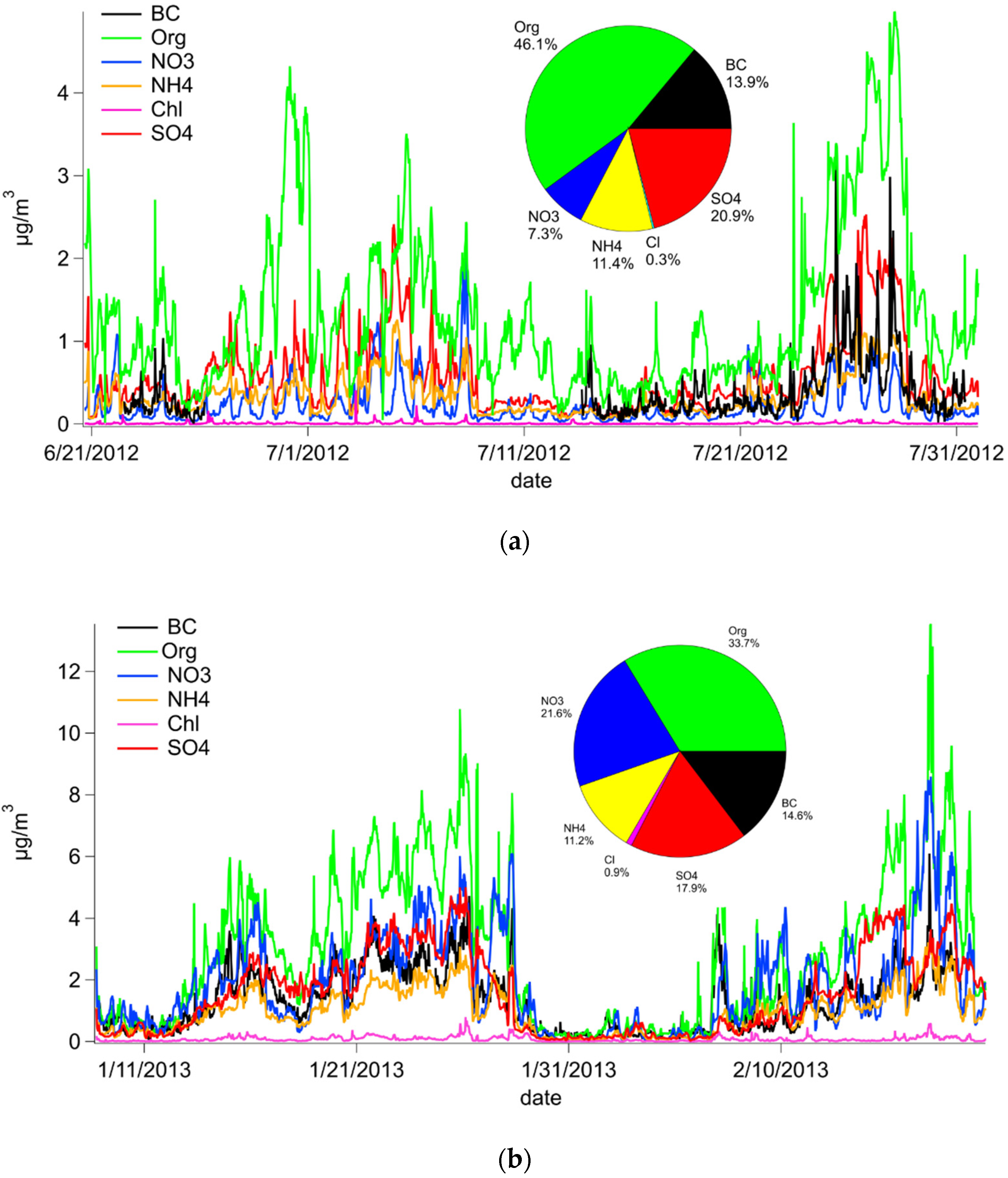
3.1. PM1 Chemical Composition

First, the results of the chemical composition, which were previously presented in Kubelová et al. (2015) [31] are summarised shortly. During the summer season, total PM1 concentrations ranged from 2 to 12 µg. Figure 1a shows that organic species (Org) accounted for 46% of the mass, while sulphate ions (SO42−) formed 21% of the mass, ammonium ions (NH4+), originating mainly from ammonium nitrate and ammonium sulphate, [8] accounted for about 11 % of the total mass, and nitrate (NO3) represented 7% of the mass. The amount of chloride (Cl) fluctuated around the detection limit for most of the campaign and represented about 0.3% of the total mass. These results are consistent with data measured at this station during other campaigns [53,54]. The amount of BC measured was almost 14%. Due to the prolonged outage of the OC/EC analyser during the campaign, mass fractions were only calculated for the period when the OC/EC was operational.
During the winter measurement campaign, total PM1 concentrations ranged from 2 to 70 µg, which in total represents a more than fivefold increase in maximum concentrations, compared with the summer season. In Figure 1b, we can see that the relative abundance of Org dropped below 34%, compared with summer, SO42− dropped to 18%, and NH4+ remained almost unchanged, at 12%. The proportion of NO3 increased significantly to 23%, which may be due to the higher stability of nitrate particles at low temperatures [55]. The proportion of Cl increased to 1%, which is due to three factors. One is the higher sea salt transport, and its transformation releasing HCl in the atmosphere in winter [56], use of gritting salt on nearby roads, and the other is coal combustion in local stoves [57]. The proportion of BC has increased to 14.6%, which is consistent with other measurements at the site [29,58] and with measurements at other stations of the same type [22,59]. Periods with higher aerosol concentrations are associated with a smaller boundary layer thickness [31] in which the aerosol cannot be diluted.
Figure 1a,b also show a more pronounced diurnal variation in concentrations during the summer season, with a significant decrease in afternoon concentrations, compared with night-time levels. This is mainly caused by intense thermal convective mixing and the supply of cleaner air from the upper atmosphere and the thermal decomposition of ammonium nitrate due to high temperatures during day time.

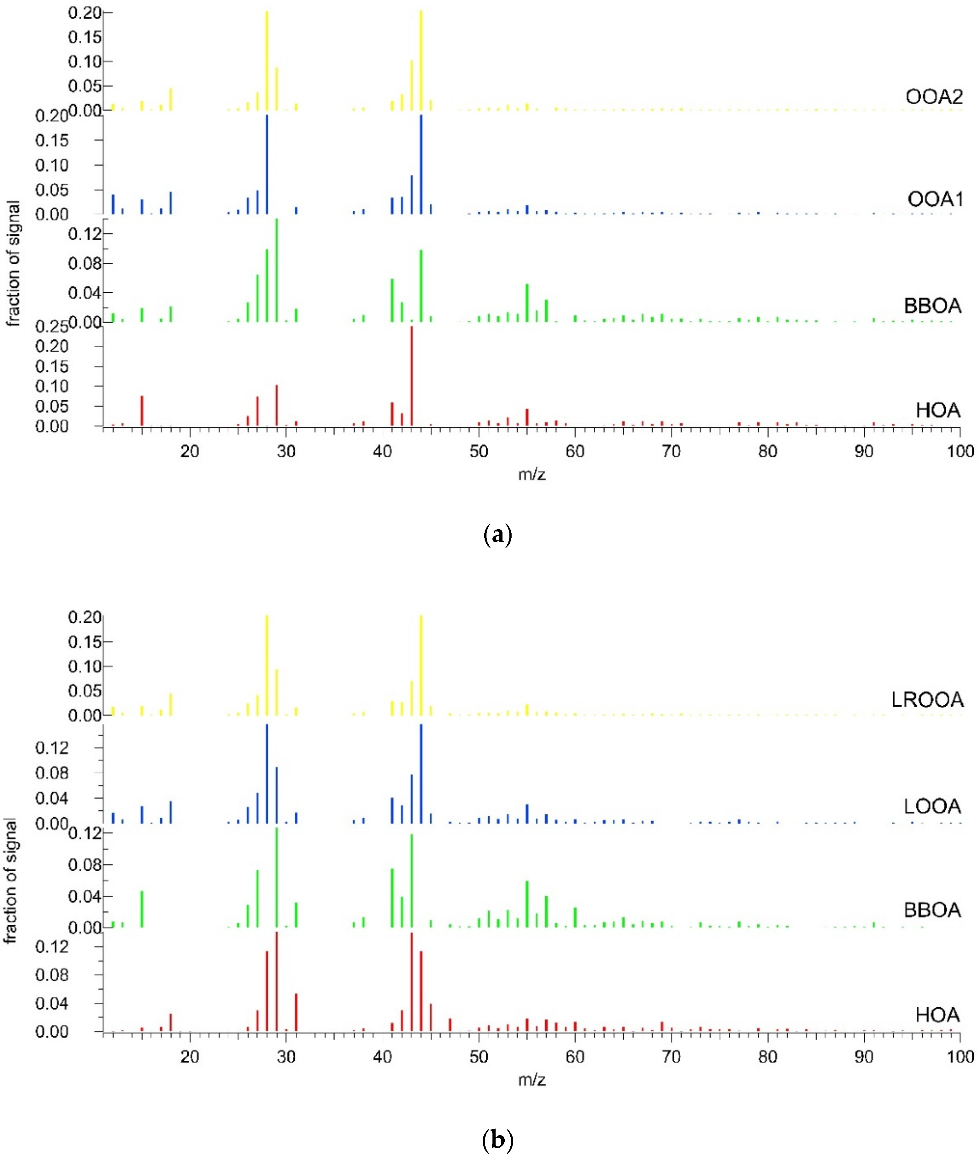
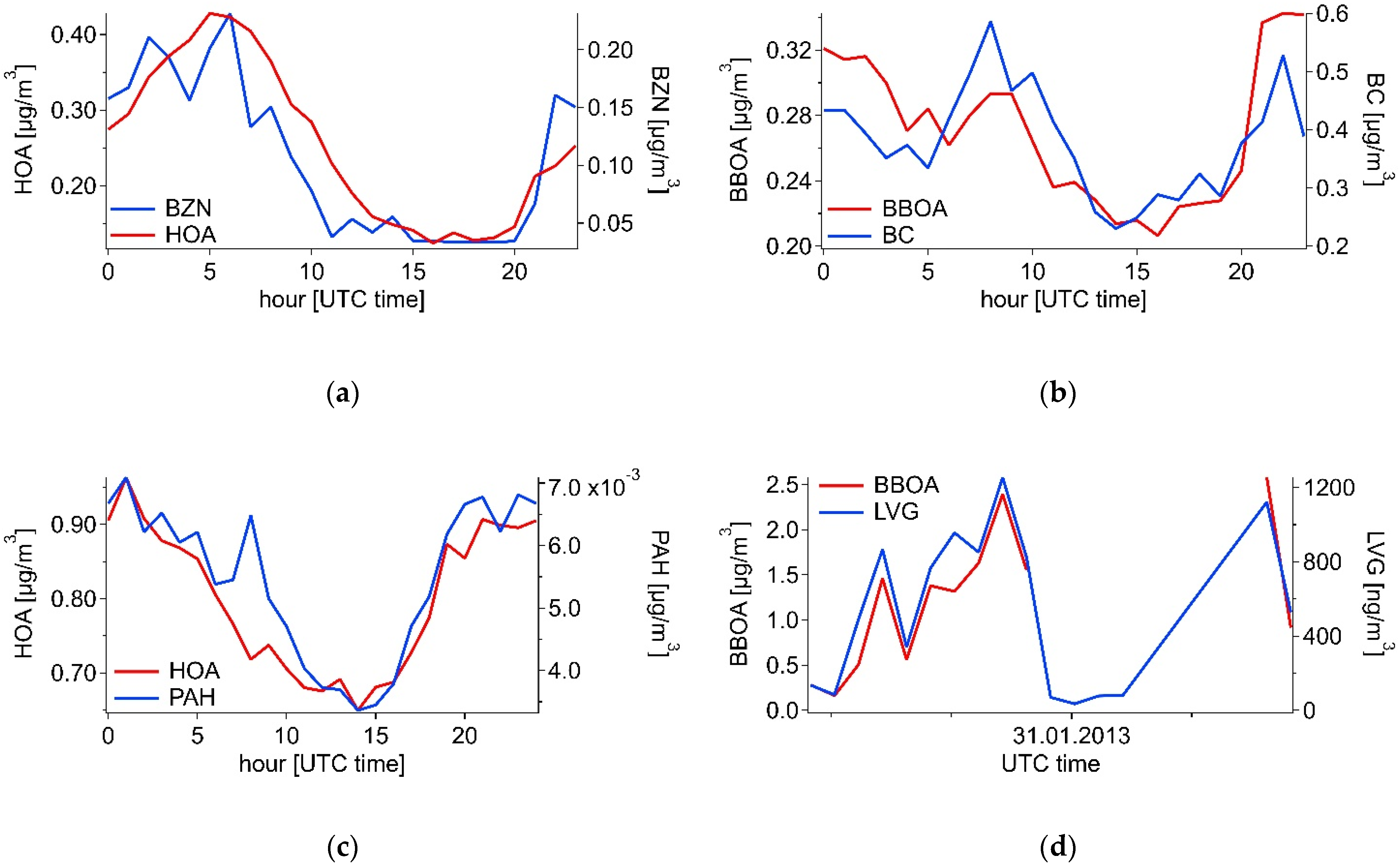
3.2. OA Source Apportionment

3.2.1. Summer

During the summer season, the model identified four factors, which are shown in Figure 2a. An attempt to find a solution with five factors was interpreted as a split of a factor previously identified. At the same time, the five-factor solution practically did not contribute at all to explaining the variance of the data, and the changing of Q / Q e x p value was also negligible. Two factors consisting mainly of fresh aerosol (POA) were identified as hydrocarbon-like organic aerosol (HOA) and biomass-burning organic aerosol (BBOA). The remaining two factors consisting of secondary aerosol were identified as oxygenated organic aerosol 1 (OOA1) and oxygenated organic aerosol 2 (OOA2).
The HOA factor which is associated with fresh traffic emissions is characterised by typical mass to charge ratios of m/z 41, 42, and 43. Furthermore, masses m/z 53, 55, 57, and 71 are present, while m/z 60 and m/z 73, which are typical markers of biomass burning, are absent. The BBOA factor is typically composed of fresh emissions from biomass burning. This factor is characterised by a significant contribution of m/z 60 and m/z 73, which are formed in the presence of anhydrosugars such as levoglucosan [60,61]. Other BBOA factor masses with higher contributions include m/z 41, 44, 55, and 57, which are composed of unoxidised m/z fragments CxHy+. Another POA factor that is frequently found in urban areas is cooking organic aerosol (COA). However, this was not identified in the results based on mass profile and there is also no evidence of COA factor daily pattern in residues [21]. Both OOA factors have quite similar mass profiles with a dominant mass m/z 44, however, the OOA2 factor contains a high proportion of m/z 29, which is mainly composed of partially oxidised CHO+ ion and also has a slightly higher proportion of m/z 55. The average diurnal cycles of the individual factors in both seasons are shown in Figure S2a,b.
Figure 3 confirms the validity of the model results because the time courses of the identified POA factors correspond to the time courses of their tracers. Figure 3a shows the daily pattern of the HOA factor and benzene, which is a good tracer of traffic in the summer season due to higher photo-oxidation and the absence of house heating [62,63]. Figure 3b shows the daily pattern of the BBOA factor and BC as a tracer of combustion processes [64,65].

3.2.2. Winter

During the winter season, four factors were also identified (Figure 2b). The HOA profile differs from the summer profile mainly by the presence of m/z 44 and at lower concentrations also m/z 55 and m/z 57. In the BBOA profile, the m/z 28 and m/z 44 disappeared, compared with the summer, and instead, m/z 43 was strongly present in the factor. As in the summer season, the calculated concentrations of POA factors were validated by comparing the time courses of their concentrations with the tracer concentrations of these factors. Daily patterns of HOA factor and PAHs as a tracer for combustion processes [66] are shown in Figure 3c. Figure 3d shows the daily pattern of the BBOA factor and its tracer levoglucosan [67]. Levoglucosan concentration data were not available during the summer season; thus, the BBOA was compared with the BC course. In all four graphs of Figure 3, we can see that the time courses of the identified factors in both seasons follow the courses of their tracers. The differences in the time courses of the factors and their tracers are due to the fact that although the tracers for each factor are significant, they are not exclusive. This means that these chemical compounds may be formed by different processes.
While the two remaining SOA factors have very similar mass profiles, they can be well distinguished according to the directions from which their air masses come and the prevailing wind speeds. Figure 4a shows that while the factor labelled long-range oxygenated organic aerosol (LROOA) has similar aerosol concentrations from all directions, while the factor labelled local oxygenated organic aerosol (LOOA) (Figure 4b) has the highest contributions from the west, northwest, and north. Furthermore, we can see in Figure 4a that low contributions of the LROOA fraction do not occur at higher wind speeds. Thus, it can be assumed that the LROOA factor represents aerosol from more distant locations, while the LOOA factor has more local character because Figure 4b shows that the LOOA fraction decreases with increasing wind speed. In addition, the residential area adjacent to the measuring station lies in the direction of the highest LOOA concentrations. This inversely proportional relationship between concentration and wind speed was not observed for any SOA factor during the summer season (Figure S3).

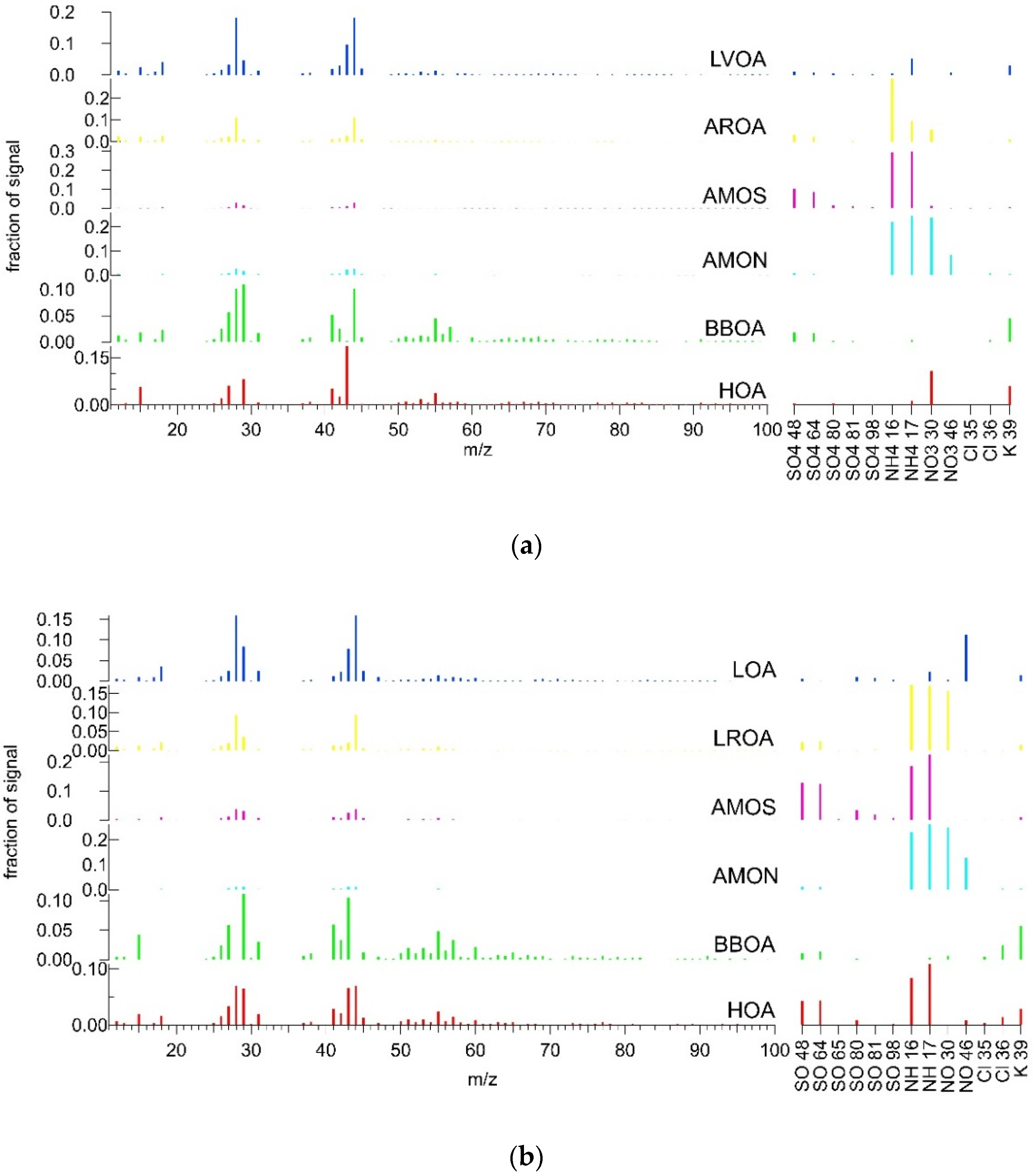
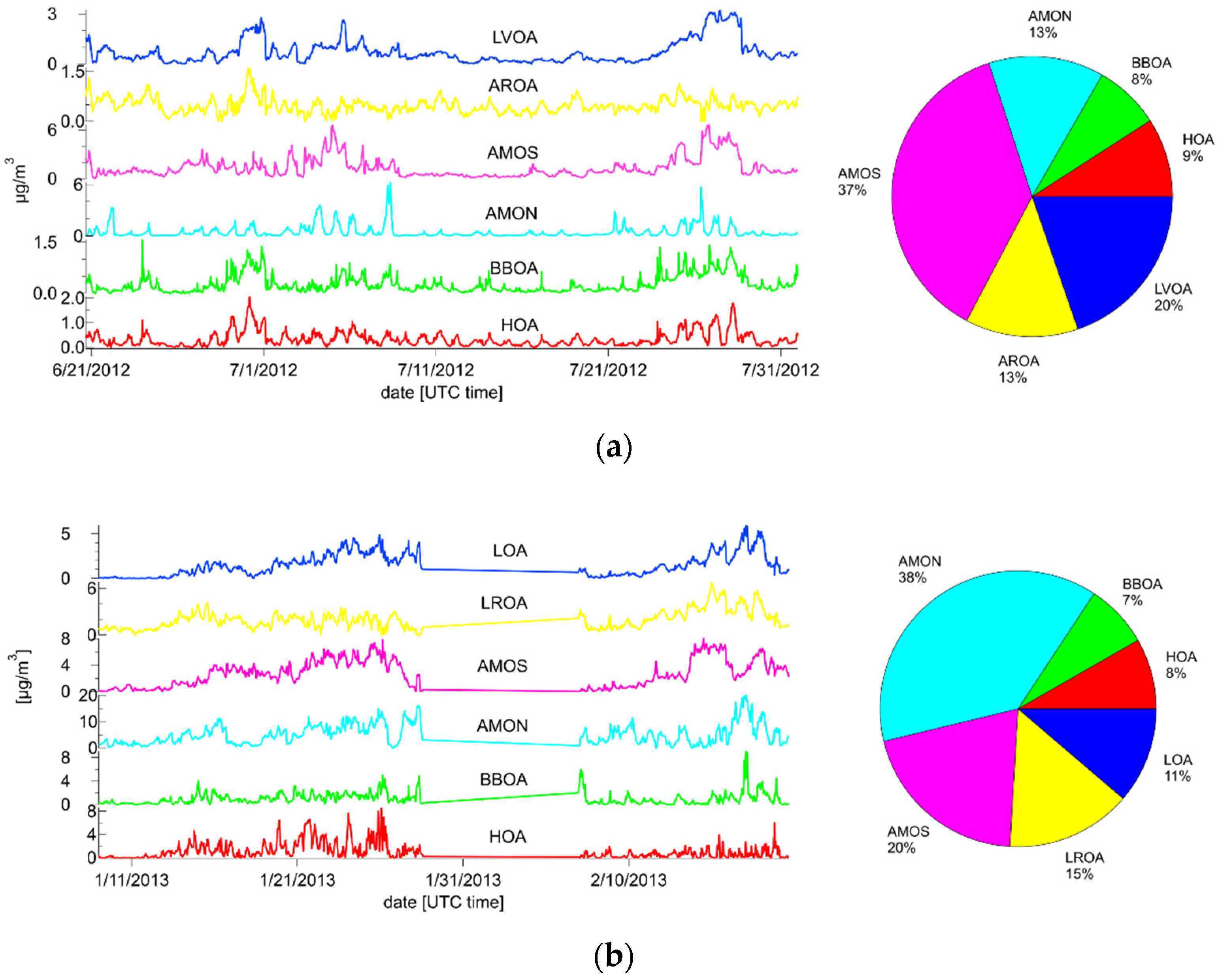
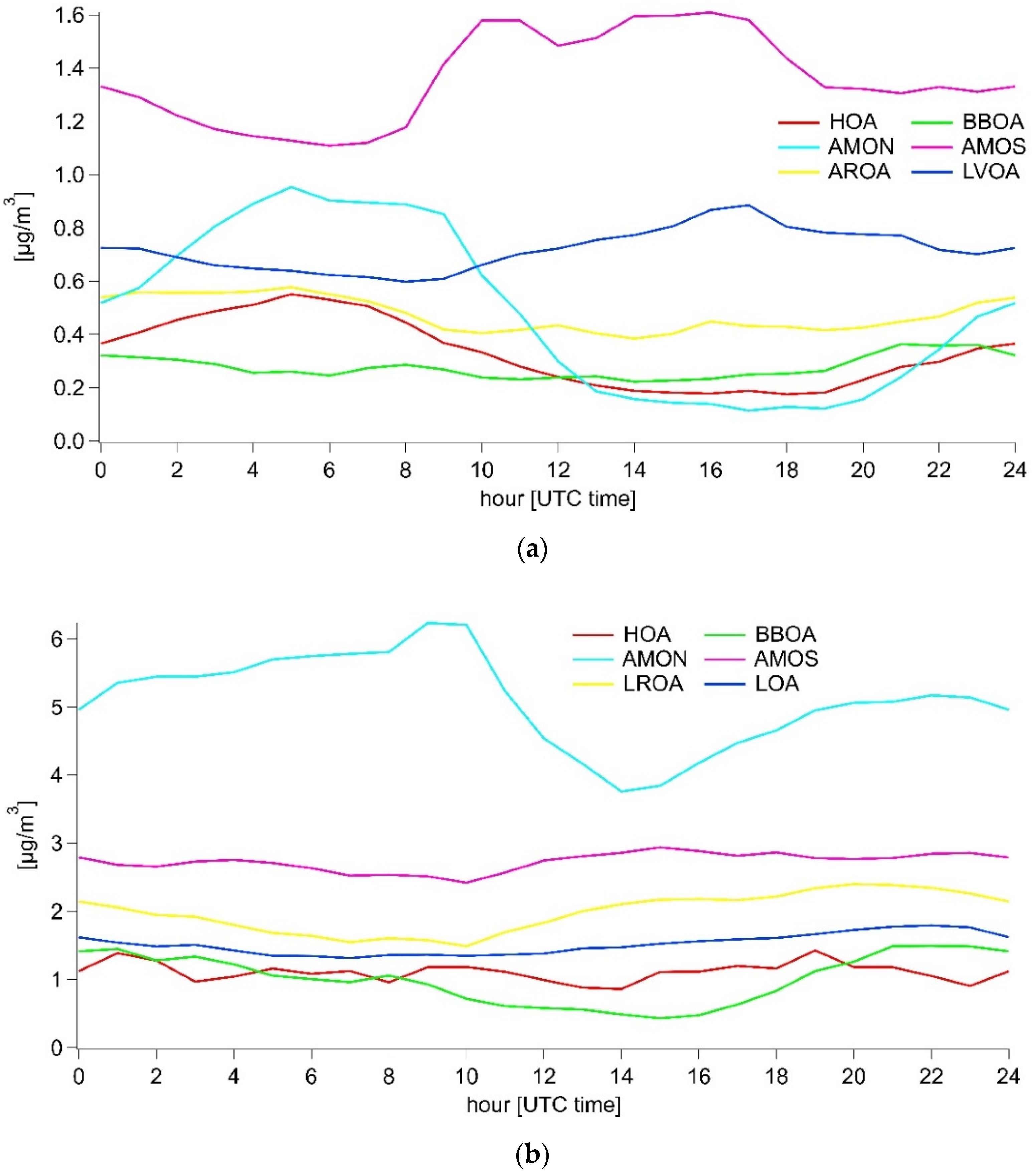
3.3. Combined Spectra Source Apportionment

The HOA and BBOA factors, identified in both seasons during analyses of only the organic parts of the mass spectra, were used as a priori information to determine the factor profiles during the whole mass spectra analysis. These two factors were fixed at a-val = 0.15 for both summer and winter seasons using the a-value method. This value was found to be optimal by analysis of the residuals, which are shown in Figure S4.

3.3.1. Summer

During both seasons, six-factor solutions were identified. This number of factors was selected as the optimum because it showed a better value of Q / Q e x p function and substantial changes in residue structure, compared with the five-factor solution. In contrast, the seven-factor solution had little effect on the model residuals and there was a split in the low-volatile oxygenated aerosol (LVOA) factor that would be difficult to interpret. During both seasons, two factors were consistently identified as dominantly fresh sources, two factors representing more or less aged and oxidised aerosol, and two factors consisting mainly of inorganic aerosol.
Figure 5a, showing the factor loadings during the summer season, displays the HOA factor, which is mainly related to fresh traffic emissions. The organic part of the spectrum is dominated by the typical masses m/z 41, 43, 55. In the inorganic part, the most significant is m/z 30 (NO+), the source of which may be organo-nitrates formed from NOx produced in internal combustion engines [68]. The second important inorganic mass is m/z 39, which for C-ToF AMS is associated only with potassium ion K+. One explanation could be that it is not actually potassium emissions but, for example, the C3H3+ ion, which C-ToF AMS is unable to distinguish and which fits in its nature with the typical fresh hydrocarbon-like profile of CnH2n−1. [69]. However, it can also be potassium, which is used as an additive in gasoline [52,70]. Another identified POA is the BBOA factor, for which the organic part of the spectrum (OS) is typically represented by masses m/z 60 and m/z 73. The inorganic part of the spectrum is dominated by m/z 39, probably composed mainly of K+ ion, which is associated with biomass burning. In addition, sulphate and chloride are present in this part of the spectrum and are also associated with emissions from combustion processes. The other two factors are composed mainly of inorganic ions. The factor named ammonium nitrate (AMON) has the most pronounced peaks at m/z 28 and m/z 44 in the OS. Both NO+ (m/z 30) and NO2+ (m/z 46) nitrate-related masses are strongly represented in the IS, as well as both NH2+ (m/z 16) and NH3+ (m/z 17) ammonium ion-related masses. The ammonium sulphate (AMOS) factor is composed primarily of the sulphate ions SO+ (m/z 48) and SO2+ (m/z 64) and again both ammonium ions. The fifth identified factor was LVOA because the OS profile of the factor with peaks at m/z 28 and m/z 44 agrees with the OOA profiles of the factors published in the literature [37,46,71]. In the IS, the contributions of the individual masses are considerably lower, compared with the OS. The sixth and last factor identified is the ammonia-rich oxygenated aerosol (AROA) factor, which in OS has the highest contributions from oxidised masses m/z 28 and m/z 44 and in IS has the highest contributions in ammonium and nitrate m/z 30. No convincing physical or chemical explanation for this factor has yet been found, and therefore, it can be assumed that this factor is actually just a randomly mixed SOA with part of ammonium nitrate masses, due to the increased difficulty of the calculation by adding the inorganic ions.

3.3.2. Winter

Figure 5b shows the factor profiles during the winter season. When compared with the profiles from the summer season, it can be seen that both winter POA factors have undergone a number of changes. There is a significant addition of mass m/z 44 in the OS of the HOA factor, which, although typical for secondary oxidised aerosol, this mass is also produced during coal combustion as an organic acid fragment, e.g., [72]. An alternative explanation may be that the measuring station is located on the outskirts of the Prague metropolitan area, and therefore, most of the traffic emissions arrive at the station with a delay and are already partially chemically transformed, depending on the current atmospheric conditions such as solar radiation intensity, temperature, and boundary layer height. Furthermore, mass m/z 57 and m/z 60, which also occur in coal combustion, were found at lower concentrations [72]. In addition to potassium, which was also present in the summer season, the chloride ions Cl+ (m/z 35) and HCl+ (m/z 36), the sulphate ions SO+ (m/z 48) and SO2+ (m/z 64), as well as both ammonium ions, and NO2+ instead of NO+ appeared in the IS. These differences in the two parts of the spectra are likely due to the inclusion of fresh emissions from local heating sources in the surrounding residential area, particularly coal-fired boilers, in the HOA factor. These coal emissions could not be identified as a separate source by the model despite considerable effort. For the BBOA factor, the m/z 43 appeared in OS, and m/z 44 disappeared. Then, in IS, the chloride fraction increased significantly, compared with summer. Again, all these changes can be explained by fresh biomass emissions from local heating sources, where many circumstances such as boiler quality, fuel moisture, or air supply to the boiler play a significant role [73], and therefore, emissions from households can vary considerably in time and space. The mass profiles of the two predominantly inorganic factors ammonium nitrate (AMON) and ammonium sulphate (AMOS) hardly differ between seasons. Another factor, which has been named long-range oxygenated aerosol (LROA), does not differ much from summer factor AROA in OS, whereas the contribution of NH+ and NO+ increases in IS, compared with summer. The reasons for naming the factor will be explained below. For the last factor named local oxygenated aerosol (LOA), the main change from the summer LVOA factor is the presence of more oxidised nitrate ion NO2+.
Next, the total aerosol concentrations and timelines of each factor were analysed (Figure 6a). In the summer season, the sum of the primary factors was 17% of the total mass. Of this, HOA accounted for 8% and BBOA for 9%. AROA and LVOA accounted for 13% and 17%, respectively, which together account for almost one-third of the total mass. The remaining half of the mass was accounted for by the factors AMON (13%) and AMOS (37%). The proportion of POA did not change much in the winter season (Figure 6b). The concentrations of HOA and BBOA decreased by one percent, to 7% and 8%, respectively. A relatively low share of primary factors might be surprising in winter, although it must be understood that this share is related to relatively fresh sources, while older oxidised originally primary aerosol is continuously transformed into oxidised aerosol factors. The fraction of LROA increased slightly to 15%, and LOA decreased to 11%. Due to the cold temperatures in winter, volatile ammonium nitrate evaporated less during the day (Figure 7b), and therefore, the proportion of AMON increased to 38%. In contrast, the proportion of AMOS decreased to 20% because SO2 oxidation is slower due to lower photochemical activity in winter.
When investigating the differences in the diurnal cycles of the individual factors between seasons (Figure 7a,b), we can see that the typical morning and evening peaks are not present in the HOA diurnal cycle in the summer season. The likely reasons are changes in the thickness of the atmospheric boundary layer. At night, when the strength of the boundary layer is typically lower, less air volume remains to dilute emissions, and HOA concentrations increase despite weaker traffic. During the winter season, this effect is not so apparent because the difference in boundary layer thickness is not as large [74]. This effect is also observed at a lower scale in summer for the BBOA factor. The shape of the BBOA diurnal cycle curve in the winter season seems to be mainly due to biomass burning in residential boilers.
This assumption is also supported by Figure S5a for HOA and Figure S5b for BBOA. Both graphs show a similar situation, that is, high concentrations of particulate matter at low wind speeds are coming from local residential areas. AROA concentrations in the summer season reach a maximum at around 4 a.m. and a minimum around 2 p.m. (Figure 7a). The shape of the curve is likely to be influenced by the vertical motions of the atmospheric boundary layer. The presence of nitrate and ammonium ions, which can form volatile ammonium nitrate, may also have some influence. LVOA then has its highest concentrations in the afternoon during rush hours. Looking at the rose plot of the LVOA factor (Figure S6a), it can be seen that the highest concentrations come from the SE, E, and NE directions, that is, from the more densely populated directions from which the aerosol arrives at the measuring station already oxidised. Figure S5c shows that particles from the LROA factor were advected from all directions at similar concentrations, but only at higher wind speeds were higher particle concentrations measured. Thus, it can be assumed that the LROA factor in winter represents regional or long-range transport of pollution [31]. This also explains why the LROA curve in Figure 7b does not follow a similar pattern as in the summer season. As mentioned above, the diurnal pattern of the AMON and AMOS factors is opposite due to the volatility of ammonium nitrate and at the same time photochemical formation of sulphate ions or due to vertical mixing of sulphate from the upper boundary layer and the subsequent reaction of ammonia with them. During the winter campaign, the trend is similar, only not as pronounced due to lower air temperatures.
The results of the analysis of the organic parts of the spectra are now compared with the results for the whole spectra within the individual measurement campaigns. Table 1 shows the coefficients of determination (R2) and slopes of a linear fit for pairs of related factors in both seasons.
Regarding the method of fixing the HOA and BBOA factors in the analysis of the combined spectra, high R2 values are expected at least for these factors. However, the remaining unfixed factors of the combined spectrum analysis also achieve R2 > 95% during both seasons. The slope of a linear fit of the HOA/HOA and LROA/LROOA factors during the winter campaign shows that the factor loadings of the organic part of the combined profiles of HOA and LROA, respectively, are approximately half those of the same factors of the organic spectra. For the BBOA/BBOA and LOA/LOOA factors, this reduction is only around 15% and 5%, respectively. In the results from the summer campaign, this trend is also evident to a lesser extent. This phenomenon is probably because the results of the analysis of the combined spectra contain two additional factors AMOS and AMON. Although their profiles are predominantly inorganic, the AMOS factor, in particular, contains a significant amount of organic matter that may be associated with coal combustion [75,76], consistent with the decline in the HOA factor during the winter season.
If we compare the diurnal cycles of the results of the organic spectra analyses with the combined spectra in the summer season (Table 2) (Figure S7), we see that the R2 ranges from 0.73 for the AROA/OOA1 factors to 0.98 for the HOA/HOA factors, indicating a high agreement between the results of the two analyses. The situation changes in the winter season (Figure S7). While the BBOA and LROA/LROOA factors show a high agreement of daily trends (BBOA/BBOA: R2 = 0.98, LROA/LROOA: R2 = 0.71), for the daily patterns of the HOA factors the R2 = 0.16 and for LOA/LOOA the R2 = 0.1. The variation in the diurnal cycles of the HOA factor in Figure S7 shows how the addition of the inorganic part of the spectrum can cause failure in the identification of factors. The top right graph of Figure S7 shows the daily trend of HOA_all, which is very noisy. Considering Table 1, it can be assumed that these different behaviours are mainly due to inorganic ions. Aerosol particles in the atmosphere are constantly undergoing various chemical reactions, and it may, therefore, be difficult for the model to accurately assign the reacted ions to the original aerosol source. Moreover, the situation in winter is complicated by the combustion of different types of solid fuels under different combustion conditions.
Since 2012, when the first part of the measurement campaign began, the vehicle fleet has been gradually renewed. In addition, in 2015, a state programme of financial support for the replacement of old domestic solid fuel boilers was started, but it was primarily targeted at other regions than the capital city of Prague. Nevertheless, CHMI annual reports show that air quality is improving only very slightly between 2011 and 2021, and the impact of the trends described above on air quality is lost in the climatic specifics of individual years, which affect, for example, the length of the heating season. It can, therefore, be assumed that the results of this measurement campaign will be still valid in 2021.
Finally, the methodology used in this study, which is described in Section 2.3, is compared with the approaches used in the papers by Sun [77] and Äijälä [78]. Sun, unlike our approach, does not utilise a mass profile fixing method to optimise the solution but uses a method called FPEAK to control the rotational ambiguity of the resulting factors. This approach may be appropriate when the data have low noise, and there are no problems with the convergence of the solutions. The approach of Äijälä is more similar to ours, but it includes one extra step. In the first and second steps, consistent with our model, he identifies potential solutions using PMF, which is then refined using the ME-2 algorithm. In the third step, a CMB approach is used in which all the found mass profiles are fixed, and their time series are calculated. The reason for using this more complex model is that Äijälä analyses a long time series involving data over four years. This model better reflects the seasonality of some sources.

4. Summary and Conclusions

This paper analysed data measured by C-ToF AMS during the summer and winter six-week campaigns in the suburbs of Prague. At first, only the organic parts of the mass spectra were analysed using the PMF method. In the next step, these results were used as additional inputs to refine the ME-2 analysis of the whole mass spectra including inorganic ions. The results were then discussed in terms of the differences between seasons as well as through the differences between the analyses of the organic and combined spectra within the same season.
When analysing the mass spectra of organic ions only, four factors were identified in both seasons, two of which were primary, and two were secondary. In the summer season, these were the HOA factor (15.1%) originating mainly from traffic, the BBOA factor (15.9%), and two factors representing oxidised organic aerosols OOA1 (31.3%) and OOA2 (37.7%). Fresh HOA and BBOA factors were also identified in winter. The difference, however, is that in winter, coal combustion contributes to the HOA factor (16.3%), in addition to transport, and wood combustion in residential boilers contributes to the BBOA factor (21%). Furthermore, the LROOA factor (40.4%) was identified in winter, which represents the long-range and regional transport of oxidised aerosol. The last winter factor representing oxidised aerosol generated in the vicinity of the measuring station is LOOA (22.4%). These two factors were distinguished based on their dependence on wind speed.
Analyses of whole mass spectra combining organic and inorganic ions resulted in six-factor solutions in both seasons. In addition to the four factors whose organic parts of the profiles closely match the results of the organic spectra analysis, two factors involving mainly inorganic ions were added in both summer and winter. One is the AMON factor representing nitrate and ammonium ions, and the other is the AMOS factor containing sulphate and ammonium ions. These two inorganic factors varied only slightly between seasons. The HOA and BBOA factors, again identified in both seasons, showed some differences between seasons due to the combustion of solid fuels during the winter season. The other two factors in summer are AROA and LVOA, which are ammonium ion enriched oxidised aerosol and low volatile oxidised aerosol, respectively. In winter, the LROA factor, representing regional and long-range transport, and the LOA factor including oxidised aerosol from local sources complete the six factors. Although the organic spectrum factors have very similar profiles to the combined spectrum factors, their diurnal cycles differ considerably in some cases, especially in the winter season. Specifically, the daily runs of the HOA factors and the local oxidised aerosol factors show very low agreement, probably due to higher noise caused by inorganic ions that affect the complexity of the calculation.
The aim of the study was to extend the description of aerosol sources to include an inorganic part in order to obtain more comprehensive information on the size and chemical composition of AA sources. However, when comparing organic and combined analyses, the combined approach provided similar results, without adding any substantial improvement to the solution in the organic part and, on the other hand, resulting in a worse identification of HOA in winter and AROA in summer, which is not fully explainable. To conclude, the knowledge of the source contribution in the inorganic part of the spectrum is compensated by a worse identification of the organic part of the spectrum. Further research is needed to develop a reliable and robust methodology for source apportionment of both the organic and inorganic parts of the AMS mass spectra.

Supplementary Materials

The following are available online at https://www.mdpi.com/article/10.3390/atmos13010020/s1, Figure S1: Wind roses: (a) wind velocity (top left) and (b) directionality of PM1 aerosol (top right) in summer season; (c) wind velocity (bottom left) and (d) directionality of PM1 aerosol (bottom right) in winter season, Figure S2. (a,b) Averaged daily cycles of individual factors in summer (top) and winter (bottom) obtained from the analysis of organic spectra, Figure S3. Dependence of the proportion of (a) OOA1 fraction and (b) OOA2 fractions on wind speed. Fractions are obtained as a proportion of a factor to the total mass of all factors, Figure S4. (a,b) Time series (top) and diurnal cycles (bottom) of residues obtained from analysis of combined mass spectra during the summer season. (c,d) Time series (top) and diurnal cycles (bottom) of residues obtained from analysis of combined mass spectra during the winter season, Figure S5. (a,b) Dependence of proportion of HOA (top) and BBOA (bottom) fractions on wind speed. Fractions are obtained as a proportion of a factor to the total mass of all factors. The graphs also contain wind roses showing the directionality of the factors. (c) Dependence of proportion of LROA fraction on wind speed. Fraction is obtained as the proportion of a factor LROA to the total mass of all factors. The graph also contains wind rose showing the directionality of the factor LROA, Figure S6. (a) Directionality of all factors obtained from combined mass spectra analysis for summer season. (b) Directionality of all factors obtained from combined mass spectra analysis for winter season, Figure S7. Comparison of the average diurnal cycles of the factors obtained by analysing the organic part of the spectra and the combined spectra. The blue colour indicates the results for the combined spectra, and the red colour indicates the organic spectra. The r2 value indicates the linear fit expressed by the coefficient of determination.

Author Contributions

Conceptualisation, J.S. and V.Ž.; methodology, J.S. and V.Ž.; analysis, O.M., P.V. and G.E.; writing, O.M.; supervision, J.S. All authors have read and agreed to the published version of the manuscript.

Funding

This research was funded by Czech Science Foundation, Grant Number CSF P209/11/1342, and Meys’s Inter-Excellence Intercost programme, under Grant No. LTC18068; the APC was funded by Actris CZ LM2018122.

Institutional Review Board Statement

Not applicable.

Informed Consent Statement

Not applicable.

Acknowledgments

The meteorological data provided by Czech Hydrometeorological Institute is gratefully appreciated.

Conflicts of Interest

The authors declare no conflict of interest.

Abbreviations

AAAtmospheric Aerosol
AIMAutomated Immission Monitoring
AMONAmmonium Nitrate
AMOSAmmonium Sulphate
AMSAerosol Mass Spectrometer
AROAAmmonia Rich Oxygenated Aerosol
ASLAbove Sea Level
BBOABiomass Burning Organic Aerosol
BCBlack Carbon
CECollection Efficiency
CHMICzech Hydrometeorological Institute
CMBChemical Mass Balance
COACooking Organic Aerosol
HOAHydrocarbon-like Organic Aerosol
IAInorganic Aerosol
LOALocal Oxygenated Aerosol
LOOALocal Oxygenated Organic Aerosol
LROALong Range Oxygenated Aerosol
LROOALong Range Oxygenated Organic Aerosol
LVOALow Volatile Oxygenated Aerosol
ME-2Multilinear Engine
NRNon-refractory
OAOrganic Aerosol
OOA1Oxygenated Organic Aerosol 1
OOA2Oxygenated Organic Aerosol 2
PAHsPolycyclic Aromatic Hydrocarbons
PCAPrincipal Component Analysis
PMFPositive Matrix Factorization
PMXParticulate Matter with diameter smaller than X
POAPrimary Organic Aerosol
R2Coefficient of determination
SOASecondary Organic Aerosol
UMRUnit Mass Resolution

References

  1. Engling, G.; Gelencsér, A. Atmospheric Brown Clouds: From Local Air Pollution to Climate Change. Elements 2010, 6, 223–228. [Google Scholar] [CrossRef]
  2. IPCC. Climate Change 2014: Mitigation of Climate Change; IPCC: Geneva, Switzerland, 2014. [Google Scholar]
  3. Singh, A.; Dey, S. Influence of aerosol composition on visibility in megacity Delhi. Atmos. Environ. 2012, 62, 367–373. [Google Scholar] [CrossRef]
  4. Tuckermann, R.; Cammenga, H.K. The surface tension of aqueous solutions of some atmospheric water-soluble organic compounds. Atmos. Environ. 2004, 38, 6135–6138. [Google Scholar] [CrossRef]
  5. Pan, C.; Zhu, B.; Fang, C.; Kang, H.; Kang, Z.; Chen, H.; Liu, D.; Hou, X. The Fast Response of the Atmospheric Water Cycle to Anthropogenic Black Carbon Aerosols during Summer in East Asia. J. Clim. 2021, 34, 3049–3065. [Google Scholar] [CrossRef]
  6. Pope, C.A., 3rd; Dockery, D.W. Health Effects of Fine Particulate Air Pollution: Lines that Connect. J. Air Waste Manag. Assoc. 2006, 56, 709–742. [Google Scholar] [CrossRef] [PubMed]
  7. Butt, E.W.; Rap, A.; Schmidt, A.; Scott, C.E.; Pringle, K.J.; Reddington, C.L.; Richards, N.A.D.; Woodhouse, M.T.; Ramirez-Villegas, J.; Yang, H.; et al. The impact of residential combustion emissions on atmospheric aerosol, human health, and climate. Atmos. Chem. Phys. Discuss. 2016, 16, 873–905. [Google Scholar] [CrossRef] [Green Version]
  8. Seinfeld, J.H.; Pandis, S.N. Atmospheric Chemistry and Physics: From Air Pollution to Climate Change, 3rd ed.; John Wiley & Sons: New York, NY, USA, 2016. [Google Scholar]
  9. Jimenez, J.L.; Canagaratna, M.R.; Donahue, N.M.; Prevot, A.S.H.; Zhang, Q.; Kroll, J.H.; Decarlo, P.F.; Allan, J.D.; Coe, H.; Ng, N.L.; et al. Evolution of Organic Aerosols in the Atmosphere. Science 2009, 326, 1525–1529. [Google Scholar] [CrossRef] [PubMed]
  10. Jayne, J.T.; Leard, D.C.; Zhang, X.; Davidovits, P.; Smith, K.A.; Kolb, C.E.; Worsnop, D.R. Development of an Aerosol Mass Spectrometer for Size and Composition Analysis of Submicron Particles. Aerosol Sci. Technol. 2000, 33, 49–70. [Google Scholar] [CrossRef] [Green Version]
  11. Jimenez, J.L.; Jayne, J.T.; Shi, Q.; Kolb, C.E.; Worsnop, D.R.; Yourshaw, I.; Seinfeld, J.H.; Flagan, R.C.; Zhang, X.; Smith, K.A.; et al. Ambient aerosol sampling using the Aerodyne Aerosol Mass Spectrometer. J. Geophys. Res. Space Phys. 2003, 108. [Google Scholar] [CrossRef] [Green Version]
  12. Allan, J.D.; Delia, A.E.; Coe, H.; Bower, K.; Alfarra, R.; Jimenez, J.L.; Middlebrook, A.; Drewnick, F.; Onasch, T.B.; Canagaratna, M.R.; et al. A generalised method for the extraction of chemically resolved mass spectra from Aerodyne aerosol mass spectrometer data. J. Aerosol Sci. 2004, 35, 909–922. [Google Scholar] [CrossRef]
  13. Watson, J.G.; Zhu, T.; Chow, J.C.; Engelbrecht, J.; Fujita, E.M.; E Wilson, W. Receptor modeling application framework for particle source apportionment. Chemosphere 2002, 49, 1093–1136. [Google Scholar] [CrossRef] [Green Version]
  14. Roweis, S.T.; Saul, L.K.; Roweis, S.T.; Saul, L.K. Linked references are available on JSTOR for this article: Nonlinear Nonlinear Dimensionality Dimensionality Reduction by Locally Linear Embedding. Science 2000, 290, 2323–2326. [Google Scholar] [CrossRef] [PubMed] [Green Version]
  15. Paatero, P.; Tapper, U. Positive matrix factorization: A non-negative factor model with optimal utilization of error estimates of data values. Environmetrics 1994, 5, 111–126. [Google Scholar] [CrossRef]
  16. Paatero, P. Least squares formulation of robust non-negative factor analysis. Chemom. Intell. Lab. Syst. 1997, 37, 23–35. [Google Scholar] [CrossRef]
  17. Zhang, Q.; Jimenez, J.L.; Canagaratna, M.R.; Ulbrich, I.M.; Ng, N.L.; Worsnop, D.R.; Sun, Y. Understanding atmospheric organic aerosols via factor analysis of aerosol mass spectrometry: A review. Anal. Bioanal. Chem. 2011, 401, 3045–3067. [Google Scholar] [CrossRef] [Green Version]
  18. Canonaco, F.; Crippa, M.; Slowik, J.G.; Baltensperger, U.; Prévôt, A.S.H. SoFi, an IGOR-based interface for the efficient use of the generalized multilinear engine (ME-2) for the source apportionment: ME-2 application to aerosol mass spectrometer data. Atmos. Meas. Tech. 2013, 6, 3649–3661. [Google Scholar] [CrossRef] [Green Version]
  19. Srivastava, D.; Daellenbach, K.; Zhang, Y.; Bonnaire, N.; Chazeau, B.; Perraudin, E.; Gros, V.; Lucarelli, F.; Villenave, E.; Prévôt, A.; et al. Comparison of five methodologies to apportion organic aerosol sources during a PM pollution event. Sci. Total Environ. 2020, 757, 143168. [Google Scholar] [CrossRef]
  20. Lanz, V.A.; Prévôt, A.S.H.; Alfarra, M.R.; Weimer, S.; Mohr, C.; DeCarlo, P.F.; Gianini, M.F.D.; Hueglin, C.; Schneider, J.; Favez, O.; et al. Characterization of aerosol chemical composition with aerosol mass spectrometry in Central Europe: An overview. Atmos. Chem. Phys. Discuss. 2010, 10, 10453–10471. [Google Scholar] [CrossRef] [Green Version]
  21. Mohr, C.; DeCarlo, P.F.; Heringa, M.F.; Chirico, R.; Slowik, J.G.; Richter, R.; Reche, C.; Alastuey, A.; Querol, X.; Seco, R.; et al. Identification and quantification of organic aerosol from cooking and other sources in Barcelona using aerosol mass spectrometer data. Atmos. Chem. Phys. Discuss. 2012, 12, 1649–1665. [Google Scholar] [CrossRef] [Green Version]
  22. Crippa, M.; Canonaco, F.; Lanz, V.A.; Äijälä, M.; Allan, J.D.; Carbone, S.; Capes, G.; Ceburnis, D.; Dall’Osto, M.; Day, D.A.; et al. Organic aerosol components derived from 25 AMS data sets across Europe using a consistent ME-2 based source apportionment approach. Atmos. Chem. Phys. Discuss. 2014, 14, 6159–6176. [Google Scholar] [CrossRef] [Green Version]
  23. Ots, R.; Vieno, M.; Allan, J.D.; Reis, S.; Nemitz, E.; Young, D.E.; Coe, H.; Di Marco, C.; Detournay, A.; Mackenzie, I.A.; et al. Model simulations of cooking organic aerosol (COA) over the UK using estimates of emissions based on measurements at two sites in London. Atmos. Chem. Phys. Discuss. 2016, 16, 13773–13789. [Google Scholar] [CrossRef] [Green Version]
  24. Tobler, A.K.; Canonaco, F.; Skiba, A.; Močnik, G.; Pragati, R.; Styszko, K.; Nęcki, J.; Slowik, J.G.; Baltensperger, U.; Prevot, A.S.H.; et al. Characterization of non-refractory (NR) PM1 and source apportionment of organic aerosol in Kraków, Poland. Atmos. Chem. Phys. 2021, 21, 14893–14906. [Google Scholar] [CrossRef]
  25. Poulain, L.; Fahlbusch, B.; Spindler, G.; Müller, K.; van Pinxteren, D.; Wu, Z.; Iinuma, Y.; Birmili, W.; Wiedensohler, A.; Herrmann, H. Source apportionment and impact of long-range transport on carbonaceous aerosol particles in central Germany during HCCT-2010. Atmos. Chem. Phys. Discuss. 2021, 21, 3667–3684. [Google Scholar] [CrossRef]
  26. Schwarz, J.; Pokorná, P.; Rychlík, Š.; Škáchová, H.; Vlček, O.; Smolík, J.; Ždímal, V.; Hůnová, I. Assessment of air pollution origin based on year-long parallel measurement of PM2.5 and PM10 at two suburban sites in Prague, Czech Republic. Sci. Total Environ. 2019, 664, 1107–1116. [Google Scholar] [CrossRef] [PubMed]
  27. Pokorná, P.; Hovorka, J.; Hopke, P.K. Elemental composition and source identification of very fine aerosol particles in a European air pollution hot-spot. Atmos. Pollut. Res. 2016, 7, 671–679. [Google Scholar] [CrossRef]
  28. Leoni, C.; Pokorná, P.; Hovorka, J.; Masiol, M.; Topinka, J.; Zhao, Y.; Krumal, K.; Cliff, S.; Mikuška, P.; Hopke, P.K. Source apportionment of aerosol particles at a European air pollution hot spot using particle number size distributions and chemical composition. Environ. Pollut. 2018, 234, 145–154. [Google Scholar] [CrossRef] [PubMed]
  29. Vodička, P.; Schwarz, J.; Ždímal, V. Analysis of one year’s OC/EC data at a Prague suburban site with 2-h time resolution. Atmos. Environ. 2013, 77, 865–872. [Google Scholar] [CrossRef]
  30. Vodička, P.; Kawamura, K.; Schwarz, J.; Ždímal, V. Seasonal changes in stable carbon isotopic composition in the bulk aerosol and gas phases at a suburban site in Prague. Sci. Total Environ. 2021, 803, 149767. [Google Scholar] [CrossRef] [PubMed]
  31. Kubelová, L.; Vodička, P.; Schwarz, J.; Cusack, M.; Makeš, O.; Ondráček, J.; Ždímal, V. A study of summer and winter highly time-resolved submicron aerosol composition measured at a suburban site in Prague. Atmos. Environ. 2015, 118, 45–57. [Google Scholar] [CrossRef]
  32. Horník, Š.; Sýkora, J.; Pokorná, P.; Vodička, P.; Schwarz, J.; Ždímal, V. Detailed NMR analysis of water-soluble organic compounds in size-resolved particulate matter seasonally collected at a suburban site in Prague. Atmos. Environ. 2021, 267, 118757. [Google Scholar] [CrossRef]
  33. Drewnick, F.; Hings, S.S.; Decarlo, P.; Jayne, J.T.; Gonin, M.; Fuhrer, K.; Weimer, S.; Jimenez, J.L.; Demerjian, K.L.; Borrmann, S.; et al. A New Time-of-Flight Aerosol Mass Spectrometer (TOF-AMS)—Instrument Description and First Field Deployment. Aerosol Sci. Technol. 2005, 39, 637–658. [Google Scholar] [CrossRef]
  34. Zíková, N.; Vodička, P.; Ludwig, W.; Hitzenberger, R.; Schwarz, J. On the use of the field Sunset semi-continuous analyzer to measure equivalent black carbon concentrations. Aerosol Sci. Technol. 2016, 50, 284–296. [Google Scholar] [CrossRef] [Green Version]
  35. Zhang, Z.-S.; Engling, G.; Chan, C.-Y.; Yang, Y.-H.; Lin, M.; Shi, S.; He, J.; Li, Y.-D.; Wang, X.-M. Determination of isoprene-derived secondary organic aerosol tracers (2-methyltetrols) by HPAEC-PAD: Results from size-resolved aerosols in a tropical rainforest. Atmos. Environ. 2013, 70, 468–476. [Google Scholar] [CrossRef]
  36. Dzepina, K.; Arey, J.; Marr, L.C.; Worsnop, D.R.; Salcedo, D.; Zhang, Q.; Onasch, T.B.; Molina, L.T.; Molina, M.J.; Jimenez, J.L. Detection of particle-phase polycyclic aromatic hydrocarbons in Mexico City using an aerosol mass spectrometer. Int. J. Mass Spectrom. 2007, 263, 152–170. [Google Scholar] [CrossRef]
  37. Lanz, V.A.; Alfarra, M.R.; Baltensperger, U.; Buchmann, B.; Hueglin, C.; Prévôt, A.S.H. Source apportionment of submicron organic aerosols at an urban site by factor analytical modelling of aerosol mass spectra. Atmos. Chem. Phys. Discuss. 2007, 7, 1503–1522. [Google Scholar] [CrossRef] [Green Version]
  38. Fröhlich, R.; Cubison, M.J.; Slowik, J.G.; Bukowiecki, N.; Canonaco, F.; Croteau, P.L.; Gysel, M.; Henne, S.; Herrmann, E.; Jayne, J.T.; et al. Fourteen months of on-line measurements of the non-refractory submicron aerosol at the Jungfraujoch (3580 m a.s.l.)—Chemical composition, origins and organic aerosol sources. Atmos. Chem. Phys. Discuss. 2015, 15, 18225–18284. [Google Scholar] [CrossRef] [Green Version]
  39. Bressi, M.; Cavalli, F.; Putaud, J.; Fröhlich, R.; Petit, J.-E.; Aas, W.; Äijälä, M.; Alastuey, A.; Allan, J.; Aurela, M.; et al. A European aerosol phenomenology—7: High-time resolution chemical characteristics of submicron particulate matter across Europe. Atmos. Environ. X 2021, 10, 100108. [Google Scholar] [CrossRef]
  40. Canonaco, F.; Tobler, A.; Chen, G.; Sosedova, Y.; Slowik, J.G.; Bozzetti, C.; Daellenbach, K.R.; El Haddad, I.; Crippa, M.; Huang, R.-J.; et al. A new method for long-term source apportionment with time-dependent factor profiles and uncertainty assessment using SoFi Pro: Application to 1 year of organic aerosol data. Atmos. Meas. Tech. 2021, 14, 923–943. [Google Scholar] [CrossRef]
  41. Paatero, P. The Multilinear Engine—A Table-Driven, Least Squares Program for Solving Multilinear Problems, Including then-Way Parallel Factor Analysis Model. J. Comput. Graph. Stat. 1999, 8, 854–888. [Google Scholar] [CrossRef]
  42. Allan, J.; Jimenez, J.L.; Williams, P.; Alfarra, M.R.; Bower, K.; Jayne, J.T.; Coe, H.; Worsnop, D.R. Quantitative sampling using an Aerodyne aerosol mass spectrometer 1. Techniques of data interpretation and error analysis. J. Geophys. Res. Space Phys. 2003, 108, 4090. [Google Scholar] [CrossRef]
  43. Paatero, P.; Hopke, P.; Song, X.-H.; Ramadan, Z. Understanding and controlling rotations in factor analytic models. Chemom. Intell. Lab. Syst. 2002, 60, 253–264. [Google Scholar] [CrossRef]
  44. Ulbrich, I.M.; Canagaratna, M.R.; Zhang, Q.; Worsnop, D.R.; Jimenez, J.L. Interpretation of organic components from Positive Matrix Factorization of aerosol mass spectrometric data. Atmos. Chem. Phys. Discuss. 2009, 9, 2891–2918. [Google Scholar] [CrossRef] [Green Version]
  45. Paatero, P.; Hopke, P.K. Discarding or downweighting high-noise variables in factor analytic models. Anal. Chim. Acta 2003, 490, 277–289. [Google Scholar] [CrossRef]
  46. Crippa, M.; DeCarlo, P.F.; Slowik, J.G.; Mohr, C.; Heringa, M.F.; Chirico, R.; Poulain, L.; Freutel, F.; Sciare, J.; Cozic, J.; et al. Wintertime aerosol chemical composition and source apportionment of the organic fraction in the metropolitan area of Paris. Atmos. Chem. Phys. Discuss. 2013, 13, 961–981. [Google Scholar] [CrossRef] [Green Version]
  47. Canagaratna, M.R.; Jayne, J.T.; Ghertner, D.A.; Herndon, S.; Shi, Q.; Jimenez, J.L.; Silva, P.; Williams, P.; Lanni, T.; Drewnick, F.; et al. Chase Studies of Particulate Emissions from in-use New York City Vehicles. Aerosol Sci. Technol. 2004, 38, 555–573. [Google Scholar] [CrossRef]
  48. Aiken, A.C.; DeCarlo, P.F.; Jimenez, J.L. Elemental Analysis of Organic Species with Electron Ionization High-Resolution Mass Spectrometry. Anal. Chem. 2007, 79, 8350–8358. [Google Scholar] [CrossRef] [PubMed]
  49. Alfarra, M.R.; Prevot, A.S.H.; Szidat, S.; Sandradewi, J.; Weimer, S.; Lanz, V.A.; Schreiber, D.; Mohr, M.; Baltensperger, U. Identification of the Mass Spectral Signature of Organic Aerosols from Wood Burning Emissions. Environ. Sci. Technol. 2007, 41, 5770–5777. [Google Scholar] [CrossRef]
  50. Ng, N.L.; Canagaratna, M.R.; Zhang, Q.; Jimenez, J.L.; Tian, J.; Ulbrich, I.M.; Kroll, J.H.; Docherty, K.S.; Chhabra, P.S.; Bahreini, R.; et al. Organic aerosol components observed in Northern Hemispheric datasets from Aerosol Mass Spectrometry. Atmos. Chem. Phys. 2010, 10, 4625–4641. [Google Scholar] [CrossRef] [Green Version]
  51. Crippa, M.; Canonaco, F.; Slowik, J.G.; El Haddad, I.; DeCarlo, P.F.; Mohr, C.; Heringa, M.F.; Chirico, R.; Marchand, N.; Temime-Roussel, B.; et al. Primary and secondary organic aerosol origin by combined gas-particle phase source apportionment. Atmos. Chem. Phys. Discuss. 2013, 13, 8411–8426. [Google Scholar] [CrossRef] [Green Version]
  52. Schwarz, J.; Cusack, M.; Karban, J.; Chalupníčková, E.; Havránek, V.; Smolík, J.; Ždímal, V. PM2.5 chemical composition at a rural background site in Central Europe, including correlation and air mass back trajectory analysis. Atmos. Res. 2016, 176–177, 108–120. [Google Scholar] [CrossRef]
  53. Štefancová, L.; Schwarz, J.; Maenhaut, W.; Chi, X.; Smolik, J. Hygroscopic growth of atmospheric aerosol sampled in Prague 2008 using humidity controlled inlets. Atmos. Res. 2010, 98, 237–248. [Google Scholar] [CrossRef]
  54. Řimnáčová, D.; Ždímal, V.; Schwarz, J.; Smolík, J.; Řimnáč, M. Atmospheric aerosols in suburb of Prague: The dynamics of particle size distributions. Atmos. Res. 2011, 101, 539–552. [Google Scholar] [CrossRef]
  55. Kenagy, H.S.; Sparks, T.L.; Ebben, C.J.; Wooldridge, P.J.; Lopez-Hilfiker, F.D.; Lee, B.H.; Thornton, J.A.; McDuffie, E.E.; Fibiger, D.L.; Brown, S.S.; et al. NO x Lifetime and NO y Partitioning During WINTER. J. Geophys. Res. Atmos. 2018, 123, 9813–9827. [Google Scholar] [CrossRef]
  56. Schwarz, J.; Štefancová, L.; Maenhaut, W.; Smolík, J.; Ždímal, V. Mass and chemically speciated size distribution of Prague aerosol using an aerosol dryer—The influence of air mass origin. Sci. Total Environ. 2012, 437, 348–362. [Google Scholar] [CrossRef]
  57. McCulloch, A.; Aucott, M.L.; Benkovitz, C.M.; E Graedel, T.; Kleiman, G.; Midgley, P.M.; Li, Y.-F. Global emissions of hydrogen chloride and chloromethane from coal combustion, incineration and industrial activities: Reactive Chlorine Emissions Inventory. J. Geophys. Res. Space Phys. 1999, 104, 8391–8403. [Google Scholar] [CrossRef] [Green Version]
  58. Vodička, P.; Schwarz, J.; Cusack, M.; Ždímal, V. Detailed comparison of OC/EC aerosol at an urban and a rural Czech background site during summer and winter. Sci. Total Environ. 2015, 518-519, 424–433. [Google Scholar] [CrossRef]
  59. Petit, J.-E.; Favez, O.; Sciare, J.; Canonaco, F.; Croteau, P.; Močnik, G.; Jayne, J.; Worsnop, D.; Leoz-Garziandia, E. Submicron aerosol source apportionment of wintertime pollution in Paris, France by double positive matrix factorization (PMF2) using an aerosol chemical speciation monitor (ACSM) and a multi-wavelength Aethalometer. Atmos. Chem. Phys. Discuss. 2014, 14, 13773–13787. [Google Scholar] [CrossRef] [Green Version]
  60. Cubison, M.J.; Ortega, A.M.; Hayes, P.L.; Farmer, D.K.; Day, D.; Lechner, M.J.; Brune, W.H.; Apel, E.C.; Diskin, G.S.; Fisher, J.A.; et al. Effects of aging on organic aerosol from open biomass burning smoke in aircraft and laboratory studies. Atmos. Chem. Phys. 2011, 11, 12049–12064. [Google Scholar] [CrossRef] [Green Version]
  61. Bae, M.-S.; Lee, J.Y.; Kim, Y.-P.; Oak, M.-H.; Shin, J.-S.; Lee, K.-Y.; Lee, H.; Lee, S.Y.; Kim, Y.-J. Analytical Methods of Levoglucosan, a Tracer for Cellulose in Biomass Burning, by Four Different Techniques. Asian J. Atmos. Environ. 2012, 6, 53–66. [Google Scholar] [CrossRef] [Green Version]
  62. Durana, N.; Navazo, M.C.G.; Gómez, M.; Alonso, L.; Garcia, J.A.; Ilardia, J.; Gangoiti, G.; Iza, J. Long term hourly measurement of 62 non-methane hydrocarbons in an urban area: Main results and contribution of non-traffic sources. Atmos. Environ. 2006, 40, 2860–2872. [Google Scholar] [CrossRef]
  63. Gkatzelis, G.I.; Coggon, M.M.; McDonald, B.C.; Peischl, J.; Aikin, K.C.; Gilman, J.B.; Trainer, M.; Warneke, C. Identifying Volatile Chemical Product Tracer Compounds in U.S. Cities. Environ. Sci. Technol. 2020, 55, 188–199. [Google Scholar] [CrossRef] [PubMed]
  64. Reyes-Villegas, E.; Priestley, M.; Ting, Y.-C.; Haslett, S.; Bannan, T.; Le Breton, M.; Williams, P.I.; Bacak, A.; Flynn, M.J.; Coe, H.; et al. Simultaneous aerosol mass spectrometry and chemical ionisation mass spectrometry measurements during a biomass burning event in the UK: Insights into nitrate chemistry. Atmos. Chem. Phys. Discuss. 2018, 18, 4093–4111. [Google Scholar] [CrossRef] [Green Version]
  65. Kaskaoutis, D.; Grivas, G.; Stavroulas, I.; Bougiatioti, A.; Liakakou, E.; Dumka, U.; Gerasopoulos, E.; Mihalopoulos, N. Apportionment of black and brown carbon spectral absorption sources in the urban environment of Athens, Greece, during winter. Sci. Total Environ. 2021, 801, 149739. [Google Scholar] [CrossRef]
  66. Leoz-Garziandia, E.; Carlier, P.; Tatry, V. Sampling and analysis of PAH and oxygenated PAH in diesel exhaust and ambient air. Int. Symp. Polycycl. Aromat. Compd. 2000, 20, 245–258. [Google Scholar] [CrossRef] [Green Version]
  67. Latif, M.T.; Anuwar, N.Y.; Srithawirat, T.; Razak, I.S.; Ramli, N.A. Composition of Levoglucosan and Surfactants in Atmospheric Aerosols from Biomass Burning. Aerosol Air Qual. Res. 2011, 11, 837–845. [Google Scholar] [CrossRef]
  68. Farmer, D.K.; Matsunaga, A.; Docherty, K.S.; Surratt, J.; Seinfeld, J.H.; Ziemann, P.J.; Jimenez, J.L. Response of an aerosol mass spectrometer to organonitrates and organosulfates and implications for atmospheric chemistry. Proc. Natl. Acad. Sci. USA 2010, 107, 6670–6675. [Google Scholar] [CrossRef] [PubMed] [Green Version]
  69. Allan, J.D. An Aerosol Mass Spectrometer: Instrument Development, Data Analysis Techniques and Quantitative Atmospheric Particulate Measurements; UMIST: Manchester, UK, 2004. [Google Scholar]
  70. Heywood, J.B.; Sher, E.; Carel, R.; Plaut, S.E.; Plaut, P.O.; Stone, R.; Hochgreb, S.; Dulger, M.; Milton, B.; Pischinger, F.; et al. Handbook of Air Pollution from Internal Combustion Engines; Academic Press: San Diego, CA, USA, 1998; pp. xiii–xvii. [Google Scholar]
  71. Ng, N.L.; Canagaratna, M.R.; Jimenez, J.L.; Zhang, Q.; Ulbrich, I.M.; Worsnop, D.R. Real-Time Methods for Estimating Organic Component Mass Concentrations from Aerosol Mass Spectrometer Data. Environ. Sci. Technol. 2010, 45, 910–916. [Google Scholar] [CrossRef]
  72. Zhou, W.; Jiang, J.; Duan, L.; Hao, J. Evolution of Submicrometer Organic Aerosols during a Complete Residential Coal Combustion Process. Environ. Sci. Technol. 2016, 50, 7861–7869. [Google Scholar] [CrossRef]
  73. Horák, J.; Laciok, V.; Krpec, K.; Hopan, F.; Dej, M.; Kubesa, P.; Ryšavý, J.; Molchanov, O.; Kuboňová, L. Influence of the type and output of domestic hot-water boilers and wood moisture on the production of fine and ultrafine particulate matter. Atmos. Environ. 2020, 229, 117437. [Google Scholar] [CrossRef]
  74. Chan, K.M.; Wood, R. The seasonal cycle of planetary boundary layer depth determined using COSMIC radio occultation data. J. Geophys. Res. Atmos. 2013, 118, 12,422–12,434. [Google Scholar] [CrossRef]
  75. Surratt, J.D.; Kroll, J.H.; Kleindienst, T.E.; Edney, E.O.; Claeys, M.; Sorooshian, A.; Ng, N.L.; Offenberg, J.H.; Lewandowski, M.; Jaoui, M.; et al. Evidence for Organosulfates in Secondary Organic Aerosol. Environ. Sci. Technol. 2006, 41, 517–527. [Google Scholar] [CrossRef]
  76. Tiitta, P.; Leskinen, A.; Hao, L.; Yli-Pirilä, P.; Kortelainen, M.; Grigonyte, J.; Tissari, J.; Lamberg, H.; Hartikainen, A.; Kuuspalo, K.; et al. Transformation of logwood combustion emissions in a smog chamber: Formation of secondary organic aerosol and changes in the primary organic aerosol upon daytime and nighttime aging. Atmos. Chem. Phys. Discuss. 2016, 16, 13251–13269. [Google Scholar] [CrossRef] [Green Version]
  77. Sun, Y.L.; Zhang, Q.; Schwab, J.J.; Yang, T.; Ng, N.L.; Demerjian, K.L. Factor analysis of combined organic and inorganic aerosol mass spectra from high resolution aerosol mass spectrometer measurements. Atmos. Chem. Phys. Discuss. 2012, 12, 8537–8551. [Google Scholar] [CrossRef] [Green Version]
  78. Äijälä, M.; Daellenbach, K.R.; Canonaco, F.; Heikkinen, L.; Junninen, H.; Petäjä, T.; Kulmala, M.; Prevot, A.; Ehn, M. Constructing a data-driven receptor model for organic and inorganic aerosol—A synthesis analysis of eight mass spectrometric data sets from a boreal forest site. Atmos. Chem. Phys. Discuss. 2019, 19, 3645–3672. [Google Scholar] [CrossRef] [Green Version]
Figure 1. NR-PM1 averaged 30 min time series and chemical composition of atmospheric aerosol during (a) summer campaign and (b) winter campaign.
Atmosphere 13 00020 g001
Figure 2. Factor profiles obtained by analysis of organic part of mass spectra from (a) summer campaign and (b) winter campaign.
Atmosphere 13 00020 g002
Figure 3. Average diurnal cycles of POA factors and associated measurements: (a) summer HOA factor and benzene; (b) summer BBOA factor and black carbon; (c) winter HOA factor and PAHs; (d) time series of two-day averages of winter BBOA factor and levoglucosan.
Atmosphere 13 00020 g003
Figure 4. Dependence of the proportion of (a) LROOA fraction; (b) LOOA fractions on wind speed. Fractions are obtained as a proportion of a factor to the total mass of all factors. The graphs also contain wind roses showing the directionality of the factors.
Atmosphere 13 00020 g004
Figure 5. Factor profiles obtained by analysis of combined (organic + inorganic) mass spectra from (a) summer campaign and (b) winter campaign.
Atmosphere 13 00020 g005
Figure 6. Time series of (a) summer concentrations and (b) winter concentrations of all factors and their total mass.
Atmosphere 13 00020 g006
Figure 7. Average diurnal cycles of all factors during (a) summer period and (b) winter period.
Atmosphere 13 00020 g007
Table 1. The table shows the coefficient of determination and the slope of the linear fit for pairs of factors obtained by analysing the organic and combined spectra in the winter and summer seasons.
WinterSummer
factor All/OAR2Slopefactor All/OAR2Slope
HOA/HOA0.890.52HOA/HOA1.000.77
BBOA/BBOA1.000.85BBOA/BBOA0.980.90
LOA/LOOA0.960.95AROA/OOA10.980.54
LROA/LROOA0.990.45LVOA/OOA20.990.88
Table 2. The table shows the coefficient of determination for pairs of averaged diurnal cycles obtained by analysis of the organic and combined spectra in the winter and summer seasons.
WinterSummer
factor All/OAR2factor All/OAR2
HOA/HOA0.16HOA/HOA0.98
BBOA/BBOA0.98BBOA/BBOA0.76
LOA/LOOA0.10AROA/OOA10.73
LROA/LROOA0.71LVOA/OOA20.80
Publisher’s Note: MDPI stays neutral with regard to jurisdictional claims in published maps and institutional affiliations.

