The Influence of Ozone on Net Ecosystem Production of a Ryegrass–Clover Mixture under Field Conditions

Abstract

In order to understand the effect of phytotoxic tropospheric ozone (O₃) on terrestrial vegetation, we quantified the impact of current O₃ concentration ([O₃]) on net ecosystem production (NEP) when compared to the conditions of the pre-industrial era. We compared and tested linear mixed-effects models based on [O₃] and stomatal O₃ flux (F_sto). The managed ryegrass–clover (Lolium perenne and Trifolium pratense) mixture was grown on arable land in the Czech Republic, Central Europe. Values of [O₃] and F_sto were measured and calculated based on resistance analogy, respectively, while NEP was calculated from eddy covariance CO₂ fluxes. We found the F_sto-based model more precise when compared to measured NEP. High F_sto was found even at low [O₃], while broad summer maximum of [O₃] was not necessarily followed by significant NEP decline, due to low soil water content leading to a low stomatal conductivity and F_sto. Comparing to low pre-industrial O₃ conditions, current levels of O₃ resulted in the reduction of cumulative NEP over the entire growing season, up to 29.7 and 13.5% when the [O₃]-based and F_sto-based model was applied, respectively. During the growing season, an O₃-induced reduction of NEP ranged between 13.1% in May and 26.2% in July when compared to pre-industrial F_sto levels. Looking to the future, high [O₃] and F_sto may lead to the reduction of current NEP by approximately 13.3% on average during the growing season, but may increase by up to 61–86.6% in autumn, indicating further O₃-induced acceleration of the senescence. These findings indicate the importance of F_sto and its inclusion into the models estimating O₃ effects on terrestrial vegetation. The interaction between environmental factors and stomatal conductance is therefore discussed in detail.

1. Introduction

Tropospheric ozone (O₃) is formed in UV-driven photochemical reactions from NO₂, which are further catalyzed by precursor gases, including carbon monoxide, methane, and volatile organic compounds [1,2]. In Europe, ozone concentration ([O₃]) has increased since the industrial era from 10–15 ppbv to 30–40 ppbv [3]; it is expected to rise by 4.3 ppbv by 2030 [4] due to increasing concentrations of O₃ precursors [5]. Background [O₃] usually reaches maxima during summer and in the mid-afternoon, respectively, while the minima occur during winter and night periods [3,6]. Such seasonal and diurnal patterns in [O₃] are attributed to meteorological factors, particularly solar radiation, temperature, and the availability of O₃ precursors [2]. In the Czech Republic (Central Europe), O₃ concentrations are relatively high and range between 30 and 60 ppbv during the growing period, which has a substantial negative effect on vegetation [7].

Phytotoxic O₃ causes substantial damage to terrestrial vegetation over the world [8] and has substantial economic consequences in agricultural and silvicultural sectors [9]. Over 30 crop and 80 semi-natural vegetation species in 16 European countries showed O₃-induced visible leaf injuries and a reduction in biomass/yields [9]. Among other ecosystems, calcicolous and mesotrophic grasslands were identified as the most O₃-sensitive stands [10]. In brief, high [O₃] results in the formation of reactive oxygen species (ROS) in leaf tissues, resulting in local necrotic cell death or early senescence [11], chloroplast injuries and an enlargement of intercellular spaces [12], coupled with a reduction of Rubisco content and a consequent decrease in photosynthetic CO₂ uptake [13,14]. The diversity of response patterns to O₃ occurs due to differences in stomatal conductivity to O₃ [15], the genetically based potential to detoxify ROS [16], the species-specific plasticity to reallocate resources from damaged leaves [17], and the interaction of O₃ with other environmental factors [2].

Here we introduce the measurement of O₃ deposition into a managed sward formed as a mixed sowing of the monocotyledonous species, ryegrass (Lolium perenne) and the dicotyledonous clover (Trifolium pratense). These species are widespread across Europe and coexist either in semi-natural (such as Festuca ovina–Agrostis capillaris–Galium saxatile grassland) or managed vegetation types (L. perenne–Cynosurus cristatus grassland) [18]. T. pratense and L. perenne cover up to 30% of managed grasslands in Europe [19] and are often used as fodder for livestock. Therefore, O₃-induced effects on these species are important for the estimates of the global carbon budget and economics of agricultural production.

Previous studies revealed that Trifolium spp. has higher sensitivity to O₃ than Lolium spp. [20]; however, it could be that the opposite prevails under water-limited conditions [21]. Significant reductions in photosynthetic CO₂ uptake were observed in T. repens exposed to high [O₃] [22]. Such decreases were found only in the old leaves of L. perenne, but not in the young leaves. Genetically based sensitivity to O₃, together with the ability to reallocate resources to various plant organs, influences species’ competitiveness and the composition of managed mixtures at high [O₃]. Consequent changes in total leaf area and canopy structure contribute to changes in net ecosystem carbon uptake [23].

Indeed, several studies have shown reduced net carbon uptake in terrestrial ecosystems, including croplands, induced by O₃ pollution [24,25]. For US ecosystems, Felzer et al. [26] reported that O₃ induced a mean annual reduction of net carbon uptake by 2.6–6.8% comparing the periods of the early 1980s and late 1990s. The largest reduction (up to 13%) in net carbon uptake was noticed in agricultural lands during the summer months, when [O₃] peaks. A similar reduction of net carbon uptake by 4.5% was found over China, employing a dynamic land ecosystem model [27]. This study indicates croplands as the most vulnerable ecosystems to O₃-induced injuries. Ozone effects on net carbon uptake of various ecosystems are clearly summarized for example in [24,28,29].

Later studies have found that the degree of O₃ impact on plants depends primarily on stomatal O₃ uptake, while the effects of non-stomatal deposition are minor [30]. Accordingly, favourable atmospheric and microclimatic conditions like low boundary layer resistance, high soil water content, sufficient solar radiation, and/or low values of vapour pressure deficit (which increases the openness of stomatal pores) lead to high stomatal O₃ depositions [6,31,32] and extend damage to plants [12]. The contribution of stomatal O₃ flux to the total O₃ uptake in wheat croplands ranges between 9% [33] and 60% [30] during rainy days and sufficient soil moisture, respectively. The variability of stomatal O₃ flux contribution was reviewed by Ainsworth et al. [34] for cropland species and by Juráň et al. [2] for forest tree species. To properly assess O₃-risk for terrestrial ecosystems, it is thus necessary to consider not only [O₃], but also all of the factors influencing stomatal O₃ uptake. For example, reduction in stomatal conductance to O₃ under drought conditions may lead to less plant injury [35]. Moreover, the interactive effects of O₃ with other environmental factors remain unclear [36]. While drought and elevated temperatures reduce the negative O₃ effects on plants, enhanced nitrogen depositions, particularly those applied on managed ecosystems, tend to stimulate negative O₃ impacts [2].

In this study, we evaluate the effect of natural [O₃] on net ecosystem production (NEP) of a managed ryegrass–clover mixture grown on arable land. The diurnal courses of NEP and total O₃ flux were continuously measured by the eddy covariance technique over the whole vegetation season from spring (April) to autumn (October) 2019 and coupled with Emberson’s resistance-based model [37] to calculate stomatal O₃ flux. Consequently, measured NEP values were compared to those predicted by the linear mixed-effects model parametrized with preindustrial and current values of [O₃] and stomatal O₃ fluxes.

2. Materials and Methods

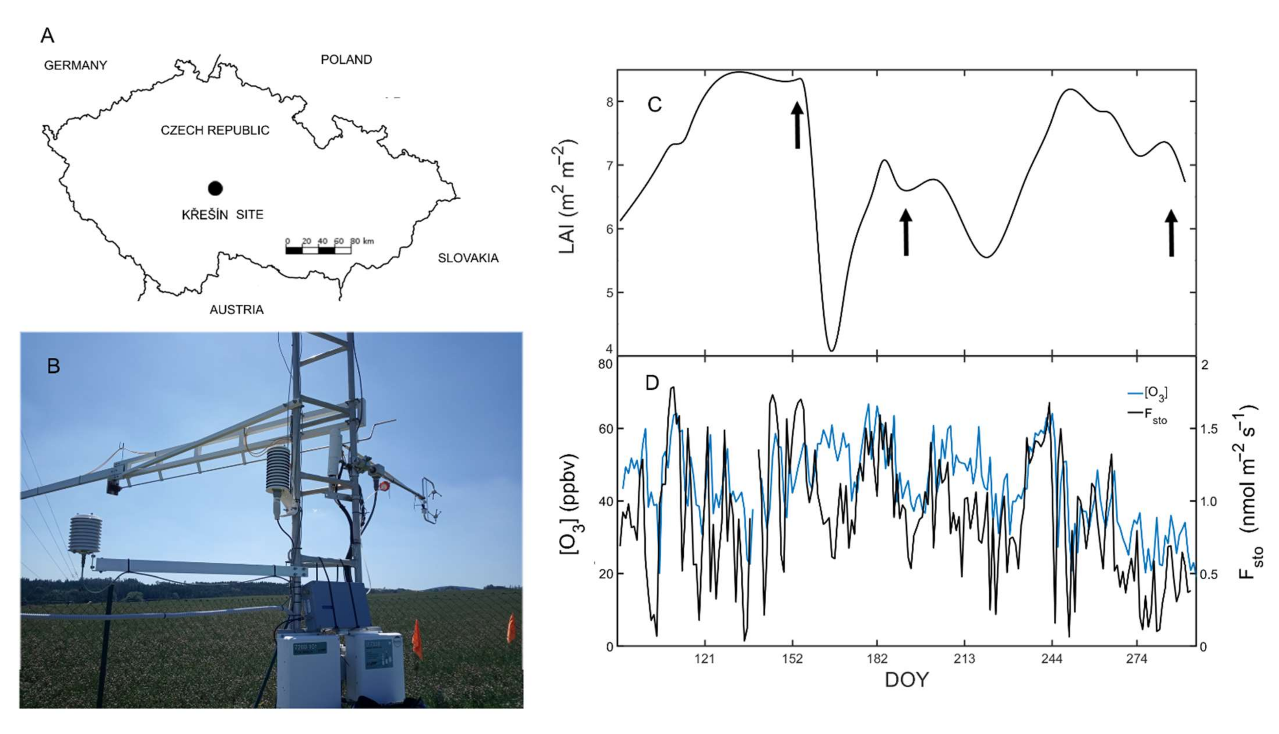
2.1. Experimental Site Description

The annual ryegrass–clover mixture (total area of 75 ha of which eddy covariance footprint area is 20 ha) is situated on arable land in close proximity to the atmospheric station, Křešín u Pacova in the Czech Republic (N 49°35′, E 15°05′, 534 m a.s.l.). The atmospheric station is equipped for the measurement of greenhouse gases, selected air pollutants, and basic meteorological parameters [38] and forms a part of European infrastructure networks ICOS [39], GMOS [40], and ACTRIS [41].

The vegetation mixture was established in spring 2018 by sowing spring barley (Hordeum vulgare), garden pea (Pisum sativum), red clover (Trifolium pratense), and perennial ryegrass (Lolium perenne). The seed mixture consisted of 75 kg spring barley, 150 kg pea, 1 kg ryegrass and 18 kg clover sown per hectare. Fertilization (200 kg per hectare) with a mixture of ammonium nitrate and limestone (27% nitrogen) was applied five days after sowing. The legume-cereal mixture was harvested in July 2018 and the clover was harvested in October 2018. In 2019, the year of study, the growth of the original understory with dominating T. pratense and L. perenne continued.

The ryegrass–clover mixture was cut three times during the investigated vegetation season (10 June, 23 July and 21 October 2019). The total harvested dry matter biomass was 8.27, 3.30, and 1.82 tons per hectare, respectively. Leaf area index (LAI) reached maximum values of 8.5, 7.0 and 8.0 m² m⁻² before the first, second and third cut, respectively, and rapidly decreased at the beginning of September in relation with leaf senescence (Figure 1C). The LAI was estimated from a time series of the normalized difference vegetation index (NDVI), applying the equation validated for erectophile–planophile canopies [42]. NDVI was computed from red and near-infrared bands using the Google Earth Engine built-in function using Sentinel-2 MSI: MultiSpectral Instrument, Level-2A (surface reflectance) product with a spatial resolution of 10 m × 10 m [43]. The area is characterized by a long-term (2013–2019) annual mean temperature of 8.2 °C and 620 mm of precipitation. Generally, the highest precipitation occurs in July 2019, with an average of 71 mm. February is the driest month, with 23 mm of precipitation. Usually, July is the warmest month of the year, with an average temperature of 17.8 °C, while the lowest average temperatures occur in January, with −2.1 °C. Detailed seasonal courses of selected microclimatic variables during the year 2019, the year of study, are shown in Figure 2 and presented in the Results, Section 3.1.

2.2. Measurement of Microclimatic Parameters

Air temperature (T_a) and relative air humidity (RH) were measured 2 m above the soil surface using an EMS33 Rotro^® sensor (EMS, Brno, Czech Republic). Vapour pressure deficit (VPD) was calculated based on T_a and RH values [44]. Radiation sensors EMS12 (EMS, Brno, Czech Republic) and CNR4 (Kipp & Zonen, Delft, The Netherlands) were used to measure the intensity of incoming photosynthetically active radiation (PAR) and global radiation (R_g), respectively. A tipping bucket rain gauge, Model 52202 (R.M. Young Company, Traverse City, MI, USA) was used to measure precipitation. Soil water content (SWC) in a depth of 30 cm was measured by a water content reflectometer, Model CS616L (Campbell Scientific, Logan, UT, USA). The signals from all sensors were recorded at 30 s intervals and stored as 30-min averages in the data logger RailBox V32P4 DX (EMS, Brno, Czech Republic).

2.3. Eddy Covariance Flux Measurements

Measurement of CO₂, H₂O, and O₃ fluxes between the ecosystem and the atmosphere was performed by the eddy covariance technique. The sensors, following the recommendations of pan-European infrastructure for flux measurements (ICOS), were mounted on a micrometeorological tower at 2.6 m above the soil surface, including a Gill R3^® ultrasonic anemometer (Gill Instruments, Hampshire, UK), LI-7200 CO₂/H₂O gas analyser (LI-COR Biosciences, Lincoln, NE, USA), and FOS fast chemiluminescence O₃ detector (Sextant Technologies, Wellington, New Zeland). The PTFE inlet line (length 1.2 m; ID 4 mm) was equipped with a PTFE filter (porosity of 5 μm) to prevent dust and particles from entering. Regular re-calibration of [O₃] was performed by a slow-response O₃ analyser APOA 370 (Horiba, Kyoto, Japan), which was regularly calibrated by an O₃ calibration source (model 306; 2B Technologies, Boulder, CO, USA). The ratio method [45] was applied to obtain 10 Hz [O₃].

All high-frequency eddy covariance data were processed by EddyPro 7.0.6 software and 30-min averaged flux values were calculated as:

$$F=\overline{w\prime c\prime }$$

(1)

where F is the flux, measured in nmol m⁻² s⁻¹, w represents the vertical wind component (m s⁻¹), c is the measured concentration of a given substance (CO₂, H₂O, O₃), prime (′) refers to the fluctuations and the overbar indicates an average over the time period. Averaged flux values were evaluated for data quality. During most of the day-time, the footprint was located within the crop field. If not, the data were discarded.

For the flux calculation, the OpenEddy 0.0.0.9004 software [46] was used for thorough quality-checking, applying the standardized methodology similar to Mauder et al. [47]. The screening of the data included checking the plausible range, testing for integral turbulence characteristics [48], fetch filtering accepting only the data when more than 70% of the measured flux originated from the target area, and iterative low frequency spike removal [49]. These data quality tests are used by default within the ICOS community. The REddyPro software [50] was used to additionally filter half-hourly periods with insufficient turbulent mixing (i.e., u_* filtering), gap-fill NEP (CO₂ flux) data, and partition NEP into GPP and ecosystem respiration R_eco. For the u_* filtering of NEP, the moving point method was applied [49,51]. To gapfill the missing NEP, the marginal distribution sampling [51] was used, where fluxes within a certain time window are binned to represent measurements during similar meteorological conditions [50]. Estimates of GPP were derived as the residual of R_eco and NEP within so-called nighttime partitioning [51]. The methods used to perform each of these steps are discussed in detail in Wutzler et al. [50].

2.4. Modelling of Stomatal O₃ Flux

Stomatal (F_sto) and total O₃ flux (F_tot) were modeled from the aerodynamic (r_a) and canopy (r_c) resistances, and the resistance of the leaf boundary layer (r_b) [37]. F_tot and F_sto (nmol m⁻² s⁻¹) were calculated as:

F_tot = V_d × c

(2)

F_sto = V_dsto × c

(3)

where c is [O₃] in a reference height of 2.6 m (ppbv), V_d is a dry deposition velocity (1/(r_a + r_b + r_c); m s⁻¹), and V_dsto is the deposition velocity to stomata and mesophyll (m s⁻¹).

The model was enhanced to include stability corrections and distinguish between stable, neutral and unstable atmospheric conditions within the resistance r_a [52]. The degree of atmospheric stability was further incorporated into the model. See the complete set of equations used and the detailed description of the entire model in the Supplementary Materials.

2.5. Modelling and Statistical Analyses

The effects of [O₃] and F_sto on NEP were modelled by linear mixed-effects models using the lmer function from the ‘lme4’ package [53] in R 4.1.0 [54]. Half-hour eddy covariance and microclimatic data of the daytime period (06:00–18:30), when R_g ≥ 10 W m⁻² and the photosynthesis was thus sufficiently developed, were used for further analyses. The GPP together with [O₃] or F_sto were used as NEP predictors. We assumed pre-industrial and future [O₃] of 12 and 60 ppbv, respectively, as reported by Cooper et al. [3] and Dentener et al. [4]. The corresponding F_sto values are 0.038 and 1.438 nmol m⁻² s⁻¹ for pre-industrial and future conditions, respectively. Relationships between predictors, their interactions and NEP were tested for linearity. Only significant linear correlations were found. Predictors were included in the model in order to minimize AIC (Akaike information criterion) and p-values. Day of observation was used as a random factor. Package ‘merTools’ [55] provides methods for extracting results from mixed-effect model objects fit with the ‘lme4’ package. We used the function to predict the interval from this package to obtain the NEP and [O₃] or F_sto relationship with its prediction bounds.

3. Results

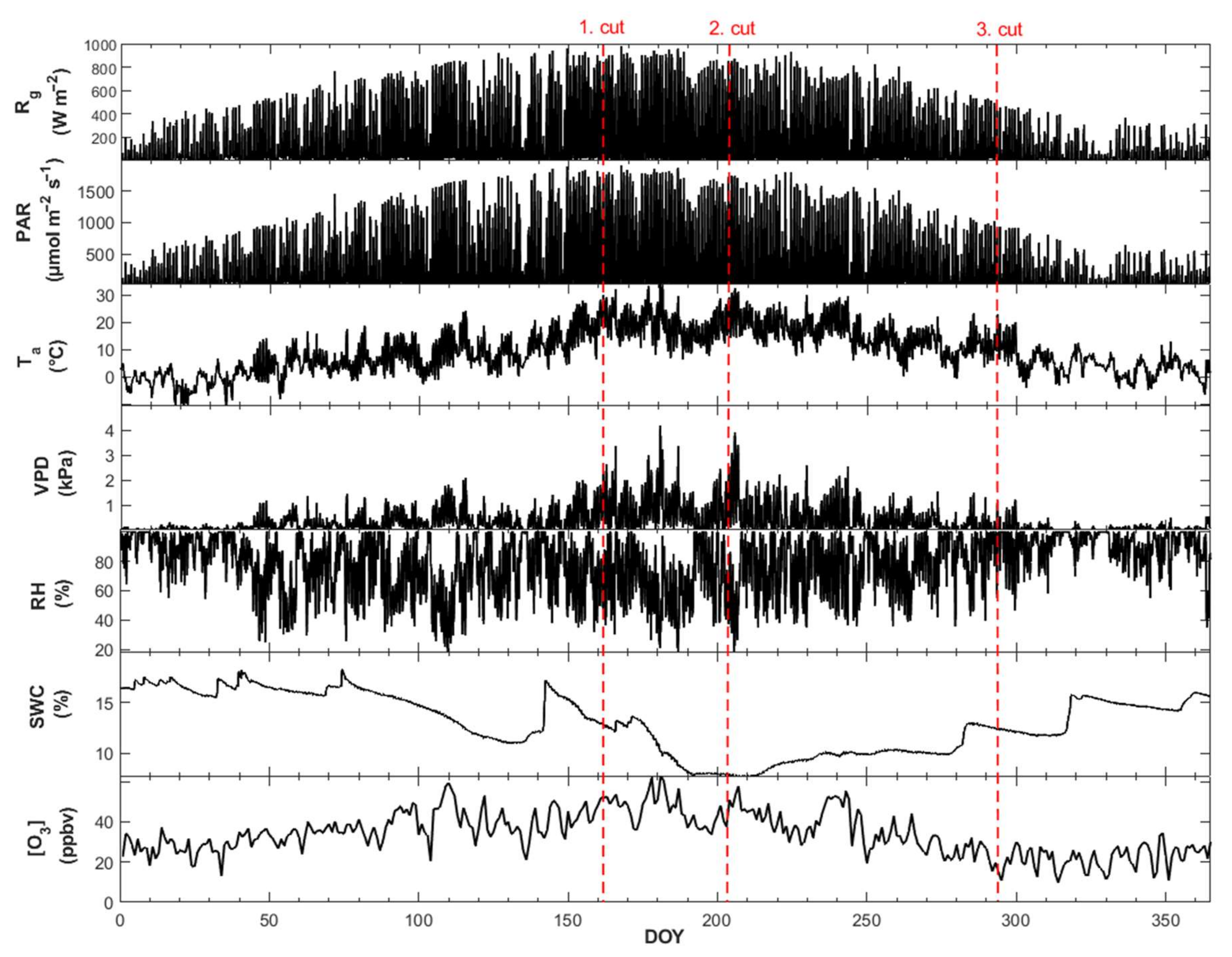
3.1. Microclimatic Growth Conditions

During the period of measurement (1 April–21 October 2019), the mean T_a was 14.5 °C, RH was 72.9%, and SWC was 11.2%. Values of R_g, PAR, T_a, and VPD had typical annual courses, with values highest during summer months (June–August) (Figure 2). The highest values of soil water content (15.0–17.0%) were observed at the beginning of the growing season (April) and the lowest (7.0%) in July.

The onset of the growing season was characterized by high values of mean daylight [O₃] ranging between 20 (overcast, rainy days) and 60 ppbv (clear sky conditions) before the first cut of the grass mixture. During the investigated period, the maximum and minimum values of 30-min averages of [O₃] were 63 and 27 ppbv, which occurred in late June and late October, respectively (Figure 1D and Figure 2).

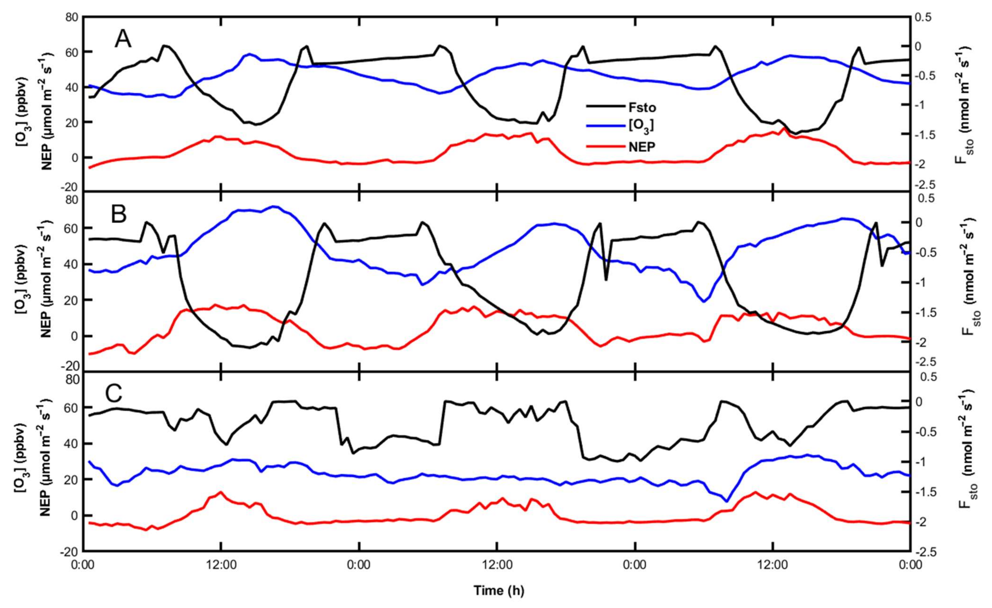
3.2. Daily Courses of [O₃], F_sto and NEP

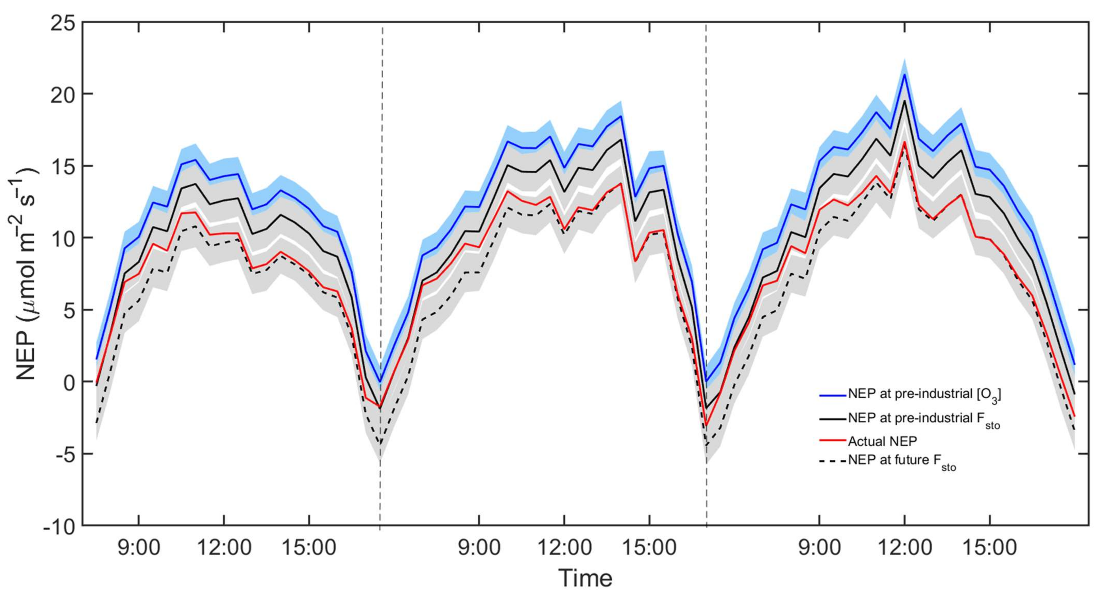
Detailed diurnal changes in [O₃], F_sto and NEP during three representative days of spring, summer and autumn seasons are shown in Figure 3. The highest [O₃] values occurred in the summer season, while the lowest values of [O₃] were observed in autumn (Figure 3). In addition, the differences between daily maxima and night minima were negligible at the end of the vegetation season. Similarly, F_sto showed typical daily courses characterized by their maximal and minimal values in clear sky summer days; however, they kept more or less constant during cloudy autumn days characterized by low values of VPD. Daily maxima of F_sto were up to −1.5 and −2.0 nmol m⁻² s⁻¹ in spring and summer (Figure 3A,B), respectively, but only up to −0.5 nmol m⁻² s⁻¹ in autumn (Figure 3C). [O₃] and F_sto values do not necessarily correlate as shown in Figure 1D; such inconsistencies likely correspond to stomatal closure preventing the diffusion of O₃ into the inner tissues.

The highest daily NEP values, up to 36.6 μmol m⁻² s⁻¹, were observed in the spring (Figure 3), when PAR, R_g, and SWC are the highest (Figure 2). However, the daily maxima of NEP only amounted to 25.4 μmol m⁻² s⁻¹ in the summer, when low SWC values were noticed (DOY 247), indicating a stomatal limitation on CO₂ diffusion into the leaves. Nocturnal NEP values, reflecting net ecosystem respiration, were up to −12.8 μmol m⁻² s⁻¹ in summer, the season characterized by high temperatures over the night (up to 19 °C). In contrast, the lowest night-time NEP values (−7.4 μmol m⁻² s⁻¹) were found in autumn (Figure 3C).

3.3. NEP Modelling

The linear mixed-effects models were used to determine the relations between NEP and its predictors (irradiance, temperature, VPD, etc.) along with [O₃] and F_sto. The NEP data, as half-hour averages, were modelled for the daytime period (06:00–18:30), when R_g ≥ 10 W m⁻² and air turbulence was always sufficiently developed. In addition, the model was used to calculate NEP based on fixed values of gross primary production (GPP) during the investigated growing period (Figure S1A,B). The performance of the model is shown in

Table 1. Outputs of linear mixed-effects model predicting values of net ecosystem production (NEP) based on [O₃] and F_sto for fixed gross primary productivity (GPP) values. Linear predictors and linear interaction statistics are shown as t-values and p-values, whereas statistics of predictors used as smooth terms are shown as p-values. × indicates interaction. The parametric estimate is similar to the slope of regression analysis, representing the increase of predictor (if positive) values due to [O₃] or F_sto. For example, the parametric estimate for F_sto is –1.767, indicating negative relationship of F_sto on NEP. The other parameters are statistics (p, t-value). R² (Marginal) = 0.905 for model F_sto and R² (Marginal) = 0.920 for model [O₃], n = 4398. [O₃]: ozone concentration; F_sto: stomatal ozone flux. **: p < 0.001.

Model	Predictor/ Interaction	Parametric Estimate	Goodness of Fit Std. Error	t-Value	Statistics p-Value
Model Fsto	Fsto	−1.767	0.069	−25.45	2.00·10−16 **
	GPP	1.055	0.005	223.95	2.00·10−16 **
	GPP × Fsto	−0.022	0.004	−6.18	7.18·10−16 **
Model [O3]	[O3]	−0.076	0.002	−31.90	2.00·10−16 **
	GPP	1.067	0.007	161.06	2.00·10−16 **
	[O3] × GPP	−0.002	0.000	−12.54	2.00·10−16 **

.

Diurnal courses of NEP were modelled for the whole growing season, from which an example of three consecutive days (06:00–18:30) is shown in Figure 4. Comparing to current O₃ conditions, the model predicts an increase in NEP when it is parametrized with low, pre-industrial [O₃] (12 ppbv) or F_sto (0.038 nmol m⁻² s⁻¹), while NEP decreases when the model is parametrized with high (future) [O₃] (60 ppbv) or F_sto (1.438 nmol m⁻² s⁻¹). The differences between NEP values measured by eddy covariance and those modelled by linear mixed-effects models at actual [O₃] and F_sto were less than 1% (

Table 2. Values of ozone concentration ([O₃], ppbv), stomatal ozone flux (F_sto, nmol m⁻² s⁻¹), and monthly sum of net ecosystem production (NEP, mol m⁻²) predicted by a linear mixed-effects (LM) model for the conditions of low and high [O₃] and F_sto during the individual months of the growing season from 1 April to 21 October 2019. Δ represents the percentage difference of predicted NEP to actual NEP measured by an eddy covariance system. Symbols ↑ represent increases in NEP at low [O₃] (12 ppbv) and/or F_sto (0.038 nmol m⁻² s⁻¹). Symbols ↓ represent decreases in NEP induced by high [O₃] (60 ppbv) and/or F_sto (1.438 nmol m⁻² s⁻¹).

Month	NEP (mol m−2)		ΔNEP (%)		ΔNEP (%)
	EC	LM	Low [O3]	High [O3]	Low Fsto	High Fsto
April	10.729	10.708	↑ 28.1	↓ 13.9	↑ 16.6	↓ 12.1
May	15.769	15.764	↑ 21.1	↓ 13.3	↑ 13.1	↓ 8.1
June	10.017	10.050	↑ 36.2	↓ 7.9	↑ 23.5	↓ 6.9
July	7.967	7.982	↑ 38.8	↓ 18.2	↑ 26.2	↓ 13.8
August	9.256	9.276	↑ 33.5	↓ 16.2	↑ 21.0	↓ 13.0
September	9.962	9.968	↑ 23.7	↓ 28.7	↑ 15.9	↓ 7.0
October	2.671	2.670	↑ 30.2	↓ 86.6	↑ 17.1	↓ 61.0

). Both models (based on [O₃] and/or F_sto) confirmed a substantial reduction in NEP induced by O₃ over the whole season when measured NEP values are compared to those modelled for the pre-industrial O₃ conditions. The estimated reduction of NEP ranges between 21.1% (May) and 38.8% (July) and between 13.1% and 26.2% when models based on [O₃] and F_sto are applied, respectively.

To predict the future O₃-induced changes in NEP, [O₃] and F_sto of 60 ppbv and 1.438 nmol m⁻² s⁻¹) were applied in the model. Although the largest percentage decreases in NEP at high O₃ conditions were found in October, the effect is comparatively lower due to a small total carbon uptake at the end of the growing season. In contrast, the largest absolute reduction in NEP occurred in June. Noticeably, reductions predicted by the F_sto-based model were lower as compared to those predicted by the [O₃]-based model over the entire growing season (Table 2).

Finally, values of a cumulative NEP (NEP_cumul), derived from the diurnal courses over the entire growing season, are shown in Figure 5. Values of NEP_cumul were calculated as sums of daily NEP totals directly estimated by eddy covariance or modelled for the pre-industrial O₃ conditions from the beginning of the vegetation season (1 April 2019). In total, approximately 8.1 t of carbon was fixed per hectare over the growing season, when calculated from NEP over day hours (6:00–18:30), when the eddy covariance technique is generally more reliable. Additionally, the yield after the 1st, 2nd, and 3rd cut was 16.57, 6.7 and 3.65 t ha⁻¹ in the form of green fodder, which corresponded to 8.27, 3.3 and 1.82 t ha⁻¹ when dried. That corresponds to approximately 60.5% of C in dried biomass, when night-time respiration is not taken into account. Comparing to NEP_cumul measured by eddy covariance at actual O₃ conditions, the model parametrized by low, pre-industrial [O₃] (12 ppbv) revealed higher values of NEP_cumul, as much as 29.7%; however, it was only 13.5% when the model based on pre-industrial F_sto (0.038 nmol m⁻² s⁻¹) was used.

4. Discussion

Previous studies have shown that tropospheric O₃ reduces carbon uptake in the forest [56] and grassland ecosystems [27,28]. Here, we aimed to quantify reductions in NEP of a managed ryegrass–clover mixture caused by current O₃ conditions and to predict these reductions under the O₃ conditions expected in the future. Indeed, we found an annual O₃-induced reduction of NEP by 13.5–29.7% when compared to low pre-industrial O₃ conditions, depending on the construction of the predictive linear mixed-effects model. Accordingly, the accuracy of the models based on F_sto and tropospheric [O₃] was compared. Our findings show that F_sto is a better predictor of O₃ deposition and NEP decrease as compared to [O₃] (Figure 1D). High [O₃] does not necessarily result in high penetration of O₃ into plant tissues (F_sto; Figure 1D) due to closure of stomatal aperture over the noon hours, when [O₃] usually peaks [32]. Prediction of negative O₃ effects may be thus overestimated in [O₃]-based models. On the contrary, even low [O₃] of 3–5 ppbv may provide sufficient F_sto inducing injuries of photosynthetic apparatus when stomata remain open [57].

Previous studies at a range of ecosystems found that microclimatic conditions at cloudy or semi-cloudy skies including optimum light intensity, T_a and/or low VPD lead to a substantial stomatal openness and consequently high F_sto [32,58,59]. Vice versa, high T_a, light intensities, and VPD, together with low SWC, result in reduced stomatal conductance and F_sto [60,61]. In accordance, we observed low F_sto during the summer season (June–August) when VPD, T_a, and light intensities are the highest together with high [O₃] and low SWC (Figure 2 and Figure 3). On the contrary, F_sto was highest in spring and autumn when VPD, T_a, R_g and PAR were lower, and SWC had increased and [O₃] remained lower than in summer. Such mechanism is likely to have been responsible for the relatively low stomatal conductance to O₃ diffusion and low O₃-induced injuries in arid and hot South-European ecosystems as compared to high injuries of photosynthetic activity, plant growth and productivity observed in cold and wet North-European ecosystems [13,62]. However, severe drought periods can induce the hydro passive opening of the guard cells in Angiosperms and Gymnosperms [63], leading consequently to exacerbated O₃ damage [64]. Moreover, actual microclimatic conditions, particularly the seasonal course of VPD, have a strong effect on phenology and overall productivity of terrestrial ecosystems [65].

Tropospheric [O₃] has a typical seasonal course. In western Europe, [O₃] reaches its maximum in Spring, while, in Central and Eastern Europe, [O₃] is maximal in Summer [66]. We confirm the broad Summer maximum of [O₃], which was, however, not followed by the biggest NEP decline. Such a paradox is the result of low soil moisture (SWC) leading to a low stomatal conductivity and F_sto. We found the highest O₃-induced reduction of NEP in the Spring to Summer transition (June–July) compared to predicted values of NEP at pre-industrial [O₃] (Figure 4 and Table 2), i.e., the period of convenient conditions for stomatal openness and high F_sto (Figure 1D). This finding shows a strong interactive effect of [O₃] and microclimatic conditions on plant injuries [2].

We estimated the reduction of NEP, relative to pre-industrial conditions, to be between 13.1% in May and 26.2% in July. Previous studies indicated that the O₃-induced decrease in NEP is associated with impaired photosynthetic CO₂ uptake, root respiration, and stomatal conductance as well as premature senescence of plants [34]. Such changes may further lead to a reduced biomass accumulation, yield quantity and crop quality [67]. Reduced photosynthesis is particularly associated with oxidized fatty acids of bio-membranes, enhanced production of reactive oxygen species (ROS) resulting in the degradation of chloroplasts, photosynthetic pigments and morphological changes of mesophylls [12]. In a meta-analysis of O₃-induced effects on crops, Feng and Kobayashi [68] compared crop responses to [O₃] ranging between <26 and 75 ppbv. For wheat, a reduction of 9.7% in grain yield is observed in plants treated at 31–50 ppbv (current [O₃]) as compared to those treated at [O₃] below 26 ppbv. Further increase of [O₃] to 51–75 ppbv leads to an additional decrease of yield by 10% when compared to [O₃] of 31–50 ppbv. A modelling study covering Euro-Mediterranean vegetation revealed an O₃-induced reduction of GPP of 22% and LAI of 15–20% [69], with the greatest reduction in summer, along with the peak of tropospheric [O₃]. That is in line with our observation when the largest reduction of NEP in July was found.

There is a huge variety in plant sensitivity to [O₃]. Such variability is likely to be the consequence of the capacity of the detoxification processes that are genetically based [70]. Studying Trifolium and Lolium species, Hayes et al. [22] reported a decrease of biomass by 33% in T. repens due to O₃ exposure, but no effect on L. perenne grown either in a mixture or monoculture (no change of canopy structure was observed when the species were grown in monoculture or mixture [22]. A mixture of T. pratense and Phleum pratense under elevated [O₃] showed similar results with a decrease in biomass yield of T. pratense [71]. That suggests higher capacity of L. perenne for O₃ removal and perhaps it out-competes T. repens in elevated [O₃], leading to changes in species composition when grown in mixtures. The possible unbalanced reduction has a significant effect on pasture communities, where those species are more-or-less co-dominant, because it allows invasion of other O₃ tolerant species. In addition, a reduction of stolon biomass has been reported in T. pratense, which results in a higher reduction in later grassland cuttings due to a carry-over effect. New leaves are produced from nodes of stolons, therefore the ability of the plant to spread and build up new biomass is reduced [22]. A further reduction has been observed due to a decrease of nodulation in T. repens when grown in monoculture [72] and mixture [73]. That further affects N-fixing capacity and diversion of assimilates away from the energetically costly process of N-fixation and nodule growth. Therefore, we assume that in our experimental site, L. perenne partially balanced the larger reduction of T. pratense biomass.

A broad range of field studies has shown that precise estimation of F_sto is crucial for calculation of ozone deposition velocity, and thus of F_sto. Therefore, precise estimation of F_sto is needed. In our case, the model error is below 1%, which is far below the varying differences in O₃ deposition rates of 13% found by Otu-Larbi et al. [74]. However, it should be noted that our model predicts pre-industrial NEP based on fixed value of [O₃] and F_sto over the day, which has no effect on the prediction due to the linearity of the model. Nevertheless, having diurnal variation in those variables will be at least logically more relevant, although modelling the shape of the diurnal profile during the pre-industrial era will be difficult due to the lack of diurnal observations in the past. We found that the model based on [O₃] shows the reduction in cumulative measured NEP at low, pre-industrial [O₃] by as much as 29.7% against a reduction of 13.5% with the model based on F_sto (Figure 5). In line with our finding, F_sto is recommended to be applied for modelling studies and estimations of vegetation damage [75]. Nevertheless, European legislation is still based on [O₃] instead of F_sto (European Council Directive 2008/50/EC). Moreover, only [O₃] is monitored at most European localities [76]. Therefore, studies comparing both approaches are needed.

5. Conclusions

We quantified the reductions in NEP of a managed ryegrass–clover mixture caused by current O₃ conditions compared to pre-industrial O₃ conditions and we predicted these reductions under expected future O₃ conditions. Reductions of NEP were estimated by a linear mixed-effects model based on O₃ concentration ([O₃]) and stomatal O₃ flux (F_sto). We found the F_sto-based model more precise, showing high F_sto and, consequently, substantial NEP reduction even during low [O₃] periods. On the contrary, the broad summer maximum of [O₃] is not followed by the biggest NEP decline, due to low soil water content leading to a low stomatal conductivity and F_sto. Compared to the lower pre-industrial O₃ conditions, current levels of O₃ result in a reduction of cumulative NEP over the entire growing season of up to 29.7 and 13.5% when the [O₃]-based and F_sto-based model is applied, respectively. The intra-annual reduction varies between 13.1% in May and 26.2% in July in the F_sto model. These findings indicate the importance of F_sto and its inclusion into the models estimating O₃ effects on terrestrial vegetation.

References

1. Monks, P.S.; Granier, C.; Fuzzi, S.; Stohl, A.; Williams, M.L.; Akimoto, H.; Amann, M.; Baklanov, A.; Baltensperger, U.; Bey, I. Atmospheric composition change–global and regional air quality. Atmos. Environ. 2009, 43, 5268–5350. [Google Scholar] [CrossRef] [Green Version]
2. Juráň, S.; Grace, J.; Urban, O. Temporal changes in ozone concentrations and their impact on vegetation. Atmosphere 2021, 12, 82. [Google Scholar] [CrossRef]
3. Cooper, O.R.; Parrish, D.; Ziemke, J.; Balashov, N.; Cupeiro, M.; Galbally, I.; Gilge, S.; Horowitz, L.; Jensen, N.; Lamarque, J.-F. Global distribution and trends of tropospheric ozone: An observation-based reviewGlobal distribution and trends of tropospheric ozone. Elementa 2014, 2, 000029. [Google Scholar] [CrossRef]
4. Dentener, F.; Stevenson, D.; Ellingsen, K.; van Noije, T.; Schultz, M.; Amann, M.; Atherton, C.; Bell, N.; Bergmann, D.; Bey, I. The global atmospheric environment for the next generation. Environ. Sci. Technol. 2006, 40, 3586–3594. [Google Scholar] [CrossRef] [PubMed] [Green Version]
5. Granier, C.; Bessagnet, B.; Bond, T.; D’Angiola, A.; van Der Gon, H.D.; Frost, G.J.; Heil, A.; Kaiser, J.W.; Kinne, S.; Klimont, Z. Evolution of anthropogenic and biomass burning emissions of air pollutants at global and regional scales during the 1980–2010 period. Clim. Change 2011, 109, 163–190. [Google Scholar] [CrossRef]
6. Agyei, T.; Juráň, S.; Ofori-Amanfo, K.K.; Šigut, L.; Urban, O.; Marek, M.V. The impact of drought on total ozone flux in a mountain Norway spruce forest. J. For. Sci. 2020, 66, 278–280. [Google Scholar] [CrossRef]
7. Hůnová, I.; Livorová, H.; Ostatnická, J. Potential ambient ozone impact on ecosystems in the Czech Republic as indicated by exposure index AOT40. Eco. Indic. 2003, 3, 35–47. [Google Scholar] [CrossRef]
8. Tai, A.P.; Martin, M.V.; Heald, C.L. Threat to future global food security from climate change and ozone air pollution. Nat. Clim. Change 2014, 4, 817–821. [Google Scholar] [CrossRef] [Green Version]
9. Mills, G.; Hayes, F.; Simpson, D.; Emberson, L.; Norris, D.; Harmens, H.; Bueker, P. Evidence of widespread effects of ozone on crops and (semi-) natural vegetation in Europe (1990–2006) in relation to AOT40-and flux-based risk maps. Glob. Change Biol. 2011, 17, 592–613. [Google Scholar] [CrossRef] [Green Version]
10. Mills, G.; Hayes, F.; Jones, M.; Cinderby, S. Identifying ozone-sensitive communities of (semi-) natural vegetation suitable for mapping exceedance of critical levels. Environ. Pollut. 2007, 146, 736–743. [Google Scholar] [CrossRef]
11. Gandin, A.; Davrinche, A.; Jolivet, Y. Deciphering the main determinants of O3 tolerance in Euramerican poplar genotypes. Sci. Total Environ. 2019, 656, 681–690. [Google Scholar] [CrossRef] [PubMed]
12. Zapletal, M.; Juran, S.; Krpes, V.; Michna, K.; Cudlin, P.; Edwards, M. Effect of ozone flux on selected structural and antioxidant characteristics of a mountain norway spruce forest. Balt. For. 2018, 24, 261–267. [Google Scholar]
13. Wittig, V.E.; Ainsworth, E.A.; Naidu, S.L.; Karnosky, D.F.; Long, S.P. Quantifying the impact of current and future tropospheric ozone on tree biomass, growth, physiology and biochemistry: A quantitative meta-analysis. Glob. Change Biol. 2009, 15, 396–424. [Google Scholar] [CrossRef]
14. Goumenaki, E.; Taybi, T.; Borland, A.; Barnes, J. Mechanisms underlying the impacts of ozone on photosynthetic performance. Environ. Exp. Bot. 2010, 69, 259–266. [Google Scholar] [CrossRef]
15. Hoshika, Y.; Watanabe, M.; Inada, N.; Koike, T. Model-based analysis of avoidance of ozone stress by stomatal closure in Siebold’s beech (Fagus crenata). Ann. Bot. 2013, 112, 1149–1158. [Google Scholar] [CrossRef] [PubMed]
16. Di Baccio, D.; Castagna, A.; Paoletti, E.; Sebastiani, L.; Ranieri, A. Could the differences in O3 sensitivity between two poplar clones be related to a difference in antioxidant defense and secondary metabolic response to O3 influx? Tree Physiol. 2008, 28, 1761–1772. [Google Scholar] [CrossRef] [PubMed] [Green Version]
17. Grantz, D.; Gunn, S.; Vu, H.B. O3 impacts on plant development: A meta-analysis of root/shoot allocation and growth. Plant Cell Environ. 2006, 29, 1193–1209. [Google Scholar] [CrossRef]
18. Rodwell, J. British Plant Communities: Grasslands and Montane Communities; Cambridge University Press: Cambridge, UK, 1992. [Google Scholar]
19. Veen, P.; Jefferson, R.; De Smidt, J.; van der Straaten, J. Grasslands in Europe: Of High Nature Value; KNNV Publishing: Zeist, The Netherlands, 2009. [Google Scholar]
20. Wilbourn, S.; Davison, A.; Ollerenshaw, J. The use of an unenclosed field fumigation system to determine the effects of elevated ozone on a grass–clover mixture. New Phytol. 1995, 129, 23–32. [Google Scholar] [CrossRef]
21. Nussbaum, S.; Bungener, P.; Geissmann, M.; Fuhrer, J. Plant–plant interactions and soil moisture might be important in determining ozone impacts on grasslands. New Phytol. 2000, 147, 327–335. [Google Scholar] [CrossRef]
22. Hayes, F.; Mills, G.; Ashmore, M. Effects of ozone on inter-and intra-species competition and photosynthesis in mesocosms of Lolium perenne and Trifolium repens. Environ. Pollut. 2009, 157, 208–214. [Google Scholar] [CrossRef]
23. Evans, P.A.; Ashmore, M. The effects of ambient air on a semi-natural grassland community. Agric. Ecosyst. Environ. 1992, 38, 91–97. [Google Scholar] [CrossRef]
24. Ren, W.; Tian, H.; Tao, B.; Chappelka, A.; Sun, G.; Lu, C.; Liu, M.; Chen, G.; Xu, X. Impacts of tropospheric ozone and climate change on net primary productivity and net carbon exchange of China's forest ecosystems. Glob. Ecol. Biogeogr. 2011, 20, 391–406. [Google Scholar] [CrossRef]
25. Oliver, R.J.; Mercado, L.M.; Sitch, S.; Simpson, D.; Medlyn, B.E.; Lin, Y.-S.; Folberth, G.A. Large but decreasing effect of ozone on the European carbon sink. Biogeosciences 2018, 15, 4245–4269. [Google Scholar] [CrossRef] [Green Version]
26. Felzer, B.; Kicklighter, D.; Melillo, J.; Wang, C.; Zhuang, Q.; Prinn, R. Effects of ozone on net primary production and carbon sequestration in the conterminous United States using a biogeochemistry model. Tellus B Chem. Phys. Meteorol. 2004, 56, 230–248. [Google Scholar] [CrossRef]
27. Ren, W.; Tian, H.; Liu, M.; Zhang, C.; Chen, G.; Pan, S.; Felzer, B.; Xu, X. Effects of tropospheric ozone pollution on net primary productivity and carbon storage in terrestrial ecosystems of China. J. Geophys. Res. Atmos. 2007, 112, D22S09. [Google Scholar] [CrossRef]
28. Felzer, B.S.; Cronin, T.; Reilly, J.M.; Melillo, J.M.; Wang, X. Impacts of ozone on trees and crops. Comptes Rendus Geosci. 2007, 339, 784–798. [Google Scholar] [CrossRef] [Green Version]
29. Cailleret, M.; Ferretti, M.; Gessler, A.; Rigling, A.; Schaub, M. Ozone effects on European forest growth—Towards an integrative approach. J. Ecol. 2018, 106, 1377–1389. [Google Scholar] [CrossRef]
30. Nussbaum, S.; Remund, J.; Rihm, B.; Mieglitz, K.; Gurtz, J.; Fuhrer, J. High-resolution spatial analysis of stomatal ozone uptake in arable crops and pastures. Environ. Int. 2003, 29, 385–392. [Google Scholar] [CrossRef]
31. Hayes, F.; Wagg, S.; Mills, G.; Wilkinson, S.; Davies, W. Ozone effects in a drier climate: Implications for stomatal fluxes of reduced stomatal sensitivity to soil drying in a typical grassland species. Glob. Change Biol. 2012, 18, 948–959. [Google Scholar] [CrossRef] [Green Version]
32. Juráň, S.; Šigut, L.; Holub, P.; Fares, S.; Klem, K.; Grace, J.; Urban, O. Ozone flux and ozone deposition in a mountain spruce forest are modulated by sky conditions. Sci. Total Environ. 2019, 672, 296–304. [Google Scholar] [CrossRef]
33. Xu, J.; Zheng, Y.; He, Y.; Zhu, F.; Mai, B.; Wang, S.; Zhang, M.; Zhao, X.; Wang, L.; Xu, L.; et al. Estimating stomatal conductance and partitioning total ozone uptake over a winter wheat field. Atmos. Pollut. Res. 2019, 10, 904–912. [Google Scholar] [CrossRef]
34. Ainsworth, E.A.; Yendrek, C.R.; Sitch, S.; Collins, W.J.; Emberson, L.D. The effects of tropospheric ozone on net primary productivity and implications for climate change. Annu. Rev. Plant Biol. 2012, 63, 637–661. [Google Scholar] [CrossRef] [PubMed] [Green Version]
35. Wilkinson, S.; Mills, G.; Illidge, R.; Davies, W.J. How is ozone pollution reducing our food supply? J. Exp. Bot. 2012, 63, 527–536. [Google Scholar] [CrossRef]
36. Long, S.P. Virtual Special Issue on food security–greater than anticipated impacts of near-term global atmospheric change on rice and wheat. Glob. Change Biol. 2012, 18, 1489–1490. [Google Scholar] [CrossRef]
37. Emberson, L.; Ashmore, M.; Cambridge, H.; Simpson, D.; Tuovinen, J.-P. Modelling stomatal ozone flux across Europe. Environ. Pollut. 2000, 109, 403–413. [Google Scholar] [CrossRef]
38. Dvorská, A.; Sedlák, P.; Schwarz, J.; Fusek, M.; Hanuš, V.; Vodička, P.; Trusina, J. Atmospheric station Křešín u Pacova, Czech Republic–a Central European research infrastructure for studying greenhouse gases, aerosols and air quality. Adv. Sci. Res. 2015, 12, 79–83. [Google Scholar] [CrossRef] [Green Version]
39. Integrated Carbon Observation System Home Page. Available online: https://www.icos-cp.eu (accessed on 24 September 2021).
40. Global Mercury Observation System. Available online: http://www.gmos.eu (accessed on 27 September 2021).
41. Aerosol, Clouds, and Trace Gases Research Infrastructure Network. Available online: https://www.actris.eu (accessed on 25 September 2021).
42. Tan, C.-W.; Zhang, P.-P.; Zhou, X.-X.; Wang, Z.-X.; Xu, Z.-Q.; Mao, W.; Li, W.-X.; Huo, Z.-Y.; Guo, W.-S.; Yun, F. Quantitative monitoring of leaf area index in wheat of different plant types by integrating NDVI and Beer-Lambert law. Sci. Rep. 2020, 10, 929. [Google Scholar] [CrossRef] [PubMed]
43. Gorelick, N.; Hancher, M.; Dixon, M.; Ilyushchenko, S.; Thau, D.; Moore, R. Google Earth Engine: Planetary-scale geospatial analysis for everyone. Remote Sens. Environ. 2017, 202, 18–27. [Google Scholar] [CrossRef]
44. Buck, A.L. New equations for computing vapor pressure and enhancement factor. J. Appl. Meteorol. Climatol. 1981, 20, 1527–1532. [Google Scholar] [CrossRef] [Green Version]
45. Zhu, Z.; Zhao, F.; Voss, L.; Xu, L.; Sun, X.; Yu, G.; Meixner, F.X. The effects of different calibration and frequency response correction methods on eddy covariance ozone flux measured with a dry chemiluminescence analyzer. Agric. For. Meteorol. 2015, 213, 114–125. [Google Scholar] [CrossRef]
46. OpenEddy Software. Available online: https://github.com/lsigut/openeddy (accessed on 26 September 2021).
47. Mauder, M.; Cuntz, M.; Drüe, C.; Graf, A.; Rebmann, C.; Schmid, H.P.; Schmidt, M.; Steinbrecher, R. A strategy for quality and uncertainty assessment of long-term eddy-covariance measurements. Agric. For. Meteorol. 2013, 169, 122–135. [Google Scholar] [CrossRef]
48. Foken, T.; Wichura, B. Tools for quality assessment of surface-based flux measurements. Agric. For. Meteorol. 1996, 78, 83–105. [Google Scholar] [CrossRef]
49. Papale, D.; Reichstein, M.; Aubinet, M.; Canfora, E.; Bernhofer, C.; Kutsch, W.; Longdoz, B.; Rambal, S.; Valentini, R.; Vesala, T. Towards a standardized processing of Net Ecosystem Exchange measured with eddy covariance technique: Algorithms and uncertainty estimation. Biogeosciences 2006, 3, 571–583. [Google Scholar] [CrossRef] [Green Version]
50. Wutzler, T.; Lucas-Moffat, A.; Migliavacca, M.; Knauer, J.; Sickel, K.; Šigut, L.; Menzer, O.; Reichstein, M. Basic and extensible post-processing of eddy covariance flux data with REddyProc. Biogeosciences 2018, 15, 5015–5030. [Google Scholar] [CrossRef] [Green Version]
51. Reichstein, M.; Falge, E.; Baldocchi, D.; Papale, D.; Aubinet, M.; Berbigier, P.; Bernhofer, C.; Buchmann, N.; Gilmanov, T.; Granier, A. On the separation of net ecosystem exchange into assimilation and ecosystem respiration: Review and improved algorithm. Glob. Change Biol. 2005, 11, 1424–1439. [Google Scholar] [CrossRef]
52. Liu, S.; Lu, L.; Mao, D.; Jia, L. Evaluating parameterizations of aerodynamic resistance to heat transfer using field measurements. Hydrol. Earth Syst. Sci. 2007, 11, 769–783. [Google Scholar] [CrossRef] [Green Version]
53. Bates, D.; Mächler, M.; Bolker, B.; Walker, S. Fitting Linear Mixed-Effects Models Using lme4. J. Stat. Softw. 2015, 67, 1–48. [Google Scholar] [CrossRef]
54. R Core Team. R: A Language and Environment for Statistical Computing. 2013. Available online: https://www.R-project.org/ (accessed on 21 October 2021).
55. Knowles, J.; Frederick, C.; Whitworth, A. Tools for Analyzing Mixed Effect Regression Models; The Comprehensive R Archive Network (CRAN): Vienna, Austria, 2020. [Google Scholar]
56. Juráň, S.; Edwards-Jonášová, M.; Cudlín, P.; Zapletal, M.; Šigut, L.; Grace, J.; Urban, O. Prediction of ozone effects on net ecosystem production of Norway spruce forest. iForest Biogeosci. For. 2018, 11, 743. [Google Scholar] [CrossRef] [Green Version]
57. Hayes, F.; Mills, G.; Alonso, R.; González-Fernández, I.; Coyle, M.; Grünhage, L.; Gerosa, G.; Karlsson, P.E.; Marzuoli, R. A site-specific analysis of the implications of a changing ozone profile and climate for stomatal ozone fluxes in Europe. Water Air Soil Pollut. 2019, 230, 4. [Google Scholar] [CrossRef] [Green Version]
58. Hu, Y.; Zhao, P.; Niu, J.; Sun, Z.; Zhu, L.; Ni, G. Canopy stomatal uptake of NOX, SO2 and O3 by mature urban plantations based on sap flow measurement. Atmos. Environ. 2016, 125, 165–177. [Google Scholar] [CrossRef]
59. Hoshika, Y.; Fares, S.; Savi, F.; Gruening, C.; Goded, I.; De Marco, A.; Sicard, P.; Paoletti, E. Stomatal conductance models for ozone risk assessment at canopy level in two Mediterranean evergreen forests. Agric. For. Meteorol. 2017, 234, 212–221. [Google Scholar] [CrossRef]
60. Emberson, L.D.; Büker, P.; Ashmore, M.R. Assessing the risk caused by ground level ozone to European forest trees: A case study in pine, beech and oak across different climate regions. Environ. Pollut. 2007, 147, 454–466. [Google Scholar] [CrossRef] [PubMed]
61. Schneuwly, J.; Ammann, C. Large regional differences of soil water limitation effect on ozone induced yield loss for wheat and potato in Switzerland. Sci. Total Environ. 2020, 718, 135257. [Google Scholar] [CrossRef] [PubMed]
62. Otu-Larbi, F.; Conte, A.; Fares, S.; Wild, O.; Ashworth, K. Current and future impacts of drought and ozone stress on Northern Hemisphere forests. Glob. Change Biol. 2020, 26, 6218–6234. [Google Scholar] [CrossRef]
63. Franks, P.J.; Farquhar, G.D. The mechanical diversity of stomata and its significance in gas-exchange control. Plant Physiol. 2007, 143, 78–87. [Google Scholar] [CrossRef] [Green Version]
64. Hoshika, Y.; Omasa, K.; Paoletti, E. Both ozone exposure and soil water stress are able to induce stomatal sluggishness. Environ. Exp. Bot. 2013, 88, 19–23. [Google Scholar] [CrossRef]
65. Yang, X.; Wu, J.; Chen, X.; Ciais, P.; Maignan, F.; Yuan, W.; Piao, S.; Yang, S.; Gong, F.; Su, Y.; et al. A comprehensive framework for seasonal controls of leaf abscission and productivity in evergreen broadleaved tropical and subtropical forests. Innovation 2021, 2, 100154. [Google Scholar] [CrossRef]
66. Monks, P.S. A review of the observations and origins of the spring ozone maximum. Atmos. Environ. 2000, 34, 3545–3561. [Google Scholar] [CrossRef]
67. Emberson, L.D.; Pleijel, H.; Ainsworth, E.A.; van den Berg, M.; Ren, W.; Osborne, S.; Mills, G.; Pandey, D.; Dentener, F.; Büker, P. Ozone effects on crops and consideration in crop models. Eur. J. Agron. 2018, 100, 19–34. [Google Scholar] [CrossRef]
68. Feng, Z.; Kobayashi, K. Assessing the impacts of current and future concentrations of surface ozone on crop yield with meta-analysis. Atmos. Environ. 2009, 43, 1510–1519. [Google Scholar] [CrossRef]
69. Anav, A.; Menut, L.; Khvorostyanov, D.; Viovy, N. Impact of tropospheric ozone on the Euro-Mediterranean vegetation. Glob. Change Biol. 2011, 17, 2342–2359. [Google Scholar] [CrossRef]
70. Luwe, M.; Heber, U. Ozone detoxification in the apoplasm and symplasm of spinach, broad bean and beech leaves at ambient and elevated concentrations of ozone in air. Planta 1995, 197, 448–455. [Google Scholar] [CrossRef]
71. Kohut, R.J.; Laurence, J.A.; Amundson, R.G. Effects of Ozone and Sulfur Dioxide on Yield of Red Clover and Timothy. J. Environ. Qual. 1988, 17, 580–585. [Google Scholar] [CrossRef]
72. Hewitt, D.; Mills, G.; Hayes, F.; Wilkinson, S.; Davies, W. Highlighting the threat from current and near-future ozone pollution to clover in pasture. Environ. Pollut. 2014, 189, 111–117. [Google Scholar] [CrossRef] [Green Version]
73. Hewitt, D.; Mills, G.; Hayes, F.; Davies, W. The climate benefits of high-sugar grassland may be compromised by ozone pollution. Sci. Total Environ. 2016, 565, 95–104. [Google Scholar] [CrossRef]
74. Otu-Larbi, F.; Conte, A.; Fares, S.; Wild, O.; Ashworth, K. FORCAsT-gs: Importance of stomatal conductance parameterisation to estimated ozone deposition velocity. J. Adv. Model. Earth Syst. 2021, 33, e2021MS002581. [Google Scholar] [CrossRef]
75. Sicard, P.; De Marco, A.; Carrari, E.; Dalstein-Richier, L.; Hoshika, Y.; Badea, O.; Pitar, D.; Fares, S.; Conte, A.; Popa, I. Epidemiological derivation of flux-based critical levels for visible ozone injury in European forests. J. For. Res. 2020, 31, 1509–1519. [Google Scholar] [CrossRef]
76. Hůnová, I. Ambient air quality in the Czech Republic: Past and present. Atmosphere 2020, 11, 214. [Google Scholar] [CrossRef] [Green Version]
Figure 1. (A) Geographical location of the research area (total area of 75 ha), (B) the experimental research site, Křešín, showing a ryegrass–clover (Lolium perenne, Trifolium pratense) mixture and the eddy covariance system (footprint area of 20 ha), (C) leaf area index (LAI), and (D) daily averages (06:00–18:30) of O3 concentration [O3] and stomatal O3 flux (Fsto) over the growing season (1 April–21 October 2019). Black arrows indicate the three cuttings of the ryegrass–clover mixture.
Atmosphere 12 01629 g001
Figure 2. Annual microclimatic conditions at Křešín experimental research site during the year of study, 2019: Rg—global radiation, PAR—photosynthetically active radiation, Ta—air temperature, VPD—vapour pressure deficit, RH—relative air humidity, SWC—soil water content, and [O3]—daily mean of ozone concentration. The red-dashed lines indicate cuttings of the vegetation during the growing season: 10 June 2019 (DOY 161), 23 July 2019 (DOY 204), and 21 October 2019 (DOY 294).
Atmosphere 12 01629 g002
Figure 3. Daily courses of ozone concentration ([O3]), net ecosystem production (NEP), and stomatal ozone flux (Fsto) for three representative days in spring (A) (2–4 April), summer (B) (2–4 July) and autumn (C) (2–4 October) 2019.
Atmosphere 12 01629 g003
Figure 4. Daily courses of net ecosystem production (NEP) measured at current conditions (full red line) and those predicted for pre-industrial (full blue/black line) and expected future (dashed black line) O3 conditions, respectively. The linear mixed-effects model based on O3 concentration ([O3]; blue line) and stomatal O3 flux (Fsto; black line) was used to predict NEP courses. An example of three representative days (2–4 April 2019) is shown. Prediction bounds represent 95% confidence interval. Note: Courses of NEP predicted on the base of expected future [O3] were almost identical to those predicted on the base of future Fsto and are not shown to keep the Figure’s readability.
Atmosphere 12 01629 g004
Figure 5. Comparison of cumulative net ecosystem production (NEPcumul) estimated from the eddy covariance measurement at actual conditions (Measured; red line) and cumulative NEP modelled with linear mixed-effects model using pre-industrial O3 concentration ([O3]; blue line) and stomatal O3 flux (Fsto; black line) as predictors. The model was parametrized for low, pre-industrial [O3] (12 ppbv) and Fsto (0.038 nmol m−2 s−1). Development over the entire growing season (1 April–22 October 2019; 6:00–18:30) is shown. Reduction related to pre-industrial period when compared to measured NEP is shown in %.
Atmosphere 12 01629 g005