Characteristics of Toxic Gas Leakages with Change in Duration

1
Institute of Thermomechanics, Academy of Sciences, 18200 Prague, Czech Republic
2
Faculty of Mathematics and Physics, Charles University, 12116 Prague, Czech Republic
*
Author to whom correspondence should be addressed.
Atmosphere 2021, 12(1), 88; https://doi.org/10.3390/atmos12010088
Submission received: 27 November 2020
/
Revised: 4 January 2021
/
Accepted: 5 January 2021
/
Published: 8 January 2021
(This article belongs to the Special Issue Atmospheric Dispersion Modeling of Hazardous Releases from Accident, Terrorist Attack or Natural Disaster)
Abstract
:One of the emergencies rescue crews have to face is toxic gas leakages. The characteristics of the gas leakages differ with regard to their leakage duration. Long-term releases have plume-like behaviors that can be described by utilizing mean concentrations at individual exposed locations. In contrast, ensemble statistics of individual cloud characteristics are needed for short-term releases with puff-like behaviors to ensure fully aware risk assessment. The reason is that the time evolution of the concentration of short-term gas releases can differ wildly under the same mean ambient and leakage conditions. The duration from which the release can be classified as plume-like can be found only by studying the releases of different durations, which is the main aim of this paper. To investigate gas releases of different durations, wind tunnel experiments of gas releases in an idealized urban area were conducted. The results present a new method by which concentration signals of releases can be divided into three cloud phases: the arrival, the central and the departure cloud phase. The characteristics (e.g., lengths, mean concentrations) of the individual cloud phases are explored. The results indicate that the finite-duration releases for which the central cloud phase exists have the plume-like behavior for this cloud part.
1. Introduction
Emergency responders and decision makers must be able to react to a hazardous release properly. General instructions that apply to many emergencies exist but not every emergency is the same. Hence, mathematical models that take specific conditions into consideration are utilized to predict the situation. The predictions of gas release dispersion can be distinctly different with respect to the release duration [1,2]. Two basic types of the gas dispersion exist—the plume for long-term releases and the puff for short-term releases.
The plume dispersion type represents situations in which gas leaks for a relatively long time (hours to days—e.g., smoke emitting from a stack [3], car emissions [4], large wildland fires [5,6]). The plume concentration signal varies with time at an exposed location [7,8,9]. The plumes meander due to low frequency turbulent variations of flow [10]. Clean air entrains into the plume due to eddies in flow of the size similar to the plume width. In contrast, smaller eddies cause mixing of the material—clean air and the releasing gas—inside the plume [11]. Despite the plume fluctuations, by taking a concentration time series for a adequate period, a stable value of mean concentration can be obtained. This value usually represents the behavior of the plume sufficiently well for emergency purposes.
The puff type should be chosen for the short-term gas leakages. The short-term gas releases differ from the long-term releases since they are confined in space and time [12], which leads, for example, to a much larger concentration near the gas source by the puff type than by the plume type [13]. The released cloud has leading and trailing edges in contrast to a relatively infinitely long plume. The release duration is short and the cloud dispersion is dependent on an actual phase of turbulent flow in the place and time of the release [14]. In other words, repetition of a gas release under the same mean conditions can lead to a radically different emergency situation. The concentrations can be high in the first release realization whereas they can be negligible in the second one. Hence, puff characteristics cannot be described by one value such as by the plume type but by ensemble statistics. The short-term releases must be repeated many times to get statistically representative datasets [15]. Each concentration time series for each exposed location must be analyzed for its characteristics. The basic puff characteristics are puff arrival and departure time, maximum concentration, high percentiles of concentration, time when the maximum concentration was recorded = peak time [16]. However, one can also find many other characteristics in the literature (e.g., travel time, ascent time—[17,18]). The puff definitions differ from author to author. A comprehensive study comparing arrival time definitions can be found in [14]. Once the puff characteristics for each realization and detection location are analyzed, ensemble statistics for the exposed location can be calculated (e.g., ensemble mean maximum concentration for a specific sampling position).
Puff and plume types of dispersion were compared by Gifford [19] and Hanna et al. [20]. Their results revealed that the width of a plume averaged over time was much larger than that of a puff at positions close to the source. However, it becomes comparable for large distances. This rate of grow is mathematically expressed in the equations of Taylor [21] and Batchelor [22]. According to them, the puff width grows faster than that of the plume at small to intermediate travel times.
Hanna and Chang [23] focus on field experiments of chlorine releases [24,25]. They evaluate the accident scenario with a hole in a storage tank filled up with a pressurized liquefied gas. The same amount of gas was released for two different durations. The results showed that increase in the release duration causes a decrease in the cloud maximum concentration near the tank. However, this reduction in concentration steadily decreased far from the tank.
One can find only little information in scientific papers exploring the exact switching duration between the plume and the puff types. The puff should be utilized while the leakage duration is within the time scales in which the turbulent motions are crucial [14]. The flow motions can be divided into the turbulent (frequency higher than one hour) and mean field (frequency lower than one hour) according to Van der Hoven [26]. Hence, the switching duration between the regimes might be one hour (leakages longer than one hour = plume type, shorter = puff type). However, Pasquill and Smith [27] suggest that the switching duration should be associated with the time taken for the leaked gas to reach the exposed location. If this time is shorter than the leakage duration, the release behaves as a puff. If it is longer, the plume type should be utilized instead. In contrast, Robins and Fackrell [28] show that the switching duration might be chosen as the release duration when the maximum concentration of the release averaged over many realizations measured at a location becomes constant. However, they report that this duration should change with respect to the exposed location. They also suggest that while prolonging the leakage duration, one can see a plateau region being formed on the graph showing time evolution of concentration averaged from many release realizations at an exposed location. Investigating the duration when the plateau region starts to appear might also help to find the correct criterion for the switching duration.
The aim of this paper is to investigate the switching duration between the plume and puff dispersion types. It uses data from wind tunnel experiments. We propose a new method by which the wind tunnel data of finite-duration gas releases can be divided into three phases. Moreover, a new method by which one can see the release duration from what release duration a cloud part with characteristics similar to the continuous source characteristics can be detectable is proposed. This release duration might be the candidate for the switching duration between the plume and puff dispersion types.
The experimental set-up and the utilized variables are described in the Experiments and Discussion section. The first part of the Results section shows how a finite-duration release can be divided into three phases—the arrival cloud phase (ACP), the central cloud phase (CCP) and the departure cloud phase (DCP). These parts are then analyzed and the release duration from what the discharge behaves as if it was released continuously is being sought. Finally, the main outcomes are summarized in the Conclusions section.
2. Experiments
2.1. Experimental Set-Up
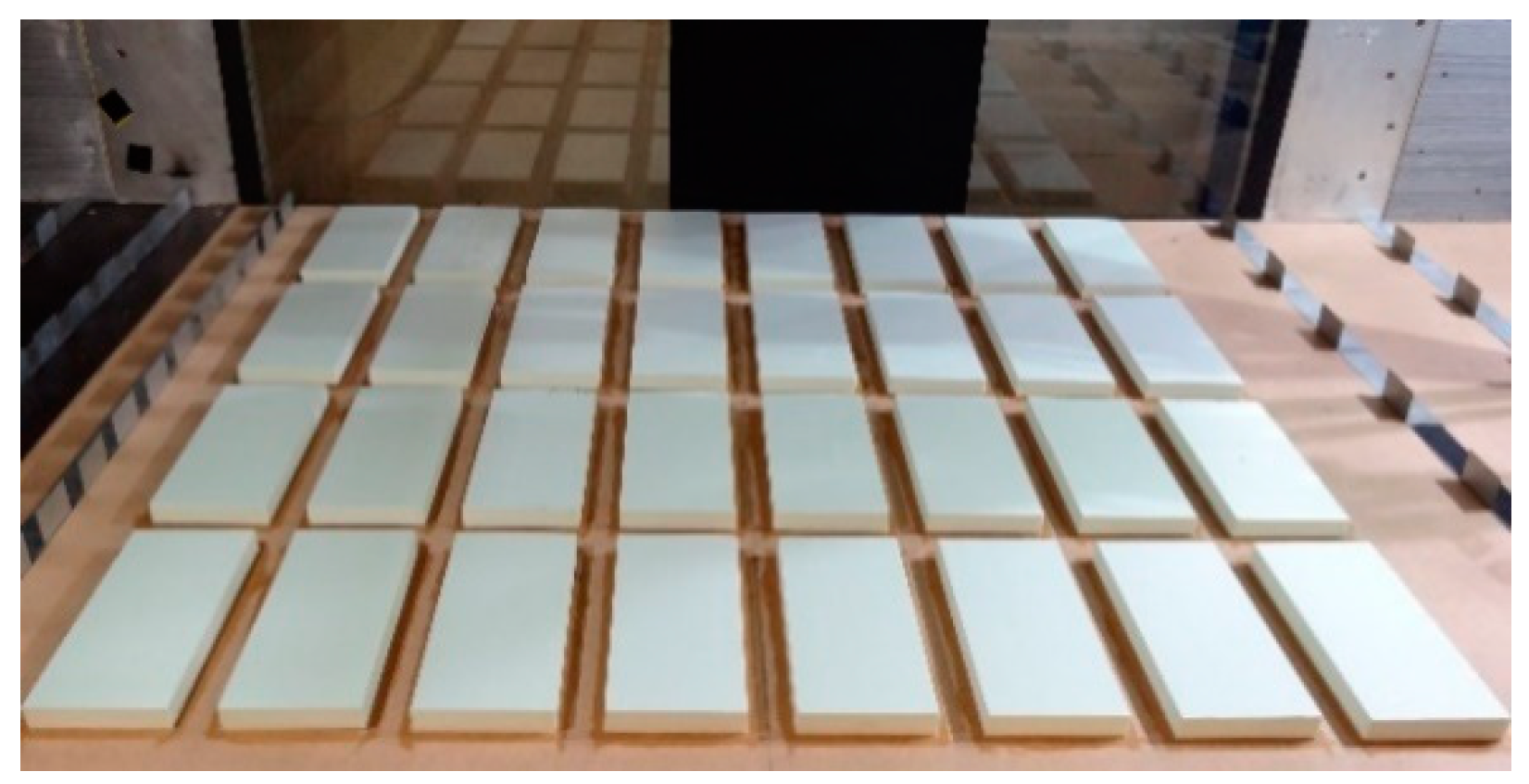
The experiments were conducted in an open-circuit low-speed wind tunnel, which is in the Laboratory of Environmental Aerodynamics of the Institute of Thermomechanics, in 2020. In the wind tunnel, an atmospheric boundary layer at a 1:400 scale with a neutral stratification similar to the one found in cities was modeled utilizing spires and roughness elements in the development section. The characteristics of the modeled boundary layer correspond to the Verein Deutcher Ingenier (VDI) requirements for these environments [29]—Table 1. The same boundary layer was utilized in [12,14,30,31,32]. The vertical profiles of the mean velocity and the intensity of turbulence of the velocity component along the main wind direction at the inlet section can be found in [14]. Into the wind tunnel test section, a model at the scale of 1:400 was placed. The model consisted of rectangular buildings (150 × 300 × 30 mm) with flat roofs positioned equidistantly from each other (50 mm, Figure 1). In contrast with [12,14,30,31,32], the model height is lower; the model houses do not have pitched roofs and no courtyards are present.
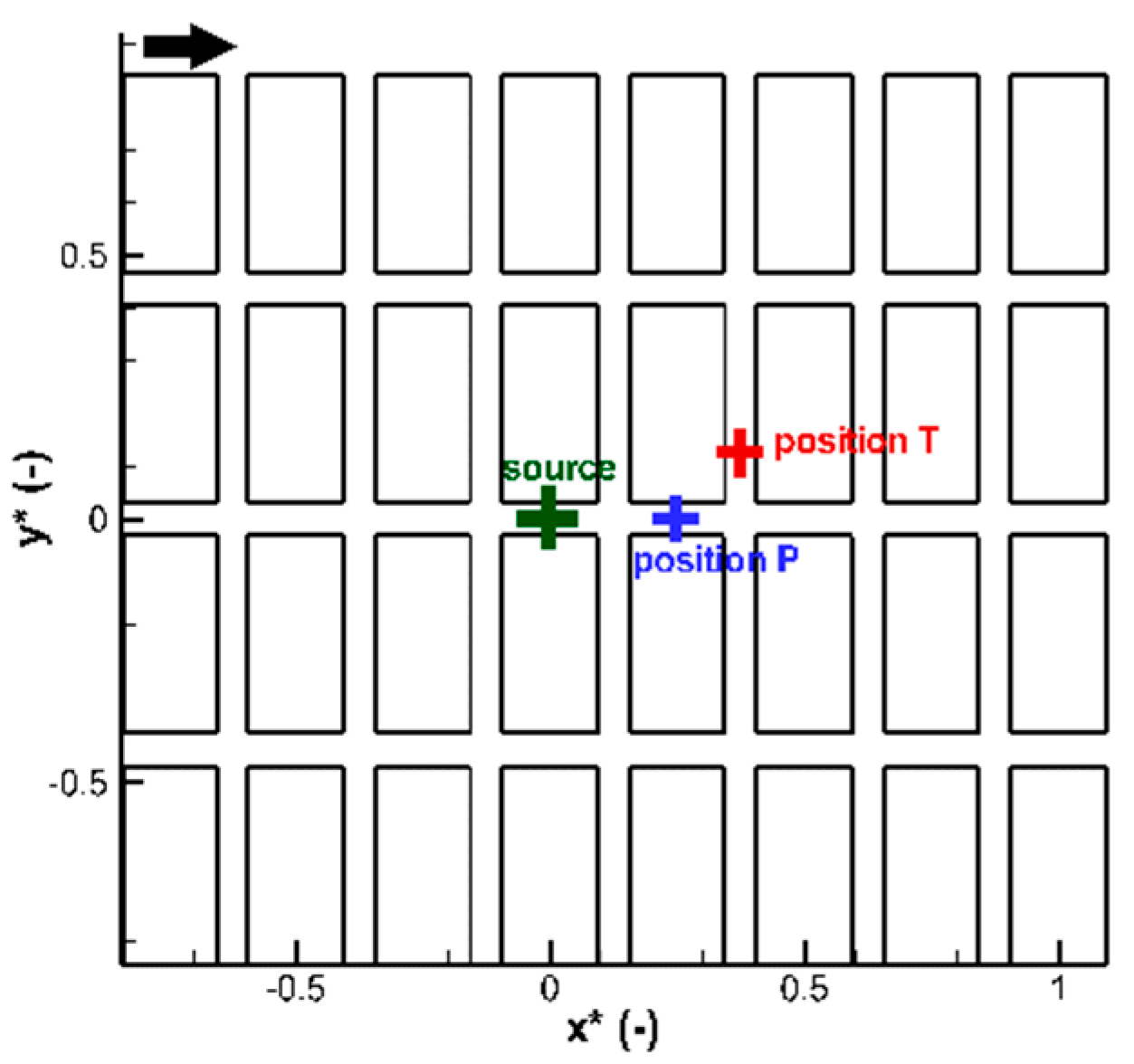
The finite-duration gas releases were created with usage of an electromagnetic valve. A ground level point gas source with a circular orifice with a 4 mm radius was positioned into the middle of a street parallel with the main flow direction (Figure 2). Pure ethane was utilized as a tracer gas. The constant flow rate of 5.6 mL/s was set by the Cole-Parmer Flowmeter. The duration of the short-term releases varied between 0.5 and 9 s. The release duration of the continuous releases was 180 s. The dispersion of gas after the release was recorded at two exposed positions by the fast flame ionization detector HFR400 of Cambustion, manufactured in England [33]. The response time of the detector was found to be better than 6 ms by a flick test. The details of the test can be found in [14]. The data were sampled at 1000 Hz and smoothed to 6 ms averages. The experiments were repeated for each detection location and release duration 400–600 times to acquire statistically representative datasets. In total, approximately 20,000 experiment repetitions were conducted. The first sampling position was situated on a street parallel with the main flow direction (position P). The second sampling position was set to a street transverse to the main flow direction (position T). The height of the measurement was chosen at the pedestrian level (z = 4 mm) since this level is the most important to assess the emergency risk.
2.2. Data Analysis
The concentration time series were nondimensionalized utilizing the following relations [29]:
- dimensionless coordinates;
- dimensionless time;
- dimensionless concentration utilizing plume scaling;
- dimensionless concentration utilizing puff scaling.
In the above relations, , (m) stand for the horizontal coordinates, (m/s) stands for the reference speed (which corresponds to the wind speed at the middle height of the wind tunnel and had the value between 1.8 and 6.7 m/s to be able to get the desired dimensionless release duration), (m) the characteristic height (the height of the modelled boundary layer 0.8 m), (s) is time, (kg∙s−1) is the source intensity, (kg) is the total amount of gas released, and (kg∙m−3) is the concentration. Appropriate experimental conditions were determined by conducting tests of independence of dimensionless concentrations (utilizing plume scaling) on Reynolds number as well as the source intensity. All the experiments were performed under these conditions.
In this paper, the following finite-duration release characteristics were utilized:
- arrival time (AT)
The arrival time for the analysis of mean concentration time series is defined as the time when the triple of the 99th percentile of the background concentrations is exceeded for the first time after the gas release;
- departure time (DT)
The departure time for the analysis of mean concentration time series is defined as the time when the triple of the 99th percentile of the background concentrations is exceeded for the last time after the gas release;
- maximum concentration
The maximum concentration is the highest concentration registered during the time when the cloud was at the sampling location (time interval AT–DT);
- peak time
The peak time is the time when the maximum concentration was detected.
3. Results and Discussion
3.1. Individual vs. Mean Finite-Duration Gas Releases
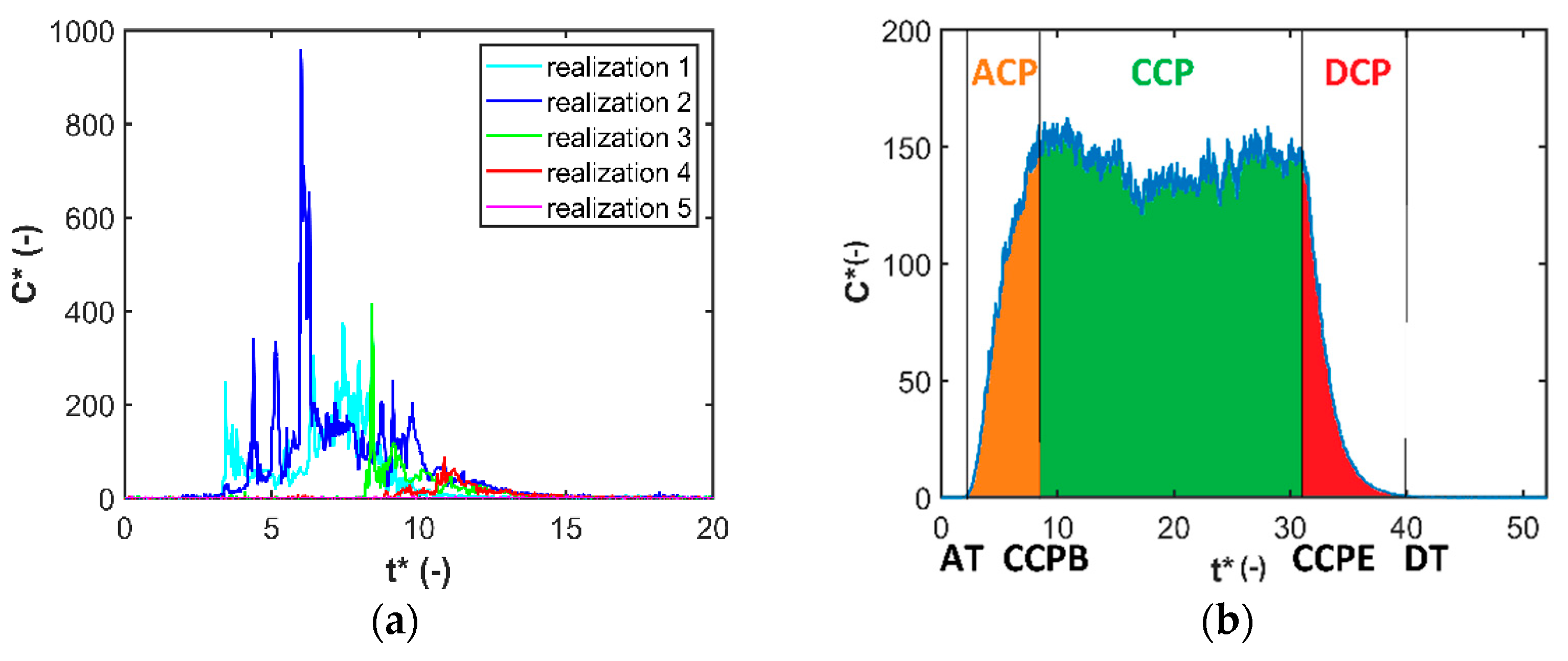
When the toxic gas cloud is released, it is being dispersed by the ambient air. By placing a detector at a location exposed by the release, one can see a cloud front, in which gas is usually extensively diluted with ambient clean air (arrival cloud phase—ACP). The reason for the dilution may be the smaller eddies (compared to the cloud size) positioned between the cloud’s leading edge and the ambient clean air. Then, a central cloud phase (CCP), in which the densest cloud part is present, reaches the aforementioned location. When the cloud already leaves the observed position (departure cloud phase—DCP), the cloud trailing edge is diluted again, and gas concentration decreases until the cloud is definitively out of the detector position. Unfortunately, these cloud phases are hard to recognize in the concentration time series looking at an experiment realization of the release due to the turbulent wind (Figure 3a). One can see to what extent the concentration time evolution observed at a fixed position can differ. This difference can be seen for various signal characteristics—e.g., the arrival time of the cloud (for the realization 1 AT ≈ 3, for the realization 4 AT ≈ 9), maximum concentration (for the realization 2 max ≈ 950, for the realization 4 max ≈ 50), the time interval when the cloud was present at the detection position (for the realization 2 Δcloud presence ≈ 15, for the realization 4 Δcloud presence ≈ 5). On top of this, the cloud does not even have to come to the detection position (see realization 5). However, by conducting a large number of release realizations under the same mean ambient and release conditions, a mean cloud behavior can be calculated. The individual cloud phases are much easier to be recognized in this mean concentration signal (Figure 3b).
The approach of division of the finite-duration releases into the three phases have also been used in the mathematical modeling. For instance, the Atmospheric Dispersion Modelling System (ADMS) model [34] defines front end, rear end and plateau regions, which are analogous to our ACP, DCP, and CCP for the finite-duration releases. For the end parts, the ADMS model computes the concentrations using a Gaussian distribution multiplied by an exponential function, while it models the concentrations of the plateau region using the plume model approach.
3.2. Identification of the Individual Cloud Phases
The concentration begins to increase above the background level at the cloud arrival (AT). At a point in time, the signal looks frayed (i.e., higher concentration values are followed by a little lower ones and relatively no long steep increase or decrease can be seen in comparison with the very beginning of the cloud arrival/departure). This time point seems to be the one at which the arrival cloud phase (ACP), starting with the first gas arrival (AT), switches to the central cloud phase (CCP).
The switching time can be found connecting two points of the concentration time series with a segment line and looking at its slope. The first fixed point of the line segment is a point positioned in time before the arrival time whose exact position must be further particularized (see the paragraph below). The second point is gradually chosen as a point of the time series from the arrival time to the departure time and, for each segment line, its slope is calculated. The line slope generally increases forming a peak and then starts to decline. The maximum of these slopes is the candidate for the beginning of CCP (CCPB) (Figure 4a).
The exact position of the line segment fixed point must be sought. It is a point before the arrival time but the shift before the arrival time is different for different time series. One has to look at the value of the candidate for CCPB while moving with the point against the direction of the time beginning with the arrival time. CCPB can change at first but then it stays constant and this is the correct value of CCPB (Figure 4b). The reason for the necessity of this approach is that sometimes the slope of the line segment can be higher for a point still in the region of the relatively steep increase in the concentrations if the fixed point is too close to the arrival time. The end of CCP (CCPE) can be found by a similar approach. The only difference is that the moving left point of the segment line is a point in time in the region bounded by the departure time and the arrival time. The fixed point is a point in time after the departure time.
Concentration time series of individual cloud realizations are then split into individual cloud phases utilizing the found limits. Then, the phases of each realization can be analyzed (e.g., mean or maximum can be sought). Ensemble characteristics (e.g., means) can be then calculated using the characteristics values of individual realizations. In the paper, we used the ensemble means of cloud phase means (of individual realizations), the ensemble means of entire cloud means (calculated from the time interval AT–DT for each realization), and the ensemble means of maximum concentrations (of individual realizations).
3.3. Length of Cloud Phases
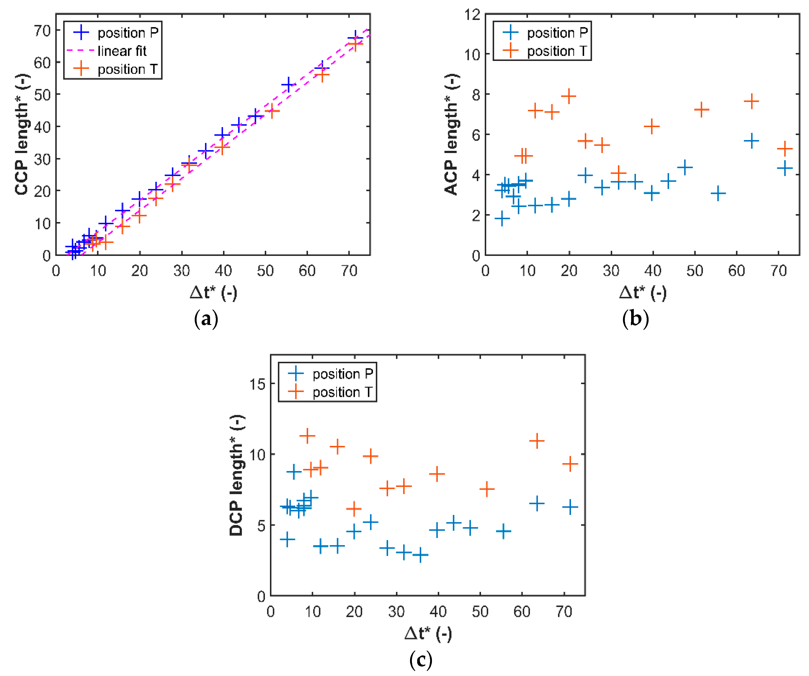
The lengths of individual cloud phases are plotted in Figure 5. The CCP length, ascertained from the ensemble mean concentration time series, increased linearly with the increase in the release duration Δt*. Moreover, the release duration from which CCP should be detectable can be found by utilizing the fitted line. The fitting could be negatively influenced by the values for the release durations lower than six for which the CCP length is zero or a small positive value for position T. Hence, these results were excluded from the analysis. The linear regression revealed that CCP should be recognizable in the mean concentration time series from the release duration Δt* = 2.6 ± 0.6 for position P and Δt* = 6 ± 2 for position T. These values might be the candidates for the switching duration between the plume and puff dispersion types. It can be seen that these values depend on the detection position, which contradicts the hypothesis that the value 1 h of the Van der Hoven energy spectrum gap might be the searched value [26]. Compared to the Pasquill and Smith hypothesis [27], which determines the switching release duration as the cloud travel time from the source to the sampling position, the found values are, especially for position P, lower. The phase is shorter at position T than at position P for the same release duration since the cloud is more diffused in the position further from the source and the dense cloud part is therefore smaller.
Contrary to CCP, the lengths of ACP and CCP are practically independent of the release duration Δt*. The mean length of ACP has a tendency to be shorter than DCP. The reason for this is that the cloud is more dispersed in the later times from when the release started. Both edge phases tended to be longer at position T as the cloud is more dispersed at this position and the diluted phases are therefore larger.
3.4. CCP Behaviour
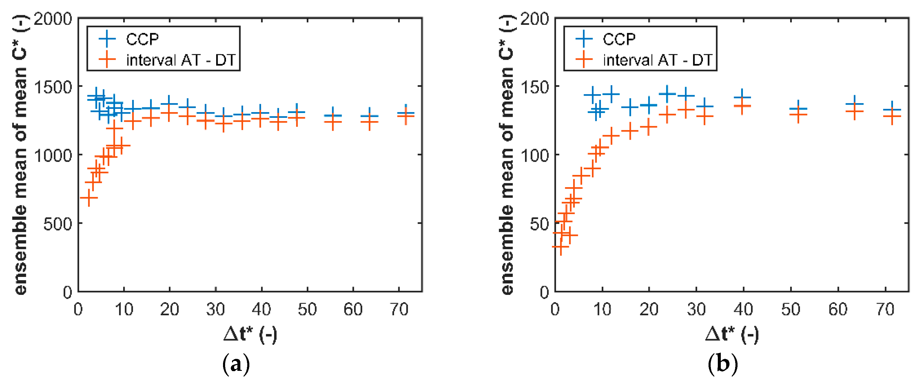
Out of all of the phases, the central cloud phase (CCP) should be the phase most similar to the continuous release. Figure 6 shows the comparison of the ensemble mean of CCP mean concentrations for various release durations. The values on the graph oscillate about the value of the mean concentration for the continuous release (1300 ± 20 for position P, 140 ± 10 for position T) for all release durations. However, higher variations can be found for values lower than 10. The ADMS model [34] calculates the plateau region of the finite-duration releases by the same approach as the plume model. Hence, our finding that the ensemble means of CCP mean concentration agrees with the value of the mean concentration for the continuous release backs up the ADMS model approach of the plateau region modeling.
The change in the variability of concentrations in the CCP phase was also explored. The results showed that the variability is independent for all release durations for position P. However, this was not true for position T for which the constancy was not reached until the release duration Δt* was approximately 30. We tried to explore whether this characteristic was a matter of shortness of the time intervals used for the calculations. Hence, we split the time series of the continuous release into intervals of the same length as those for the finite-duration releases. The variations for these were calculated and the mean value was compared to the variation calculated from the entire time series of the continuous release. The values calculated from the short intervals were a few times smaller. These multiples were then utilized to correct the variability values of the finite-duration releases. Then, the variability was found to be independent of the release duration.
We also tried a different approach to assess the correctness of the method described above. We took the CCP intervals of all realizations and created a long concentration time series from them. From this series, the variability was calculated. This approach was made for all release durations. The calculated values were found to be similar to the ones with usage of the multiples. We also verified the results of ensemble means of means CCP utilizing a long time series approach for calculation of the means. The differences between the results found by both methods were negligible.
3.5. Cloud Edges
Figure 6 can be used for the evaluation of the influence of the cloud edges—ACP and DCP—on the entire cloud (time interval AT–DT). The graph shows that the mean values calculated from the time interval AT–DT increase until a state of saturation was reached. A huge difference between the values of CCP and the entire cloud is seen for small release durations. Hence, the extraction of CCP from the entire puff is significant for the resultant value for these release durations. However, moving towards high release durations, this difference becomes very small, even though the values are still very slowly getting closer to each other.
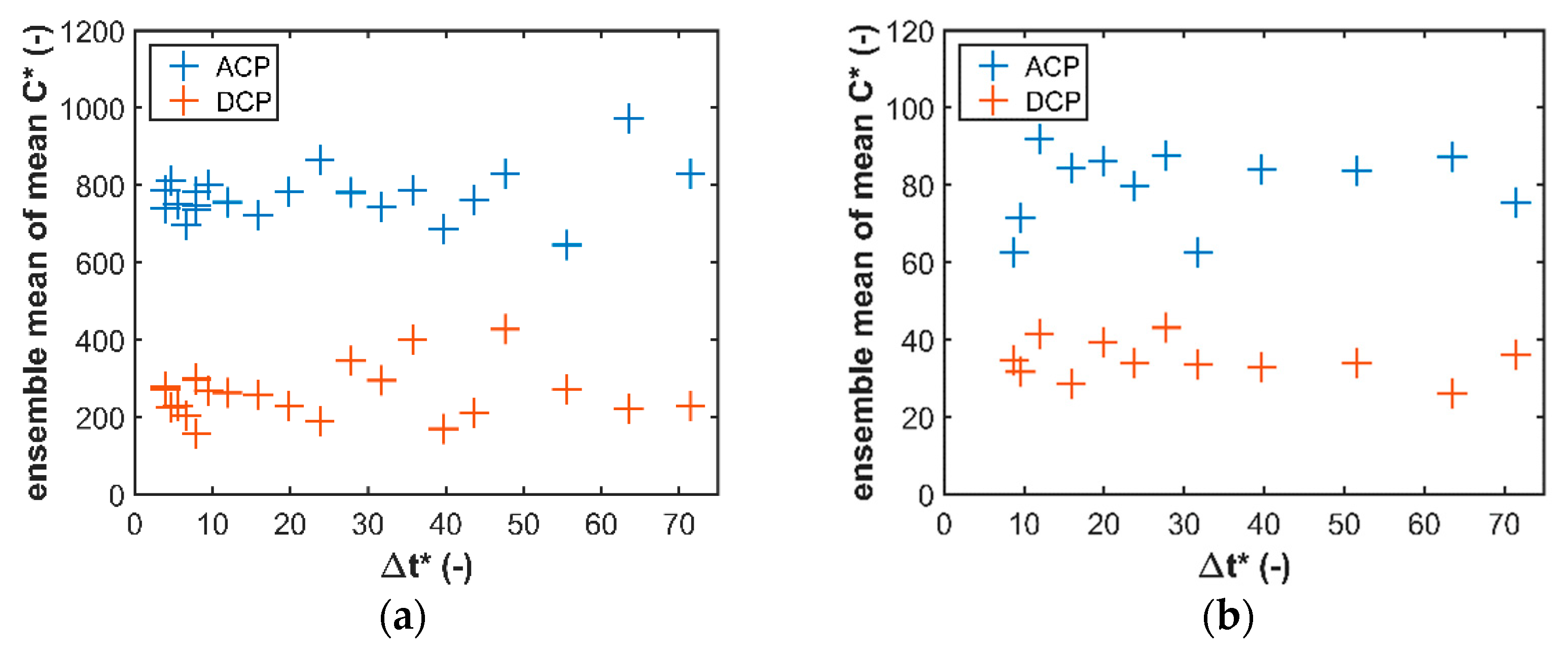
The ensemble mean of the mean ACP concentrations is independent of the release duration (Figure 7). Its value is 800 ± 200 for position P and 80 ± 20 for position T. The ensemble mean of the mean DCP concentrations is also independent of the release duration with its mean value 300 ± 100 for position P and 36 ± 7 for position T. These findings of the cloud edges’ independence from the release duration are in agreement with the modeling approach of the ADMS model [34]. The values of ACP generally tend to be higher than the values of DCP. The reason for this is that the DCP length tends to be longer than the ACP length. One can see a typical tail observable as a steep decrease in concentration slowing down into a curve shaped like an arch (Figure 3b). The concentrations in this region are still not that of the background level but are relatively low.
3.6. Ensemble Mean of Maximum Concentration
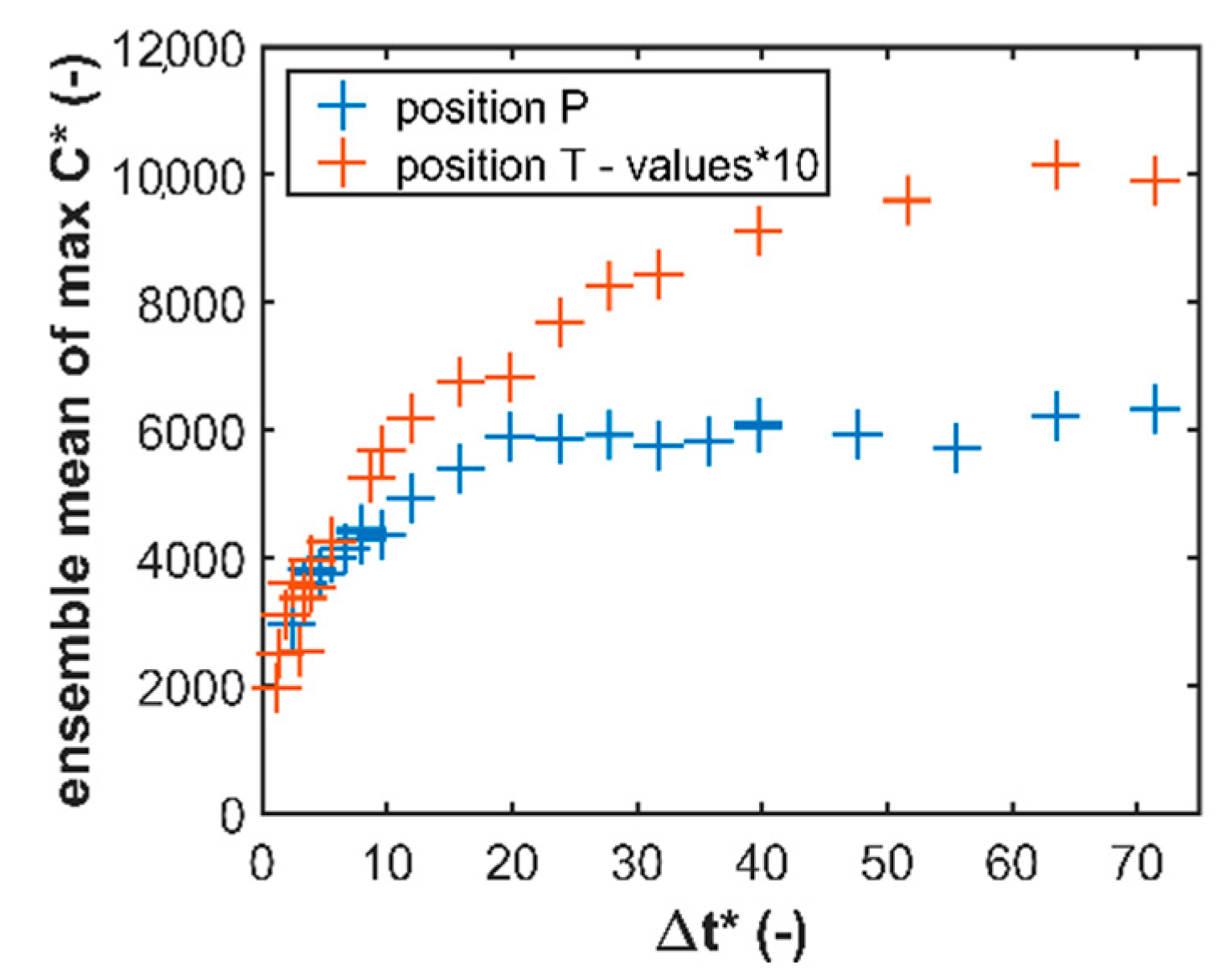
Figure 8 shows the change in the ensemble mean of maximum concentration with an increase in the release duration utilizing the plume scaling (Equation (3)). The data for both sampling positions demonstrate the same behavior. With the increase in the release duration, the values increase at first but from a specific duration, the values become constant, which confirms the statement of Robins and Fackrell [28]. Moreover, the increase in the ensemble mean of maximum concentration with an increase in the release duration for small release durations was also observed in [30]. The described behavior can be explained as follows—the cloud was being diluted at the front of the cloud until the dense center of the cloud came to the detection location. When the cloud left the sampling position, the concentration started to decrease again. For the shortest releases, the phase of increasing the concentration is stopped by the beginning of the cloud departure at the detection location. By prolonging the release duration, the phase of concentration growth becomes longer, hence higher maximum concentrations can be observed. With further prolonging, one can see a phase, in which concentrations are in a relatively stable phase being seen as a plateau region in graphs of mean clouds. At first, it holds that the longer this time interval is, the higher the probability that a huge concentration will be registered in a realization. However, when the plateau region is sufficiently long enough, the value of the mean maximum concentration stays constant. This behavior might indicate that mixing of gas within the cloud is caused by the eddies smaller than that of the cloud.
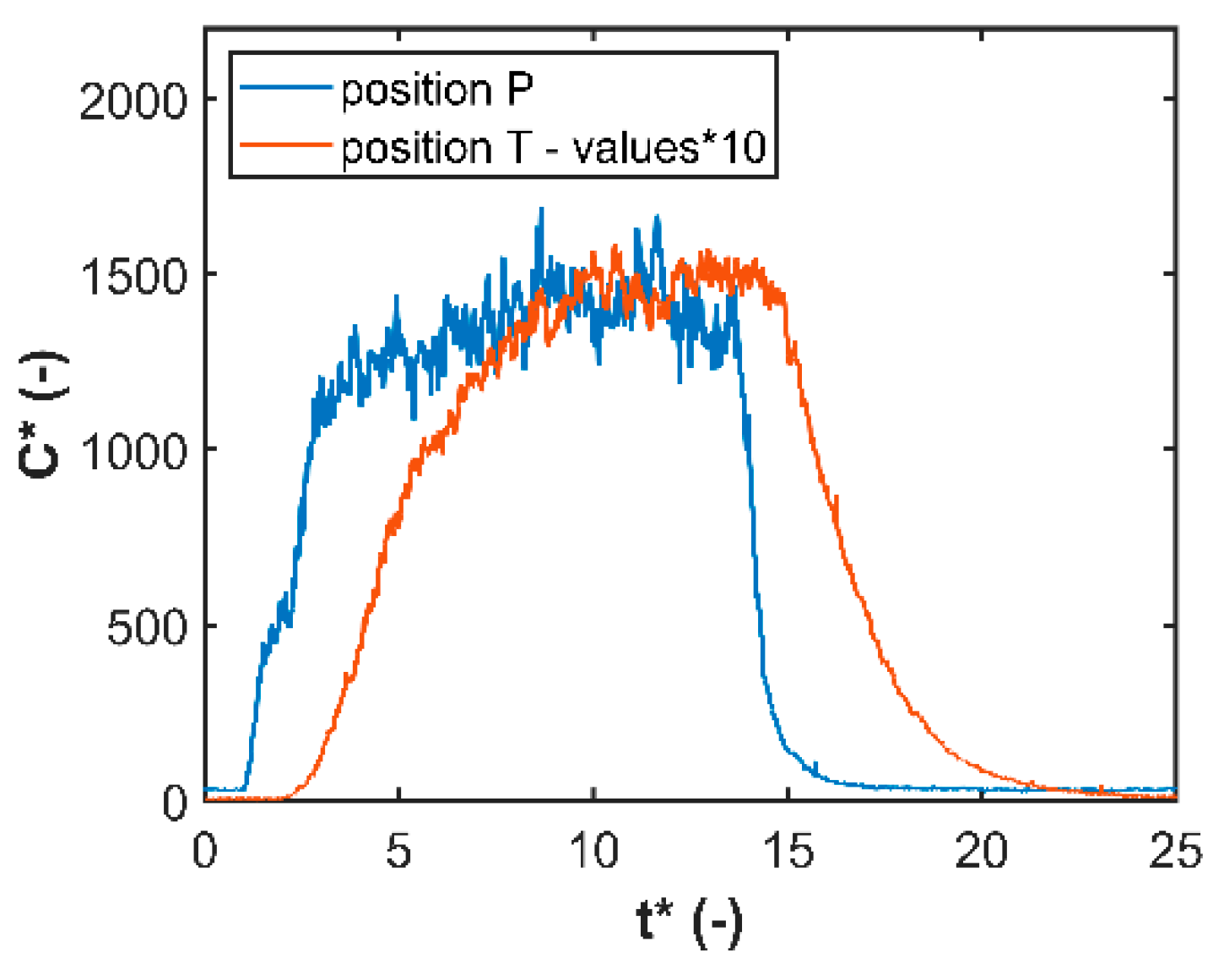
Robins and Fackrell [28] report that the plateau region becomes clear when constancy of the ensemble mean of maximum concentration is reached. For our measurements, however, the plateau region was observed, especially at position T, much earlier (Figure 9). One can see that the constancy of the values is reached approximately for the release duration Δ = 20 for the position P (60 for the position T) in Figure 8 but Figure 9 illustrates that even the release of the duration Δ = 12 has a visible plateau region for both positions. The reason for the different behavior with the compared study could be the different conditions for gas dispersion in the surrounding environment—the presence of obstacles in contrast with the compared study. The buildings cause the cloud to distort and gas to be redistributed, which might result in the possibility of seeing the plateau region for the shorter release durations.
Figure 10 shows the dependence of the mean maximum concentration on the release duration utilizing the puff scaling (Equation (4)). Robins and Fackrell [28] state that measurements with Δ < 4 of their graph represent a plateau region in which the cloud appears as if it had puff behavior. In contrast with these, no region in which constant values are present was observed in our measurements. The reason for this might be the different conditions for gas dispersion in the surrounding environment as described in detail in the paragraph above. All in all, our data indicate that the constant region does not always need to be present and cannot be generally used to distinguish between the two cloud regimes—i.e., the puff and the plume.
3.7. General Set of Criteria for Cloud Regimes
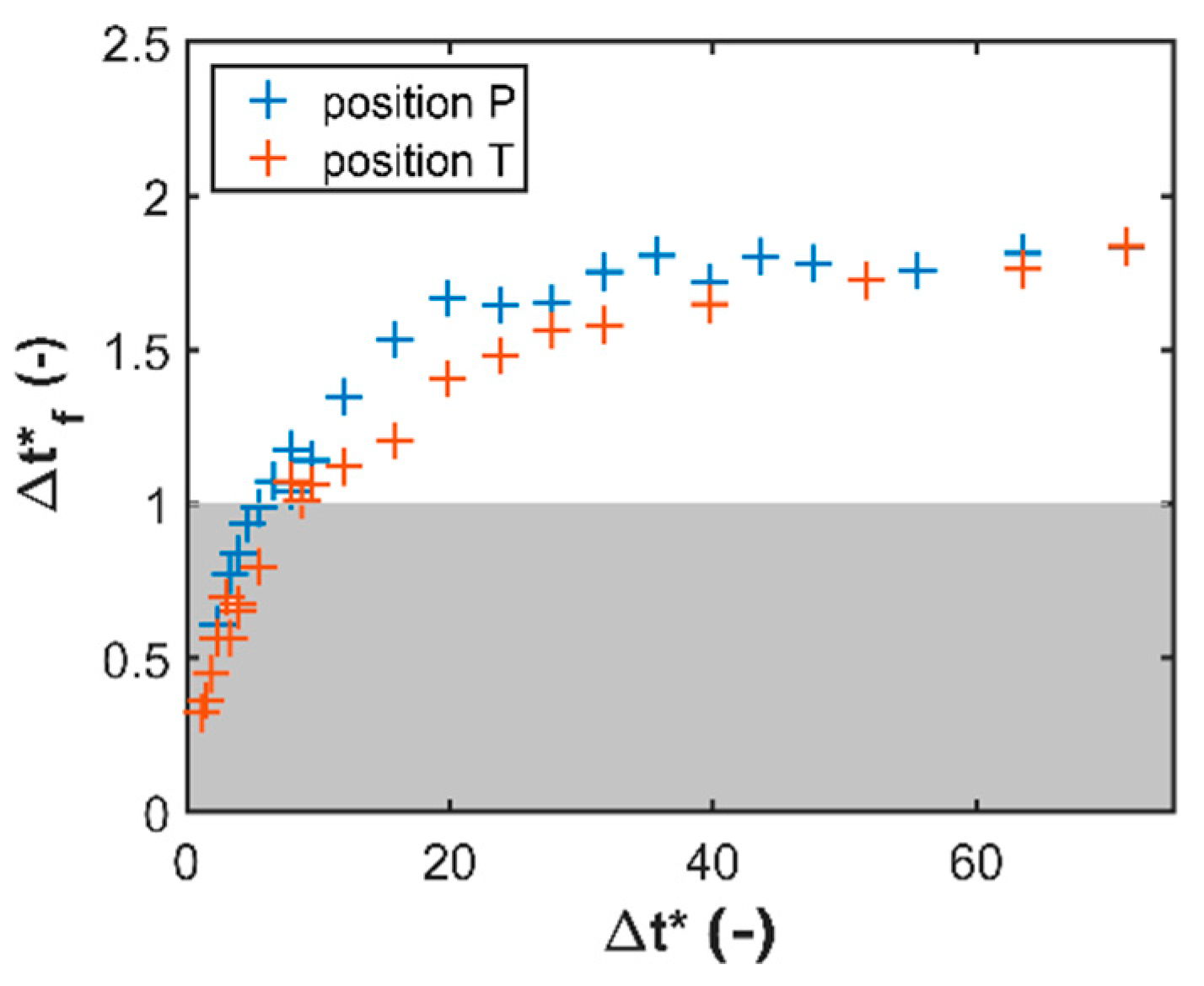
Robins and Fackrell [28] suggest that a general set of cloud regime criteria is enabled utilizing a time scaling Δf = Δ/travel time. For the values equal to or higher than 1, plume behavior should be observed. Robins and Fackrell defined the travel time as the time at which maximum concentration was detected for Δ < 10. They used a different definition for higher release durations for the travel time (the mean of arrival and departure time which were calculated as the time at which a half of the plateau concentration was reached). In contrast, we utilized the time at which maximum concentration was detected as the definition of the travel time for all release durations. The value Δf = 1 was approximately reached for Δ = 6 for position P and 8 for position T in our measurements. This value is not far from Δ = 10 from which a different definition should be utilized. Hence, any change in behavior on the graph could be caused by the change in the definition of the travel time and not the change in the plume behavior. Therefore, we decided to use the same definition of travel time for the all studied cases.
No change in behavior of the dependence of Δf on Δ was seen for our datasets (Figure 11). In other words, our measurements did not confirm Pasquill and Smith’s [12] suggestions that different behaviors should be seen for the clouds travelling to the sampling position earlier than the gas release ended in a comparison with the clouds that travelled at the later time.
4. Conclusions
The paper focused on gas releases of finite-duration dispersed in a simplified urban area. It reveals that however wildly the concentration signal can change at a detection position from experiment realization to realization, the mean signals calculated from ensembles enable the extraction of three cloud phases. These phases are: the arrival cloud phase (ACP), the central cloud phase (CCP) and the departure cloud phase (DCP).
The method for the extraction of the phases is based on the plotting of two segment lines in the graph of mean concentration time series. The first point of the segment lines was positioned before (after) the cloud arrival (departure). The second point of both lines was selected from the interval between the arrival and departure time of the cloud. It is chosen so the slope of the segment line has the highest possible value. These second points of the segment lines bound CCP. ACP, starting with arrival time (AT), was positioned just before CCP. In contrast, DCP, ending with departure time (DT), was placed just after CCP.
CCP is the cloud phase most similar to the continuous gas release. The ensemble mean of mean CCP concentration oscillate about the mean value of concentration valid for continuous release. However, one can spot higher variations for the release durations lower than 10. The length of CCP increases proportionally with the release duration. Using this finding, one can find the minimum release duration from which CCP can be observed.
Cloud edges—ACP and DCP—are the phases at which the cloud is diluted by the ambient clean air. Their influence is dominant while calculating the mean concentrations of the entire cloud (interval AT–DT) for short release durations (approximately lower than 30). The mean ACP concentration and DCP concentration are independent of the release duration. The values of mean ACP concentration tend to be higher than the values of mean DCP concentration as DCP has a relatively long tail with low concentrations.
Investigations of mean maximum concentrations and ratio of release duration to cloud travel time for different release durations did not give any clues to help distinguish the puff and plume behaviors in contrast to Robins and Fackrell’s [28] research. The reason for this is probably the different environment to which the gas is being dispersed.
All in all, this paper revealed how the mean concentration time series obtained by wind tunnel modeling can be split into three phases from a specific release duration dependent on the position towards the source of contaminant. The middle phase, containing the dense part of the cloud, evinces characteristics similar to the continuous release. Moreover, the paper showed an approach to find the smallest release duration from which the middle phase can be seen for the given detection position. More research is essential to discover how the release duration when CCP starts to form changes with respect to the detection position.
Author Contributions
H.C. conducted measurements in the wind tunnel. She also analyzed the obtained data and wrote the paper. Z.K. conducted the measurements in the wind tunnel and revised the paper. R.K. conducted measurements and made the revisions of the paper. Z.J. made the revisions of the paper. All authors have read and agreed to the published version of the manuscript.
Funding
This research was funded by the Technology Agency of the Czech Republic, grant TJ04000365 of the program Zéta 4 and by the Institute of Thermomechanics, Academy of Sciences, Czech Republic—RVO: 6138998.
Data Availability Statement
Data available on request.
Conflicts of Interest
The authors declare no conflict of interest.
References
- Baumann-Stanzer, K.; Andronopoulos, S.; Armand, P.; Berbekar, E.; Efthimiou, G.; Fuka, V.; Gariazzo, C.; Gasparac, G.; Harms, F.; Hellsten, A.; et al. COST ES1006 Model Evaluation Case Studies: Approach and Results, 1st ed.; COST Office: Hamburg, Germany, 2015; p. 114. [Google Scholar]
- Balczo, M.; Di Sabatino, S.; Franke, J.; Grebec, M.; Karpinnen, A.; Meijer, E.; Moussafir, J.; Reif, B.P.; Tinsrelli, G.; Trijssenaar-Buhre, I. COST ES1006-Background and Justification Document, 1st ed.; COST Office: Hamburg, Germany, 2012; p. 88. [Google Scholar]
- Di Gilio, A.; Palmisani, J.; Trizio, L.; Saracino, G.; Giua, R.; de Gennaro, G. Total p-PAH Levels Nearby a Complex Industrial Area: A Tailored Monitoring Experiment to Assess the Impact of Emission Sources. Atmosphere 2020, 11, 469. [Google Scholar] [CrossRef]
- Smit, R.; Kingston, P. Measuring On-Road Vehicle Emissions with Multiple Instruments Including Remote Sensing. Atmosphere 2019, 10, 516. [Google Scholar] [CrossRef] [Green Version]
- Filippi, J.B.; Bosseur, F.; Mari, C.; Lac, C. Simulation of a Large Wildfire in a Coupled Fire-Atmosphere Model. Atmosphere 2018, 9, 218. [Google Scholar] [CrossRef] [Green Version]
- Prichard, S.; Larkin, N.S.; Ottmar, R.; French, N.H.; Baker, K.; Brown, T.; Clements, C.; Dickinson, M.; Hudak, A.; Kochanski, A.; et al. The Fire and Smoke Model Evaluation Experiment—A Plan for Integrated, Large Fire–Atmosphere Field Campaigns. Atmosphere 2019, 10, 66. [Google Scholar] [CrossRef] [Green Version]
- Netterville, D.D.J. Concentration Fluctuations in Plumes; Syncrude; Canada Ltd.: Edmonton, AB, Canada, 1979; p. 228. [Google Scholar]
- Fackrell, J.E. A flame ionisation detector for measuring fluctuating concentration. J. Phys. E Sci. Instrum. 1980, 13, 888–893. [Google Scholar] [CrossRef]
- Finn, D.; Clawson, K.L.; Carter, R.G.; Rich, J.D.; Biltoft, C.; Leach, M. Analysis of urban atmosphere plume concentration fluctuations. Bound. Layer Meteorol. 2010, 136, 431–456. [Google Scholar] [CrossRef] [Green Version]
- Yea, E.; Kosteniuk, P.R.; Chandler, G.M.; Biltoft, C.A.; Bowers, J.F. Statistical characteristics of concentration fluctuations in dispersing plumes in the atmospheric surface layer. Bound. Layer Meteorol. 1993, 65, 69–109. [Google Scholar] [CrossRef]
- Harms, F.; Leitl, B.; Hertwig, D.; Schatzmann, M. Atmospheric variability and its implications in validating urban flow and dispersion models. In Proceedings of the Sixth International Symposium on Computational Wind Engineering, Hamburg, Germany, 8–12 June 2014. [Google Scholar]
- Chaloupecká, H.; Jakubcová, M.; Jaňour, Z.; Jurčáková, K.; Kellnerová, R. Equations of a new puff model for idealized urban canopy. Process Safety Environ. Prot. 2019, 126, 382–392. [Google Scholar] [CrossRef]
- Hanna, S. Puff or Plume? In Proceedings of the 18th Joint Conference on the Applications of Air Pollution Meteorology with the A&WMA, Atlanta, GA, USA, 2–6 February 2014.
- Chaloupecká, H.; Jaňour, Z.; Mikšovský, J.; Jurčáková, K.; Kellnerová, R. Evaluation of a new method for puff arrival time as assessed through wind tunnel modelling. Process Saf. Env. Ment. Prot. 2017, 111, 194–210. [Google Scholar] [CrossRef]
- Zimmerman, P.C.; Chatwin, W.B. Fluctuations in dense gas concentrations measured in a wind tunnel. Bound. Layer Meteorol. 1995, 75, 321–352. [Google Scholar] [CrossRef]
- Doran, J.C.; Alwine, K.J.; Flaherty, J.E.; Clawson, K.L.; Carter, R.G. Characteristics of puff dispersion in an urban environment. Atmos. Environ. 2007, 41, 3440–3452. [Google Scholar] [CrossRef]
- Zhou, Y.; Hanna, S.R. Along-wind dispersion of puffs released in a built-up urban area. Bound. Layer Meteorol. 2007, 125, 469–486. [Google Scholar] [CrossRef]
- Ficher, R.; Schatzmann, M.; Leitl, B. How often is sufficient? A program of the statistical analysis of puff dispersion in urban environments. In Proceedings of the PHYSMOD, Orleans, France, 29–31 August 2007. [Google Scholar]
- Gifford, F.A. An outline of theories of diffusion in the lower layers of the atmosphere. Meteorol. At. Energy 1968, 3, 66–116. [Google Scholar]
- Hanna, S.; Briggs, G.; Hosker, R. Handbook on Atmospheric Diffusion; Technical Information Center U. S. Department of Energy: Springfield, IL, USA, 1928; p. 102.
- Taylor, G.I. Diffusion by continuous movements. Proc. Lond. Math. Soc. 1921, 20, 196. [Google Scholar] [CrossRef]
- Batchelor, G.K. Application of the similarity theory of turbulence to atmospheric diffusion. QJR. Meteorol. Soc. 1950, 76, 133–146. [Google Scholar] [CrossRef]
- Hanna, S.; Chang, J. Dependence of maximum concentration from chemical accidents on release duration. Atmos. Environ. 2017, 148, 1–7. [Google Scholar] [CrossRef] [Green Version]
- Hanna, S.; Britter, R.; Argenta, E.; Chang, J. The Jack Rabbit chlorine release experiments: Dense gas removal from a depression by crosswinds. J. Hazard. Mater. 2012, 213, 406–412. [Google Scholar] [CrossRef]
- Hanna, S.; Chang, J.; Huq, P. Observed chlorine concentrations during Jack Rabbit I and Lyme Bay field experiments. Atmos. Environ. 2016, 125, 252–256. [Google Scholar] [CrossRef]
- Van der Hoven, I. Power spectrum of horizontal wind speed in the frequency range from 0.0007 to 900 cycles per hour. J. Meteorol. 1954, 14, 160–164. [Google Scholar] [CrossRef] [Green Version]
- Pasquill, F.; Smith, F.B. Atmospheric Diffusion, 3rd ed.; John Wiley & Sons: Chichester, UK, 1984. [Google Scholar]
- Robins, A.G.; Fackrell, J.E. An experimental study of the dispersion of short duration emissions in a turbulent boundary layer. WIT Trans. Ecol. Environ. 1998, 28. [Google Scholar] [CrossRef]
- Verein Deutcher Ingenier. Environmental Meteorology, Physical Modelling of Flow and Dispersion Processes in the Atmospheric Boundary Layer, Application of Wind Tunnels, 1st ed.; Verein Deutcher Ingenier: Dusserdorf, Germany, 2000. [Google Scholar]
- Chaloupecká, H.; Jaňour, Z.; Jurčáková, K.; Kukačka, L.; Nosek, Š. Sudden releases of gases. Eur. Phys. J. 2014, 67. [Google Scholar] [CrossRef] [Green Version]
- Chaloupecká, H.; Jaňour, Z.; Kellnerová, R.; Jurčáková, K. Influence of Flow on Puff Characteristics. In WIT Transactions on Engineering Sciences, 1st ed.; Villacampa, Y., Carlomagno, G.M., Ivorra, S., Brebbiaeds, C.A., Eds.; Witpress: Winchester, UK, 2017; pp. 37–48. [Google Scholar]
- Chaloupecká, H.; Jaňour, Z.; Jurčáková, K.; Kellnerová, R. Sensitivity of puff characteristics to maximum-concentration-based definition of departure time. J. Loss Prev. Process Ind. 2018, 56, 242–253. [Google Scholar] [CrossRef]
- HFR400 Atmospheric Fast FID, User Guide, 1st ed.; Cambustion Ltd.: Cambridge, UK, 2017.
- CERC. Puff/Plume Spread and Mean Concentration Module Specifications, 1st ed.; CERC: Cambridge, UK, 2020. [Google Scholar]
Figure 1.
The wind tunnel test section with the model.

Figure 2.
Layout of the model with the sampling positions (position P, T) and the gas source position represented by the crosses. The arrow direction is the direction of the main flow.
Figure 2.
Layout of the model with the sampling positions (position P, T) and the gas source position represented by the crosses. The arrow direction is the direction of the main flow.

Figure 3.
Finite-duration gas release concentration time series: (a) a few individual realizations; (b) mean behavior (the blue signal represents the concentration averaged over all realizations at individual times after the gas release; ACP stands for the arrival cloud phase, CCP the central cloud phase and DCP the departure cloud phase).

Figure 4.
Finding the beginning of CCP (CCPB): (a) slopes of segment lines; (b) finding the correct CCPB.
Figure 4.
Finding the beginning of CCP (CCPB): (a) slopes of segment lines; (b) finding the correct CCPB.

Figure 5.
The length of the cloud phases: (a) the central cloud phase (CCP); (b) the arrival cloud phase (ACP); (c) the departure cloud phase (DCP).
Figure 5.
The length of the cloud phases: (a) the central cloud phase (CCP); (b) the arrival cloud phase (ACP); (c) the departure cloud phase (DCP).

Figure 6.
Comparison of the ensemble mean of CCP mean concentrations and the mean concentrations calculated from entire clouds (time interval arrival time (AT)–departure time (DT)) for: (a) position P; (b) position T.
Figure 6.
Comparison of the ensemble mean of CCP mean concentrations and the mean concentrations calculated from entire clouds (time interval arrival time (AT)–departure time (DT)) for: (a) position P; (b) position T.

Figure 7.
Ensemble mean of mean ACP and DCP for: (a) position P; (b) position T.

Figure 8.
Ensemble mean of maximum concentration (note: the statement values*10 means that the values were multiplied by 10 to be able to show the results of both positions in one figure).
Figure 8.
Ensemble mean of maximum concentration (note: the statement values*10 means that the values were multiplied by 10 to be able to show the results of both positions in one figure).

Figure 9.
Mean concentration time series for the clouds with the release duration 12 for both explored positions (note: the statement values*10 means that the values were multiplied by 10 to be able to show the results of both positions in one figure).
Figure 9.
Mean concentration time series for the clouds with the release duration 12 for both explored positions (note: the statement values*10 means that the values were multiplied by 10 to be able to show the results of both positions in one figure).

Figure 10.
Dependence of the mean maximum concentration on the release duration utilizing puff scaling (note: the statement values*15 means that the values were multiplied by 15 to be able to show the results of both positions in one figure).
Figure 10.
Dependence of the mean maximum concentration on the release duration utilizing puff scaling (note: the statement values*15 means that the values were multiplied by 15 to be able to show the results of both positions in one figure).

Figure 11.
Dependence of Δf on Δ.


Table 1.
Boundary layer characteristics—modeled values and the recommended values by the Verein Deutcher Ingenier (VDI) documentation [29].
Table 1.
Boundary layer characteristics—modeled values and the recommended values by the Verein Deutcher Ingenier (VDI) documentation [29].
| Parameter | Value | VDI Value |
|---|---|---|
| Roughness length z0 (m) | 1.8 | 0.5–2.0 |
| Zero plane displacement d0 (m) | 3 | 2–15 |
| Power law exponent α (-) | 0.27 | 0.24–0.40 |
Publisher’s Note: MDPI stays neutral with regard to jurisdictional claims in published maps and institutional affiliations. |
© 2021 by the authors. Licensee MDPI, Basel, Switzerland. This article is an open access article distributed under the terms and conditions of the Creative Commons Attribution (CC BY) license (http://creativecommons.org/licenses/by/4.0/).
Share and Cite
MDPI and ACS Style
Chaloupecká, H.; Kluková, Z.; Kellnerová, R.; Jaňour, Z. Characteristics of Toxic Gas Leakages with Change in Duration. Atmosphere 2021, 12, 88. https://doi.org/10.3390/atmos12010088
AMA Style
Chaloupecká H, Kluková Z, Kellnerová R, Jaňour Z. Characteristics of Toxic Gas Leakages with Change in Duration. Atmosphere. 2021; 12(1):88. https://doi.org/10.3390/atmos12010088
Chicago/Turabian StyleChaloupecká, Hana, Zuzana Kluková, Radka Kellnerová, and Zbyněk Jaňour. 2021. "Characteristics of Toxic Gas Leakages with Change in Duration" Atmosphere 12, no. 1: 88. https://doi.org/10.3390/atmos12010088
Note that from the first issue of 2016, this journal uses article numbers instead of page numbers. See further details here.