Possible Increase of Vegetation Exposure to Spring Frost under Climate Change in Switzerland


1
Global Change Research Institute of the Czech Academy of Sciences, 60300 Brno, Czech Republic
2
Institute of Atmospheric Physics of the Czech Academy of Sciences, 14100 Prague, Czech Republic
3
Oeschger Centre for Climate Change Research and Institute of Geography, University of Bern, 3012 Bern, Switzerland
*
Author to whom correspondence should be addressed.
Atmosphere 2020, 11(4), 391; https://doi.org/10.3390/atmos11040391
Submission received: 27 February 2020
/
Revised: 31 March 2020
/
Accepted: 10 April 2020
/
Published: 15 April 2020
(This article belongs to the Special Issue Climate Events and Extreme Weather)
Abstract
:We assessed future changes in spring frost risk for the Aare river catchment that comprises the Swiss Plateau, the most important agricultural region of Switzerland. An ensemble of 15 bias-corrected regional climate model (RCM) simulations from the EXAR data set forced by the RCP 4.5 and RCP 8.5 concentration pathways were analysed for two future periods. Correlating actual meteorological observations and Swiss phenological spring index, we proposed and tested an RCM-compatible methodology (based on temperature data only) for estimating a start of spring and severity of frost events. In the historical climate, a significant advancement in start of spring was observed and frost events were more frequent in those years in which spring started sooner. In 2021–2050, spring is projected to start eight (twelve) days earlier, considering the RCP 4.5 (8.5) scenario. Substantial changes were simulated for the 2070–2099 period under RCP 8.5, when the total severity of frost events was projected to be increased by a factor of 2.1 compared to the historical climate. The study revealed the possible future increase of vegetation exposure to spring frost in Switzerland and that this phenomenon is noticeable even in the near future under the ‘low concentration’ RCP 4.5 scenario.
1. Introduction
Late spring frost poses a major threat for vegetation’s development and may result in considerable environmental and economic losses [1,2]. Recently, a warm start of spring 2017 was followed by an incursion of cold Arctic air into Western and Central Europe, which seriously harmed prematurely grown vegetation [3]. In general, the severity of such damage is linked to the lag between an onset of spring plant growth and a subsequent frost event [4].
Due to the ongoing climatic change and consequent rising temperatures, both start of growing season and frost-free period are being shifted towards the beginning of the calendar year. According to Jeong et al. [5], a growing season for temperate vegetation over the Northern Hemisphere has been starting earlier, the mean trend being about 2 days per decade in the 1982–2008 period. The prolonged growing season is linked to changes in the timing of plants’ phenophases. For example, Menzel et al. [6] concluded that the average trend of spring/summer phenophase dates was −2.5 days per decade in Europe (phenophases tend to occur sooner). It should be noted, however, that these changes are species- and region-dependent [7,8]. According to Kolářová et al. [9], who analysed 18 common tree species in Central Europe, the largest advancements in spring phenophases were observed for shorter-lived, early-successional species (e.g., Prunus spinosa or Robinia pseudoacacia). The largest shifts of phenophases towards the start of the year were observed in the northern parts of Central Europe, while advancements on the Mediterranean coastline were smallest (regarding apple trees) [10].
A key question in spring frost risk assessment is whether the advancement of phenophases is analogous to the shift of last spring frost. Wypych et al. [11] analysed trends of last spring frost dates over Central and Eastern Europe in the 1951–2010 period and showed that their magnitude is relatively variable over the domain. The western part of the area (roughly between 46–54 °N and 5–20 °E) had negative trends (last spring frost tends to occur sooner) of a magnitude ranging from –1 to −4 days per decade. This is in accordance with Bigler and Bugmann [12], who showed a negative trend of last spring frosts since the 1980s in Switzerland. By contrast, the trends in Eastern Europe (Ukraine, Belarus, western parts of Russia) were indistinct or even positive.
Many authors concluded that spring frost damage on vegetation has been increasing over middle latitudes in Northern hemisphere. Liu et al. [13] reported this phenomenon roughly across 43% of the hemisphere, especially in Europe. Kim et al. [14], using satellite data for the USA, showed that spring frost damage is linked to lower vegetation growth in spring and consequent lower vegetation greenness in summer. In addition, Augspurger [4] reported increased risk of spring frost damage, using 124 years of temperature records for the State of Illinois (USA). By contrast, Vitasse and Rebetez [3] concluded that the risk of damaging frost events to vegetation has remained unchanged in the 1864–2017 period, over the lowlands of Switzerland and Germany, due to comparable shifts in an onset of spring plant growth and late spring frosts, implying that changes in spring frost risk vary among regions and species analysed. This was shown by Vitasse et al. [15], who demonstrated that spring frost risk in Switzerland increased predominantly at stations located at elevations higher than 800 m a.s.l., while it remained mostly unchanged in lower altitudes.
Projections of changes in spring frost risk in a possible future climate are even more challenging. A probable decrease of spring frost risk was reported by Bennie et al. [16], who focused on deciduous trees (Betula pubescens) in Finland. Using climate change projections combined with phenological modelling, Molitor et al. [17] concluded that Luxembourg’s winegrowing region will be less exposed to dangerous spring frost. By contrast, Leolini et al. [18] found an increased frequency of frost events at bud break in Central Europe for future scenarios. It should be noted, however, that these projections contain substantial uncertainties, most of which are related to the choice of climate model chains (greenhouse gas concentration scenario/global climate model/regional climate model/phenological model/estimated vegetation parameters [2]). This is in accordance with Mosadale et al. [19], who obtained opposite results when using different phenological models.
In this study, we endeavour to overcome uncertainties originating from a selection of climate model chains by developing a more robust approach. An onset of spring plant growth is estimated using temperature series only, which allows us to apply the definition within various data sets. The computed onsets of spring plant growth from temperature data only are evaluated against the Swiss spring index [20], calculated from actual phenological observations. The main aim of the study is to analyse changes in spring frost risk in a possible future climate of Switzerland. We focus on the Aare river catchment, which is probably the most vulnerable Swiss area in terms of late spring frost due to its agricultural importance. Moreover, it was one of many regions struck by a severe spring frost in April 2017 [3].
2. Data and Methods
2.1. Study Domain and EXAR Data Set
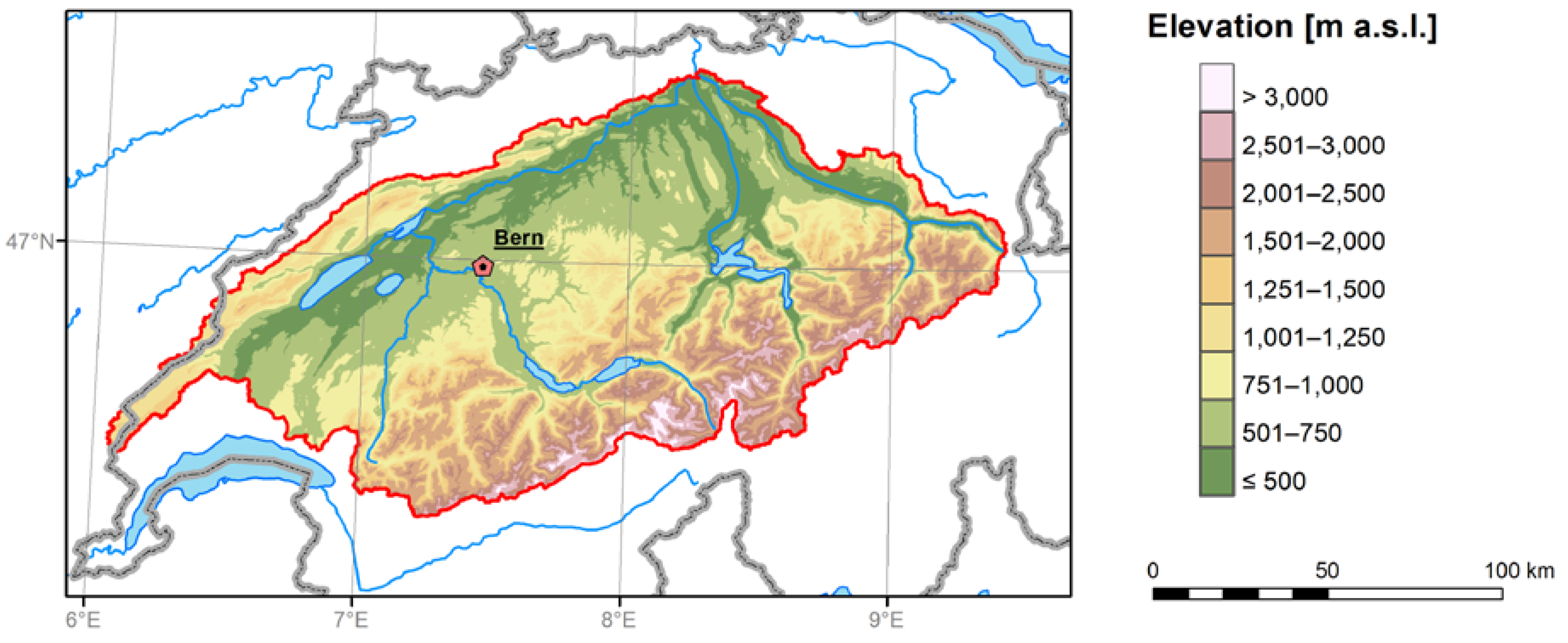
The analysis was performed for the Swiss Plateau and the northern slope of the Swiss Alps. The EXAR data set [21,22] used was originally produced in the context of a hydrological project ‘Assessment of Extreme Flood Risks along the Aare and Rhine rivers’ and refers to the Aare river catchment, covering an area of approximately 17,000 km2 (Figure 1). The data set contains bias-corrected temperature and precipitation series at daily resolution (for both past climate and future scenarios), representing averages for the domain. Thus, no spatial information is present in the data. The observational reference for a bias correction of reanalyses and climate models listed in the EXAR data set was the daily temperature average of 11 stations (Chaumont, Neuchâtel, Château-d’Oex, Bern, Meiringen, Grimsel Hospiz, Andermatt, Altdorf, Luzern, Zurich, and Elm) from the MeteoSwiss network [23]. The bias correction was performed using the quantile mapping technique. In this approach, the climate model simulations are corrected to fit the cumulative distribution of the observational reference [24]. Each individual simulation is corrected separately. As model biases depend on the season [25], a time-dependent correction, calibrated for each calendar day using a 91-day moving window centred at the day of interest was applied. Values below the 1st percentile (or above the 99th percentile) were corrected with the same correction as the 1st (99th) percentile. The cumulative distributions and correction functions for the 15 climate models’ simulations (an example for the low concentration RCP 4.5 scenario) are given in Figure S1. The aforementioned observational reference for bias correction was also used as a source of station data in our study.
Overall, 32 temperature series were obtained from the EXAR data set (1 representing station data, 1 reanalysis, and 30 climate model simulations). The station data series cover the 1900–2014 period. In order to extend the analysis back prior to the 20th century, the bias-corrected 20th Century Reanalysis (version 2c, hereafter referred to as 20CRv2) [26] was used. Although 56 ensemble members of this reanalysis are available for the 1851–2011 period in EXAR, we used only its ensemble mean in the study. For projections of future frost events, two ensembles of bias-corrected regional climate models (RCMs) enlisted in EXAR were used: (i) high-resolution EURO-CORDEX [27] RCM simulations (0.11° grid) driven by global climate models forced by the Representative Concentration Pathway (RCP) 4.5 scenario and ii) the same RCM × GCM ensemble forced by RCP 8.5. In both cases, the lateral boundary conditions were taken from CMIP5 global climate model simulations [28], using observed greenhouse gas concentrations in the 1971–2005 period and the corresponding scenarios in the 2006–2099 period.
The RCP 4.5 scenario represents stabilization of greenhouse gas concentrations without overshooting effective radiative forcing of 4.5 W/m2 relative to pre-industrial values (~650 ppm CO2 equivalent). This is achieved by implementing mitigation policies [29]. By contrast, the RCP 8.5 scenario represents a long-term large energy demand without implementation of mitigation policies, thus leading to high greenhouse gas emissions [30]. This scenario is presumed to reach an effective radiative forcing of 8.5 W/m2 (~1370 ppm CO2 equivalent). Individual ensemble members are listed in Table 1, and they are available for the 1971–2099 period.
2.2. Definition of Spring Frost
A key challenge is to determine whether a frost event occurred after an onset of spring plant growth, at which point plants become vulnerable to temperatures below 0 °C. Although it is possible to use observed vegetation phases from phenological data sets, this procedure cannot be applied into simulated data where the state of vegetation is simplified (in case of climate models) or contain many uncertainties (regarding variety of plant and soil physiological processes simulated by vegetation models). In order to overcome this issue, we proposed a methodology for estimating the beginning of an onset of spring plant growth (hereafter simply called ‘start of spring’) that is based solely on daily mean temperature (TAS) data.
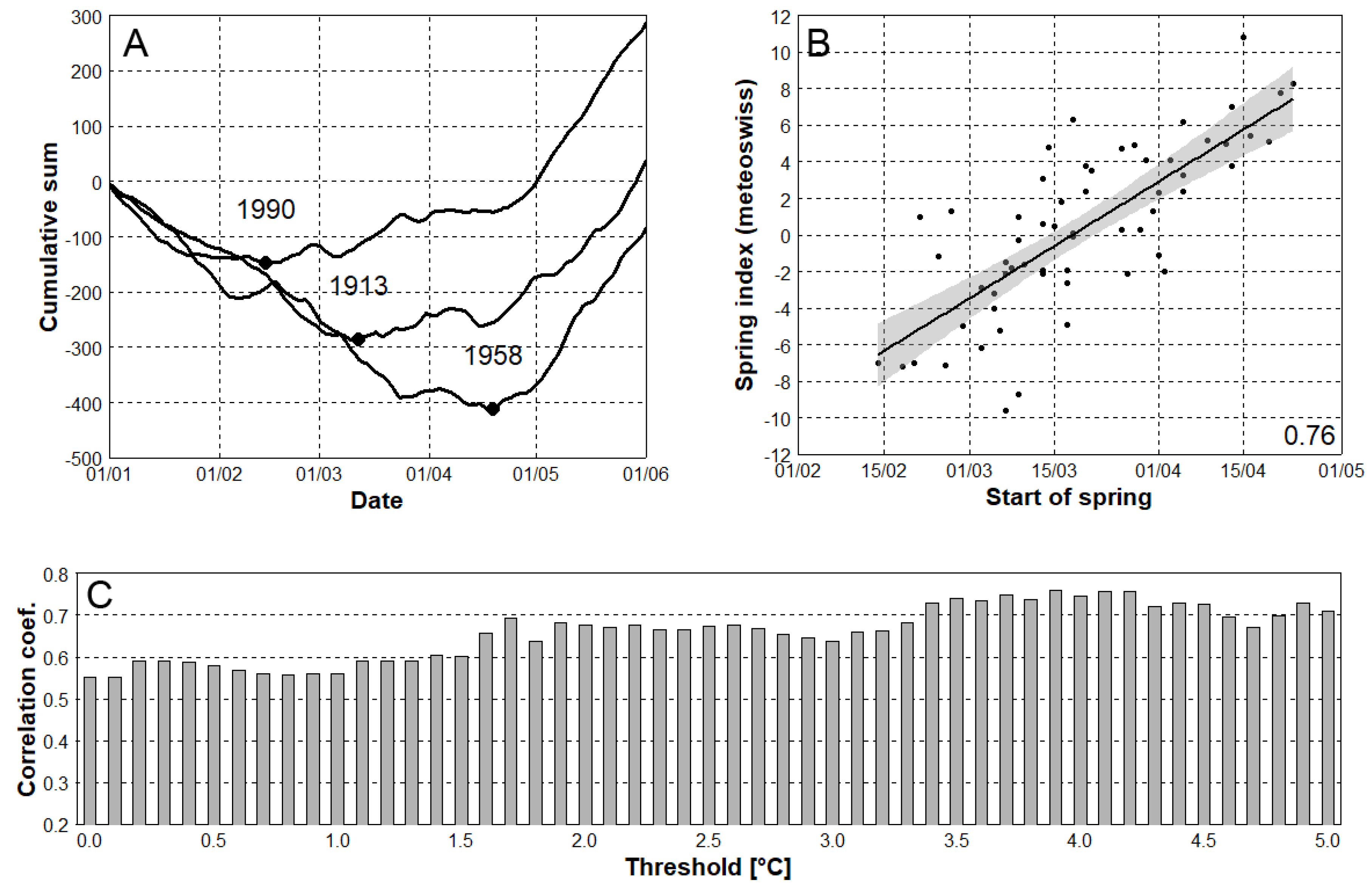
The methodology is similar to a traditional growing degree days approach [32] but it was modified in several key points due to the nature of the study. Because our research domain (Figure 1) consists of various vegetation zones, it is impossible to use predefined species-dependent base temperatures and thermal times required for a calculation of growing degree days [33]. For each year (from January 1 to June 30), a cumulative sum function of TAS anomalies from a selected threshold was calculated. In contrast to a traditional growing degree days approach, negative TAS anomalies are also used (an example for three selected years is given in Figure 2A).
In order to choose the most suitable TAS threshold for the whole domain, its selection was based on a best fit of station data to the Swiss spring index (Figure 2B), which was calculated from in-situ observations of the Swiss Phenology Network [34] (see Brugnara et al. 2020). It is based on the blooming dates (hazel bush, coltsfoot, wood anemone, cherry tree, dandelion, lady’s smock), new leaf formation (horse chestnut tree, hazel bush, beech tree) and new needle formation of the larch [20]. The first principal component is then used to determine the dimensionless deviation of start of spring from the long-term mean. Positive values of spring index indicate that spring vegetation developed later than expected based on the 1981–2010 average, while negative values show earlier vegetation development. TAS threshold values from 0.0 to 5.0 °C were tested for the overlapping 1951–2014 period, and the highest Pearson’s correlation coefficient (0.76) was related to the 3.9 °C threshold (Figure 2C). This threshold value was applied into all series analysed. The start of spring was defined as a date one day after the absolute minimum of the cumulative sum function (Figure 2A). Using the absolute minima of the cumulative sum functions, the method is robust against short term episodes of TAS above the selected threshold.
The severity of spring frost events was analysed using the frost index. The frost index was calculated for each year as a sum of negative TAS anomalies from 0 °C (in absolute values) that occurred after the respective start of spring until June 30 (the rest of the year was excluded due to autumn and winter frosts). Although frost resistance varies among individual species and depends on their phenological phase [2,35], the 0 °C TAS threshold serves as a natural limit for identifying severe spring frost (note that a TAS value of 0 °C may be linked to relatively harsh night-time frosts).
2.3. Other Characteristics and Statistical Testing
Statistical significance of estimated trends was assessed using the non-parametric Mann–Kendal test. A two-sample Student’s t-test was applied for analysing differences in the start of spring between years with spring frost and frost-free springs and for assessing significance of advancements in start of spring between the historical climate and future periods. Finally, a paired Student’s t-test was used for analysing differences between spring dates in station data and 20CRv2.
3. Results
3.1. Evaluation of EXAR Dataset
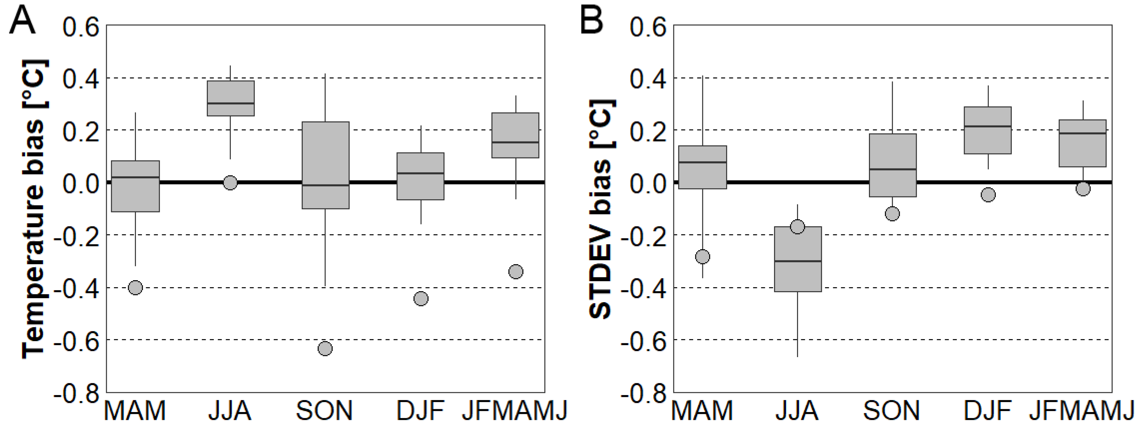
In order to assess creditability of the EXAR dataset, seasonal TAS and its standard deviation from the bias-corrected 20CRv2 reanalysis and the CORDEX RCMs were evaluated against station data in the 1971–2000 period. The 15-member CORDEX ensemble performed well except for summer, when all simulations had a positive TAS bias ranging from 0.1 to 0.4 °C. For the 6 month period in the first half of the year (JFMAMJ, essential for the spring frost analysis), CORDEX tended to have a relatively small positive TAS bias, while a negative bias was found in 20CRv2. Overall, seasonal TAS was systematically lower in 20CRv2 compared to CORDEX (Figure 3A), which may be related to a combination of coarse resolution of original data and complex topography in the analysed domain (Section 2.1). CORDEX RCMs overestimated standard deviations of TAS (STDEV) in all seasons except summer, while standard deviation in 20CRv2 was smaller compared to station data through the year (especially in spring, Figure 3B). A higher (lower) value of STDEV in spring might be associated with more (less) severe frost events.
By applying the 3.9 °C threshold to all series used (Section 2.2), the overestimated TAS in JFMAMJ (Figure 3A) may result in earlier start of spring in CORDEX compared to station data. By contrast, the negative TAS bias found in 20CRv2 may result in later start of spring. The TAS bias was, however, relatively small (ranging from −0.3 to +0.3 °C), and modifying the threshold in accordance with bias values will not substantially improve the link between calculated starts of spring and spring indices in these data sets (considering correlation coefficients, Figure 2C). Moreover, it will have only a small effect on spring frost characteristics (Figure S2).
3.2. Spring Frost in the Historical Climate
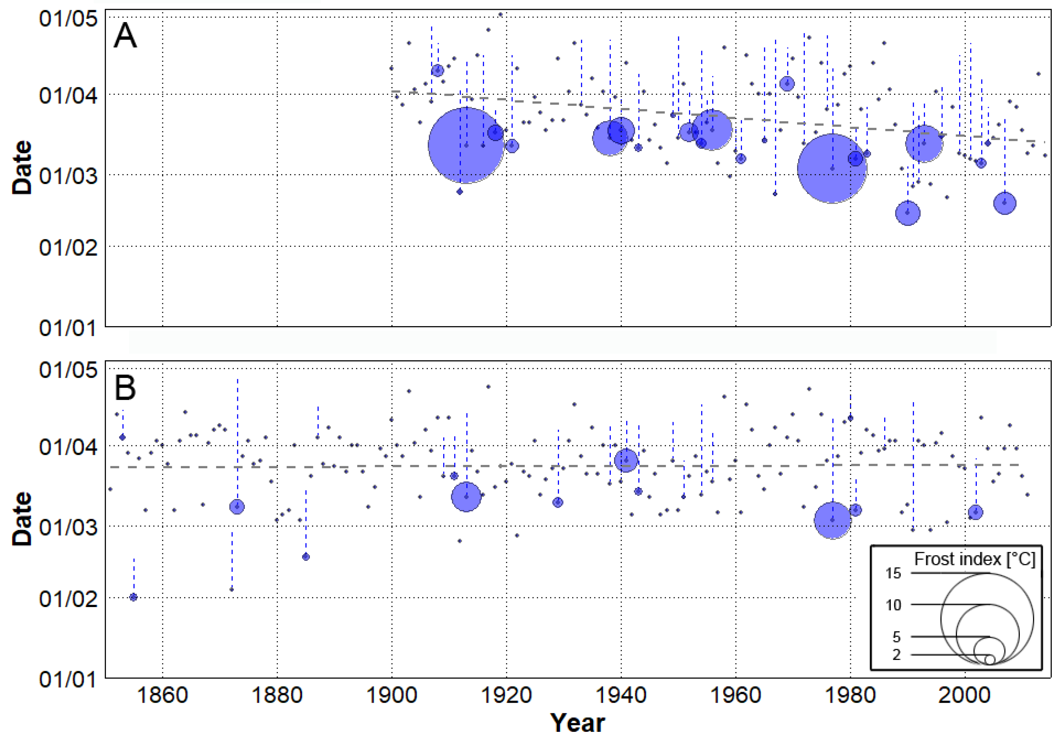
In the station data (1900–2014), the start of spring tended to advance towards the beginning of the calendar year with a significant (at 1% level) trend of 1.8 days/decade. The earliest start of spring (February 14) was recorded in 1990, while the latest end of winter was observed in 1919 when the spring began on May 2. Springs that started earlier were more prone to frost events, as spring frost was present during 37 out of 115 years (approximately every third year), and in those years, springs started significantly (at 1% level) earlier compared to frost-free springs. The most severe spring frost (frost index = 12.2 °C) was observed in April 1913, approximately 1 month after the start of spring and an analogous event occurred in 1977 (Figure 4A). No clear trend of spring frost severity (analysed using frost index) was found in the station data.
In order to assess spring characteristics also in a period prior to the 20th century, a temperature series from 20CRv2 was analysed (Figure 4B). Two extremely early beginnings of spring were found in 1855 and 1872, and both of them were accompanied by a frost event. Overall, no significant differences in starts of spring between the station data and 20CRv2 were found, but 20CRv2 was unable to reproduce a significant advancement of spring starts towards the beginning of the year (considering the overlapping 1900–2011 period). Analogously to the station data, springs that started earlier in the 20CRv2 were significantly (at 1% level) more prone to frost events but their severity was considerably smaller. This may be linked to the negative STDEV bias in 20CRv2 for the spring season (Figure 3B), indicating smaller TAS fluctuations that are essential for frost events.
For an evaluation of CORDEX RCMs, spring characteristics in the relatively recent overlapping 1971–2000 period were calculated. In this period, average dates for start of spring in the station data versus 20CRv2 were March 20 and March 25, respectively. This relatively large difference (with respect to no significant differences in starts of spring between the station data and 20CRv2 in the 1900–2011 period) is linked to much more pronounced advancement of the spring start in the station data (–9.3 days/decade) compared to 20CRv2 (–3.6 days/decade) in 1971–2000. The sum of the yearly frost indices for 1971–2000 (used for RCMs’ evaluation) was 25.8 °C for station data and 9.0 °C for 20CRv2.
3.3. Future Changes of Spring Frost Risk
Because the springs that started earlier had significantly larger abundance of spring frost in the historical climate (Section 3.1), we tested continuity of this relationship in the warming world using simulated data. In the 1971–2000 period, the average date of spring start in the bias-corrected RCMs was in accordance with the station data and varied from March 17 (MPI-REMO-MPI-r2) to March 25 (SMHI-RCA-ICHEC, Table 2). Larger differences between RCMs were found in the sum of the yearly frost indices (ranging from 9.0 to 40.1 °C), but the ensemble mean was still close to the station data.
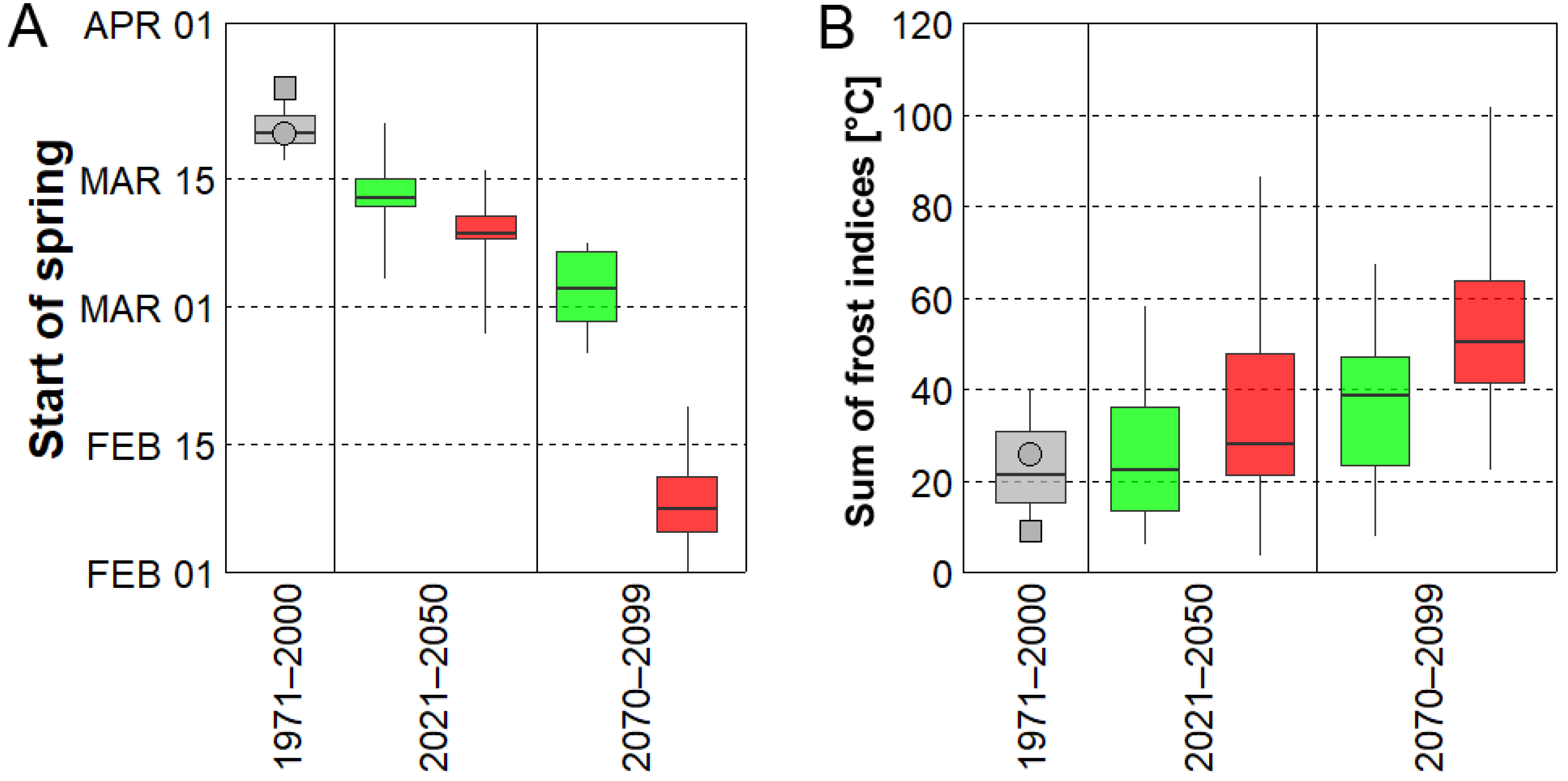
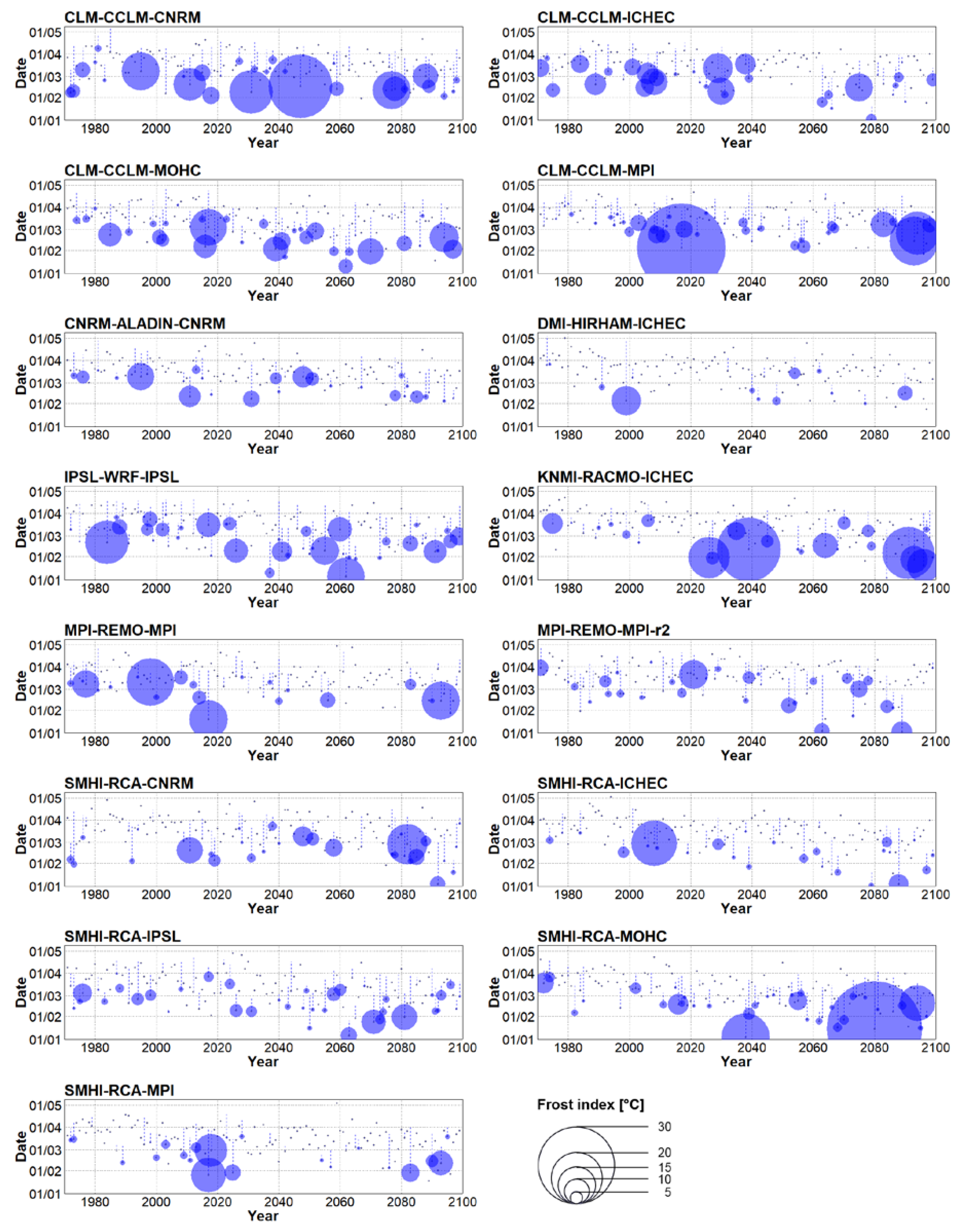
In the near future (2021–2050), spring tends to begin earlier in 13 out of 15 RCMs considering the RCP 4.5 concentration pathway and in all RCMs under RCP 8.5. Those changes are particularly significant under RCP 8.5 (Table 2). On average, the start of spring advances by 8 days under the RCP 4.5 scenario and by 12 days considering RCP 8.5. Inter-model spread was larger compared to the historical period (Figure 5A), and one ensemble member (SMHI-RCA-MOHC forced by RCP 8.5) shifted the average start of spring even to the end of February. The overall advancement of spring’s start was related to larger sums of the yearly frost indices (Figure 5B). In general, the sum of the yearly frost indices increased by a factor of 1.6 under RCP 8.5, and a slightly smaller increment (1.3) was simulated under RCP 4.5. This behaviour was model-dependent, however, because 5 out of 15 RCMs in both concentration scenarios simulated a decline of the frost index. In addition, the link between early (late) start of spring and high (low) frost index was not coherent in some RCMs. For example, the largest sum of the yearly frost indices (86.5 °C in IPSL-WRF-IPS under RCP 8.5) was associated with a rather typical average date for spring’s start for the 2021–2050 period. Moreover, the average starts of spring in KNMI-RACMO-ICHEC were identical in both concentration pathways, but the yearly sums of the frost indices differed substantially (Table 2). It should be noted, however, that these discrepancies might be linked to data sampling, because a severe frost event may occur outside the 30-year-long analysed periods (e.g., an exceptional frost event in model year 2017 simulated by CLM-CCLM-MPI forced by RCP 4.5, Figure 6).
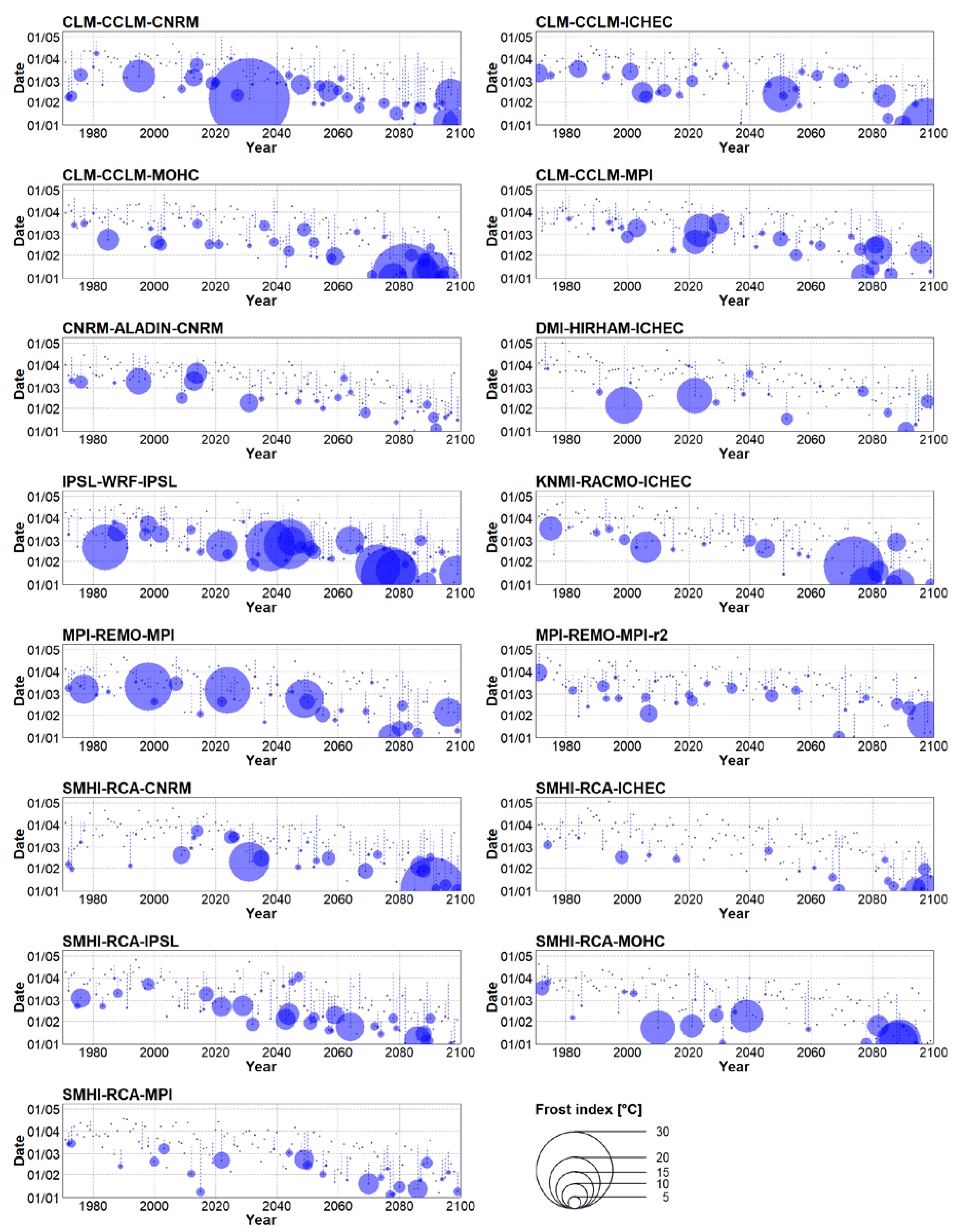
Additional shifts of the average start of spring towards the beginning of the year were simulated for the end of the 21st century (2070–2099). Under the RCP 4.5 concentration scenario, spring started nearly 3 weeks earlier on average compared to the historical period and a substantial statistically significant advancement in the start of spring was simulated under RCP 8.5 (Table 2, Figure 5A). At the end of the 21st century, many RCMs simulated springs that start right after the beginning of the year, meaning that winter (by our definition) ends before the close of the year or does not occur at all (Figure 6 and Figure 7). Considering the RCP 8.5 scenario, all RCMs simulated higher values of the sums of the yearly frost indices with respect to their historical runs. The ensemble mean’s sum of the yearly frost indices was larger by a factor of 2.9 compared to the station data and the increment was projected by 13 out of 15 RCMs (the two remaining RCM had values comparable to station data, Table 2). When forced by RCP 4.5, the RCMs simulated a smaller increase in the 2070–2099 period (2.0) compared to RCP 8.5.
4. Discussion
Projecting changes in vegetation responses to a possible future climate is a challenging task that is accompanied by many uncertainties. The proposed method aims to provide a robust approach for assessing future spring frost risk for the complex Swiss terrain that contains several different vegetation zones, based on a widely available daily mean temperature only. The method was calibrated in 1951–2014 using the Swiss spring index constructed from phenological in-situ observation [34]; however, it is possible that the relationship between temperature characteristics in spring and timing of vegetation’s development would be changed in the future climate [36] because this link is probably not linear [37]. Many authors reported that climate change is responsible for decreased temperature sensibility of bud break. For example, Wang et al. [38] suggested that plants might be less likely to track climatic warming at locations with larger local spring temperature variance in order to avoid a frost risk and rely more on other cues, such as high chill requirements or photoperiods.
The 3.9 °C threshold value used in our method for identifying starts of spring corresponds to the growth-onset temperature identified by Breitenmoser et al. [39] for mid-latitudinal trees, however, it has to be considered that the threshold value represents an average over the whole analysed domain. Therefore, the threshold value has to be regarded with caution, because it may vary between vegetation zones [15]. Due to the size of the domain and its terrain heterogeneity, we employed daily mean temperature instead of commonly used daily minimum temperature when calculating the frost index. Low night-time temperature minima are often linked to geomorphologic features, such as altitude, shape of valleys, or exposition of slopes and may differ substantially between nearby locations [40,41]. The use of spatially more coherent daily mean temperature allows distinguishing of larger-scale frost events that are mostly related to an interruption of the prevailing westerly flow [42] and an incursion of a cold air mass from northern or eastern directions [43]. Cold northerly/easterly advection into Central and Western Europe is often linked to blocking anticyclones [44].
Improper simulation of frequency and persistence of blocking anticyclones is one of the largest drawbacks of current climate models [45,46], and it influences projections of circulation-induced temperature and precipitation extremes in a future climate [47]. Furthermore, Lhotka and Kyselý [48] showed that climate models tend to have too-cold northerly advection in winter, and this deficiency may propagate also into a spring season. Although the RCMs used simulated the spring frost index relatively well in the historical climate, an analysis of frost events’ driving mechanisms is beyond the scope of this study. The 20CRv2 reanalysis did not capture the observed advancement of the spring start towards the beginning of the year, and the average date of spring start differed by 5 days compared to the observed data (considering the 1971–2000 period). Lorenz and Jacob [49] found weaker temperature trends in the NCEP/NCAR reanalysis over Europe compared to E-OBS and CRU observed data sets. Inasmuch as the 20CRv2 reanalysis shares many features with the NCEP/NCAR reanalysis [26,50], the erroneous, weaker temperature trend is probably present also in 20CRv2, and it is most likely related to this discrepancy.
Although substantial progress has been made in understanding relationships between increasing temperatures and shifts of phenophases, exact physiological mechanisms are still a subject of broad discussions. Cong et al. [51] reported that interannual variations in an onset of spring plant growth are extensively related to the number of chilling days over the Tibetan Plateau and suggested that continued future warming may lead to a deficiency in chilling and thus in changes in phenophase timing. An analogous phenomenon was reported in Switzerland by Asse et al. [52], who concluded that warmer winters significantly delayed bud burst and flowering along the elevation gradient. The role of a chill requirement, however, was questioned by Güsewell et al. [53], who found that reduced temperature sensitivity can result directly from spring warming alone. In addition, the importance of photoperiods for spring phenophases is not clear, and their roles are probably species- and region-dependent [54,55]. Another important factor is a timing of snowmelt, especially in regions with higher elevation [56]. Finally, besides spring frost risk, other hazards such as heat waves and droughts or spread of pests [57] should be taken into account when preparing complex climate change adaptation and mitigation strategies.
5. Conclusions
Using 15 bias-corrected CORDEX RCMs from the EXAR data set, changes in characteristics of spring frost in Switzerland under climate change were analysed. The main conclusions can be summarized as follows:
- The methodology for estimating an onset of spring plant growth solely from temperature data was developed and tested. The estimated dates were well correlated (correlation coefficient = 0.76) with the Swiss spring index that was calculated from actual phenological observations.
- Significant (at 1% level) advancement of spring start was found in the observed data, with a trend of 1.8 days/decade in the 1900–2014 period. The 20CRv2 reanalysis failed to reproduce this trend.
- In the observed data, springs with early start were significantly (at 1% level) more prone to experience frost events compared to spring that began later. This relationship was, in general, simulated also in a future climate, but in some RCMs, a substantial spring advancement was not linked to a large sum of the yearly frost indices and vice versa.
- Considering the 2021–2050 period, spring is projected to start 8 or 12 days earlier (depending on concentration scenario). This advancement is linked to larger sums of the yearly frost indices compared to historical climate, approximately by a factor of 1.3 or 1.6, respectively.
- Major differences between concentration scenarios were found at the end of the 21st century (2070–2099). The earliest starts of spring and the largest values of the sum of yearly frost indices were simulated under RCP 8.5, in which the mean date of spring start was February 9 (about 6 weeks earlier) and the sum of the yearly frost indices was larger by a factor of 2.9 compared to historical climate.
Overall, we conclude that frost risk after an onset of spring plant growth will be larger in a future climate of Switzerland under both ‘low’ and ‘high’ concentration scenarios. The risk might be reduced by vegetation’s adaptation mechanisms and changes in physiological processes, as discussed above, but it is questionable whether plants can adapt fast enough to follow the unprecedented (at least within the past several thousand years) warming trend projected under the RCP 8.5 concentration pathway. Further improvement may be associated with an analysis of regional patterns using the new CH2018 Swiss climate scenarios [58], which will allow for determining future frost risk on a 2 × 2 km grid.
Supplementary Materials
The following are available online at https://www.mdpi.com/2073-4433/11/4/391/s1, Figure S1: Cumulative distributions of daily mean temperature and correction functions for 15 climate model simulations and Figure S2: Interannual variability in starts of spring calculated for the bias-corrected 20th Century Reanalysis using two different thresholds.
Author Contributions
Conceptualization, S.B.; Investigation, O.L.; Methodology, O.L.; Supervision, S.B.; Visualization, O.L.; Writing—Original draft, O.L.; Writing—Review & editing, S.B. All authors have read and agreed to the published version of the manuscript.
Funding
The study was supported by the Czech Science Foundation, project 20-28560S. Ondřej Lhotka contribution was also supported by the project SustES—Adaptation strategies for sustainable ecosystem services and food security under adverse environmental conditions (CZ.02.1.01/0.0/0.0/16_019/0000797).
Acknowledgments
The project EXAR—Understanding Extreme Flooding Events Aare-Rhein in Switzerland—was funded by the Swiss Federal Office for the Environment (FOEN), the Swiss Federal Office of Energy (SFOE), and the Swiss Federal Nuclear Safety Inspectorate (ENSI). We acknowledge the World Climate Research Programme’s Working Group on Regional Climate and the Working Group on Coupled Modelling, former coordinating body of CORDEX and responsible panel for CMIP5.
Conflicts of Interest
The authors declare no conflict of interest and the funders had no role in the design of the study; in the collection, analyses, or interpretation of data; in the writing of the manuscript, or in the decision to publish the results.
References
- Kollas, C.; Körner, C.; Randin, C.F. Spring frost and growing season length co-control the cold range limits of broad-leaved trees. J. Biogeogr. 2014, 41, 773–783. [Google Scholar] [CrossRef]
- Meier, M.; Fuhrer, J.; Holzkämper, A. Changing risk of spring frost damage in grapevines due to climate change? A case study in the Swiss Rhone Valley. Int. J. Biometeorol. 2018, 62, 991–1002. [Google Scholar] [CrossRef] [PubMed] [Green Version]
- Vitasse, Y.; Rebetez, M. Unprecedented risk of spring frost damage in Switzerland and Germany in 2017. Clim. Chang. 2018, 149, 233–246. [Google Scholar] [CrossRef]
- Augspurger, C.K. Reconstructing patterns of temperature, phenology, and frost damage over 124 years: Spring damage risk is increasing. Ecology 2013, 94, 41–50. [Google Scholar] [CrossRef] [PubMed]
- Jeong, S.-J.; Ho, C.-H.; Gim, H.-J.; Brown, M.E. Phenology shifts at start vs. end of growing season in temperate vegetation over the Northern Hemisphere for the period 1982–2008. Glob. Chang. Biol. 2011, 17, 2385–2399. [Google Scholar] [CrossRef]
- Menzel, A.; Sparks, T.H.; Estrella, N.; Koch, E.; Aasa, A.; Ahas, R.; Alm-Kübler, K.; Bissolli, P.; Braslavská, O.; Briede, A.; et al. European phenological response to climate change matches the warming pattern. Glob. Chang. Biol. 2006, 12, 1969–1976. [Google Scholar] [CrossRef]
- Lavalle, C.; Micale, F.; Houston, T.D.; Camia, A.; Hiederer, R.; Lazar, C.; Costanza, C.; Amatulli, G.; Genovese, G. Climate change in Europe. 3. Impact on agriculture and forestry. A review. Agron. Sustain. Dev. 2009, 29, 433–446. [Google Scholar] [CrossRef] [Green Version]
- Shen, M.; Cong, N.; Cao, R. Temperature sensitivity as an explanation of the latitudinal pattern of green-up date trend in Northern Hemisphere vegetation during 1982–2008. Int. J. Climatol. 2015, 35, 3707–3712. [Google Scholar] [CrossRef]
- Kolářová, E.; Nekovář, J.; Adamík, P. Long-term temporal changes in central European tree phenology (1946−2010) confirm the recent extension of growing seasons. Int. J. Biometeorol. 2014, 58, 1739–1748. [Google Scholar] [CrossRef]
- Legave, J.M.; Blanke, M.; Christen, D.; Giovannini, D.; Mathieu, V.; Oger, R. A comprehensive overview of the spatial and temporal variability of apple bud dormancy release and blooming phenology in Western Europe. Int. J. Biometeorol. 2013, 57, 317–331. [Google Scholar] [CrossRef]
- Wypych, A.; Ustrnul, Z.; Sulikowska, A.; Chmielewski, F.-M.; Bochenek, B. Spatial and temporal variability of the frost-free season in Central Europe and its circulation background. Int. J. Climatol. 2017, 37, 3340–3352. [Google Scholar] [CrossRef]
- Bigler, C.; Bugmann, H. Climate-induced shifts in leaf unfolding and frost risk of European trees and shrubs. Sci. Rep. 2018, 9865. [Google Scholar] [CrossRef] [PubMed] [Green Version]
- Liu, Q.; Piao, S.; Janssens, I.M.; Fu, Y.; Peng, S.; Lian, X.; Ciais, P.; Myneni, R.B.; Penuelas, J.; Wang, T. Extension of the growing season increases vegetation exposure to frost. Nat. Commun. 2018, 9. [Google Scholar] [CrossRef] [PubMed] [Green Version]
- Kim, Y.; Kimball, J.S.; Didan, K.; Henebry, G.M. Response of vegetation growth and productivity to spring climate indicators in the conterminous United States derived from satellite remote sensing data fusion. Agric. For. Meteorol. 2014, 194, 132–143. [Google Scholar] [CrossRef]
- Vitasse, Y.; Schneider, L.; Rixen, C.; Christen, D.; Rebetez, M. Increase in the risk of exposure of forest and fruit trees to spring frosts at higher elevations in Switzerland over the last four decades. Agric. For. Meteorol. 2018, 248, 60–69. [Google Scholar] [CrossRef]
- Bennie, J.; Kubin, E.; Wiltshire, A.; Huntley, B.; Baxter, R. Predicting spatial and temporal patterns of bud-burst and spring frost risk in north-west Europe: The implications of local adaptation to climate. Glob. Chang. Biol. 2010, 16, 1503–1514. [Google Scholar] [CrossRef]
- Molitor, D.; Caffarra, A.; Sinigoj, P.; Pertot, I.; Hoffmann, L.; Junk, J. Late frost damage risk for viticulture under future climate conditions: A case study for the Luxembourgish winegrowing region. Aust. J. Grape Wine Res. 2014, 20, 160–168. [Google Scholar] [CrossRef]
- Leolini, L.; Moriondo, M.; Fila, G.; Costafreda-Aumedes, S.; Ferrise, R.; Bindi, M. Late spring frost impacts on future grapevine distribution in Europe. Field Crop. Res. 2018, 222, 197–208. [Google Scholar] [CrossRef]
- Mosedale, J.R.; Wilson, R.J.; Maclean, I.M. Climate Change and Crop Exposure to Adverse Weather: Changes to Frost Risk and Grapevine Flowering Conditions. PLoS ONE 2015. [Google Scholar] [CrossRef] [Green Version]
- Spring Index. Available online: https://www.meteoswiss.admin.ch/home/climate/climate-change-in-switzerland/vegetation-development/spring-index.html (accessed on 12 October 2019).
- Brönnimann, S.; Rajczak, J.; Fischer, E.M.; Raible, C.C.; Rohrer, M.; Schär, C. Changing seasonality of moderate and extreme precipitation events in the Alps. Nat. Hazard. Earth Syst. 2018, 18, 2047–2056. [Google Scholar] [CrossRef] [Green Version]
- Rajczak, J.; Brönnimann, S.; Fischer, E.M.; Raible, C.C.; Rohrer, M.; Schär, C. Daily Precipitation and Temperature Time Series from Multiple Climate Model Simulations for the Aare River Catchment (Switzerland). Available online: https://www.pangaea.de (accessed on 12 October 2019). [CrossRef]
- Begert, M.; Schlegel, T.; Kirchhofer, W. Homogeneous Temperature and Precipitation Series of Switzerland from 1864 to 2000. Int. J. Climatol. 2005, 25, 65–80. [Google Scholar] [CrossRef]
- Maraun, D. Bias Correction, Quantile Mapping, and Downscaling: Revisiting the Inflation Issue. J. Clim. 2013, 26, 2137–2143. [Google Scholar] [CrossRef] [Green Version]
- Rajczak, J.; Schär, C. Projections of Future Precipitation Extremes Over Europe: A Multimodel Assessment of Climate Simulations. J. Geophys. Res. Atmos. 2017, 122, 10–773. [Google Scholar] [CrossRef]
- Compo, G.P.; Whitaker, J.S.; Sardeshmukh, P.D.; Matsui, N.; Allan, R.J.; Yin, X.; Gleason, B.E.; Vose, R.S.; Rutledge, G.; Bessemoulin, P.; et al. The Twentieth Century Reanalysis Project. Q. J. R. Meteorol. Soc. 2011, 137, 1–28. [Google Scholar] [CrossRef]
- Jacob, D.; Petersen, J.; Eggert, B.; Alias, A.; Christensen, O.B.; Bouwer, L.M.; Braun, A.; Colette, A.; Déqué, M.; Georgievski, G.; et al. EURO-CORDEX: New high-resolution climate change projections for European impact research. Reg. Environ. Chang. 2014, 14, 563–578. [Google Scholar] [CrossRef]
- Taylor, K.E.; Stouffer, R.J.; Meehl, G.A. An overview of CMIP5 and the experiment design. Bull. Am. Meteorol. Soc. 2012, 93, 485–498. [Google Scholar] [CrossRef] [Green Version]
- Thomson, A.M.; Calvin, K.V.; Smith, S.J.; Kyle, G.P.; Volke, A.; Patel, P.; Delgado-Arias, S.; Bond-Lamberty, B.; Wise, M.A.; Clarke, L.E.; et al. RCP 4.5: A pathway for stabilization of radiative forcing by 2100. Clim. Chang. 2011, 109, 77–94. [Google Scholar] [CrossRef] [Green Version]
- Riahi, K.; Rao, S.; Krey, V.; Cho, C.; Chirkov, V.; Fischer, G.; Nakicenovic, N.; Rafaj, P. RCP 8.5—A scenario of comparatively high greenhouse gas emissions. Clim. Chang. 2011, 109, 33–57. [Google Scholar] [CrossRef] [Green Version]
- Kotlarski, S.; Keuler, K.; Christensen, O.B.; Colette, A.; Déqué, M.; Gobiet, A.; Goergen, K.; Jacob, D.; Lüthi, D.; van Meijgaard, E.; et al. Regional climate modeling on European scales: A joint standard evaluation of the EURO-CORDEX RCM ensemble. Geosci. Model. Dev. 2014, 7, 1297–1333. [Google Scholar] [CrossRef] [Green Version]
- McMaster, G.S.; Wilhelm, W.W. Growing degree-days: One equation, two interpretations. Agric. For. Meteorol. 1997, 87, 291–300. [Google Scholar] [CrossRef] [Green Version]
- Campbell, G.S.; Norman, J. An Introduction to Environmental Biophysics; Springer: New York, NY, USA, 1998; p. 286. ISBN 978-0-387-94937-6. [Google Scholar]
- Brugnara, Y.; Auchmann, R.; Rutishauser, T.; Gehrig, R.; Pietragalla, B.; Begert, M.; Sigg, C.; Knechtl, V.; Konzelmann, T.; Calpini, B.; et al. Homogeneity assessment of phenological records from the Swiss Phenology Network. Int. J. Biometeorol. 2020, 64, 71–81. [Google Scholar] [CrossRef] [PubMed]
- Venn, S.E.; Green, K. Evergreen alpine shrubs have high freezing resistance in spring, irrespective of snowmelt timing and exposure to frost: An investigation from the Snowy Mountains, Australia. Plant Ecol. 2017, 219, 209–216. [Google Scholar] [CrossRef]
- Richardson, A.D.; Keenan, T.F.; Migliavacca, M.; Ryu, Y.; Sonnentag, O.; Toomey, M. Climate change, phenology, and phenological control of vegetation feedbacks to the climate system. Agric. For. Meteorol. 2013, 169, 156–173. [Google Scholar] [CrossRef]
- Eccel, E.; Rea, R.; Caffarra, A.; Crisci, A. Risk of spring frost to apple production under future climate scenarios: The role of phenological acclimation. Int. J. Biometeorol. 2009, 53, 273–286. [Google Scholar] [CrossRef]
- Wang, T.; Ottlé, C.; Peng, S.; Janssens, I.A.; Lin, X.; Poulter, B.; Yue, C.; Ciais, P. The influence of local spring temperature variance on temperature sensitivity of spring phenology. Glob. Chang. Biol. 2014, 20, 1473–1480. [Google Scholar] [CrossRef] [PubMed]
- Breitenmoser, P.; Brönnimann, S.; Frank, D. Forward modelling of tree-ring width and comparison with a global network of tree-ring chronologies. Clim. Past 2014, 10, 437–449. [Google Scholar] [CrossRef] [Green Version]
- Kleiber, W.; Katz, R.W.; Rajagopalan, B. Daily minimum and maximum temperature simulation over complex terrain. Ann. Appl. Stat. 2013, 7, 588–612. [Google Scholar] [CrossRef] [Green Version]
- Giaccone, E.; Luoto, M.; Vittoz, P.; Guisan, A.; Mariéthoz, G.; Lambiel, C. Influence of microclimate and geomorphological factors on alpine vegetation in the Western Swiss Alps. Earth Surf. Process. Landf. 2019, 44, 3093–3107. [Google Scholar] [CrossRef] [Green Version]
- Cattiaux, J.; Yiou, P.; Vautard, R. Dynamics of future seasonal temperature trends and extremes in Europe: A multi-model analysis from CMIP3. Clim. Dynam. 2012, 38, 1949–1964. [Google Scholar] [CrossRef]
- Ustrnul, Z.; Wypych, A.; Winkler, J.A.; Czekierda, D. Late Spring Freezes in Poland in Relation to Atmospheric Circulation. QuaGeo 2014, 33, 165–172. [Google Scholar] [CrossRef] [Green Version]
- Yao, Y.; Luo, D.; Dai, A.; Simmonds, I. Increased quasi stationarity and persistence of winter Ural blocking and Eurasian extreme cold events in response to arctic warming. Part I: Insights from Observational Analyses. J. Clim. 2017, 30, 3569–3587. [Google Scholar] [CrossRef]
- Masato, G. Winter and Summer Northern Hemisphere Blocking in CMIP5 Models. J. Clim. 2013, 26, 7044–7059. [Google Scholar] [CrossRef]
- Dunn-Sigouin, E.; Son, S.-W. Northern Hemisphere blocking frequency and duration in the CMIP5 models. J. Geophys. Res. Atmos. 2013, 118, 1179–1188. [Google Scholar] [CrossRef]
- Scaife, A.A.; Woollings, T.; Knight, J.; Martin, G.; Hinton, T. Atmospheric Blocking and Mean Biases in Climate Models. J. Clim. 2010, 23, 6143–6152. [Google Scholar] [CrossRef] [Green Version]
- Lhotka, O.; Kyselý, J. Circulation-Conditioned Wintertime Temperature Bias in EURO-CORDEX Regional Climate Models over Central Europe. J. Geophys. Res. Atmos. 2018, 16, 8661–8673. [Google Scholar] [CrossRef]
- Lorenz, P.; Jacob, D. Validation of temperature trends in the ENSEMBLES regional climate model runs driven by ERA40. Clim. Res. 2010, 44, 167–177. [Google Scholar] [CrossRef]
- Kalnay, E.; Kanamitsu, M.; Kistler, R.; Collins, W.; Deaven, D.; Gandin, L.; Iredell, M.; Saha, S.; White, G.; Woollen, J.; et al. The NCEP/NCAR 40-year reanalysis project. Bull. Am. Meteorol. Soc. 1996, 77, 437–471. [Google Scholar] [CrossRef] [Green Version]
- Cong, N.; Shen, M.; Piao, S.; Chen, X.; An, S.; Yang, W.; Fu, Y.H.; Meng, F.; Wang, T. Little change in heat requirement for vegetation green-up on the Tibetan Plateau over the warming period of 1998–2012. Agric. For. Meteorol. 2017, 232, 650–658. [Google Scholar] [CrossRef]
- Asse, D.; Chuine, I.; Vitasse, Y.; Yocco, N.G.; Delpierre, N. Warmer winters reduce the advance of tree spring phenology induced by warmer springs in the Alps. Agric. For. Meteorol. 2018, 252, 220–230. [Google Scholar] [CrossRef]
- Güsewell, S.; Furrer, R.; Gehrig, R.; Pietragalla, B. Changes in temperature sensitivity of spring phenology with recent climate warming in Switzerland are related to shifts of the preseason. Glob. Chang. Biol. 2017, 23, 5189–5202. [Google Scholar] [CrossRef]
- Körner, C.; Basler, D. Phenology under Global Warming. Science 2010, 327, 1461–1462. [Google Scholar] [CrossRef] [PubMed]
- Migliavacca, M.; Sonnentag, O.; Keenan, T.F.; Cescatti, A.; O’keefe, J.; Richardson, A.D. On the uncertainty of phenological responses to climate change, and implications for a terrestrial biosphere model. Biogeosciences 2012, 9, 2063–2083. [Google Scholar] [CrossRef] [Green Version]
- Chen, X.; An, S.; Inouye, D.W.; Schwartz, M.D. Temperature and snowfall trigger alpine vegetation green-up on the world’s roof. Glob. Chang. Biol. 2015, 21, 3635–3646. [Google Scholar] [CrossRef] [PubMed]
- Young, S.L. As Climate Shifts, So Do Pests: A National Forum and Assessment. Bull. Ecol. Soc. Am. 2017, 98, 165–172. [Google Scholar] [CrossRef]
- CH2018. CH2018—Climate Scenarios for Switzerland, Technical Report; National Centre for Climate Services: Zürich, Switzerland, 2018; p. 271. ISBN 978-3-9525031-4-0. [Google Scholar]
Figure 1.
Location of study domain (red polygon) within Switzerland. All data used in this study represent averages over this region.
Figure 1.
Location of study domain (red polygon) within Switzerland. All data used in this study represent averages over this region.

Figure 2.
(A) Definition of start of spring; an example for years 1913, 1958, and 1990 using the 3.9 °C threshold. Solid curves represent cumulative sum functions, while black dots indicate starts of spring. (B) Correlation between starts of spring calculated from station data and the MeteoSwiss spring index using the 3.9 °C threshold. Dots indicate individual years, and the number 0.76 is the Pearson’s correlation coefficient. (C) Differences in Pearson’s correlation coefficients when using various threshold values.

Figure 3.
(A) Seasonal temperature bias for 15-member CORDEX ensemble (box plots) and 20th Century Reanalysis version 2c (circles) against station data. (B) Same as Figure 3A but for standard deviation of daily mean temperature. MAM stands for March 1–May 31 period, JJA for June 1–August 31, SON for September 1–November 30, DJF for December 1–February 28 (29) and JFMAMJ for January 1–June 30.

Figure 4.
Interannual variability in starts of spring (grey dots) with their least-squares trends (grey dashed lines) for station data (A) and the bias-corrected 20th Century Reanalysis, version 2c (B). Blue circles highlight springs with frost event(s) and their size indicates the value of frost index. Blue dashed lines represent periods between a start of spring and a last frost event.

Figure 5.
(A) Distributions of average start of spring and (B) sum of yearly frost indices in the historical climate (grey) and two future time periods (2021–2050 and 2070–2099) using individual bias-corrected ensemble members. Green colour represents simulations forced by RCP 4.5, while red colour indicates simulations forced by RCP 8.5. Grey circle stands for station data, while grey square represents the bias-corrected 20th Century Reanalysis, version 2c.

Figure 6.
Interannual variability of spring start dates (grey dots) in individual bias-corrected climate model simulations forced by the RCP 4.5 concentration pathway. Blue circles highlight springs with frost event(s) and their size indicates the value of frost index. Blue dashed lines represent periods between a start of spring and a last frost event.

Figure 7.
Same as Figure 6 but for simulations forced by the RCP 8.5 concentration pathway.
Figure 7.
Same as Figure 6 but for simulations forced by the RCP 8.5 concentration pathway.


Table 1.
Regional climate models (RCMs) driven by global climate models (GCMs) from the EURO-CORDEX project extracted from the EXAR data set. All RCMs originally used the 0.11° rotated grid and are available driven by GCMs, forced by both RCP 4.5 and RCP 8.5 concentration pathways.
Table 1.
Regional climate models (RCMs) driven by global climate models (GCMs) from the EURO-CORDEX project extracted from the EXAR data set. All RCMs originally used the 0.11° rotated grid and are available driven by GCMs, forced by both RCP 4.5 and RCP 8.5 concentration pathways.
| Institute | Acronym | RCM | GCM |
|---|---|---|---|
| Climate Limited-Area Modelling Community | CLM | CCLM | CNRM |
| ICHEC | |||
| MOHC | |||
| MPI | |||
| National Centre for Meteorological Research | CNRM | ALADIN | CNRM |
| Danish Meteorological Institute | DMI | HIRHAM | ICHEC |
| Institute Pierre Simon Laplace | IPSL | WRF | IPSL |
| Royal Netherlands Meteorological Institute | KNMI | RACMO | ICHEC |
| Max Planck Institute for Meteorology | MPI | REMO | MPI* |
| Swedish Meteorological and Hydrological Institute | SMHI | RCA | CNRM |
| HadGEM | |||
| ICHEC | |||
| IPSL | |||
| MPI |
* Two individual runs of MPI-REMO-MPI simulations (r1i1p1 and r2i1p1) were used in the EXAR data set. Detailed information about individual RCMs’ characteristics are provided in Kotlarski et al. [31].
Table 2.
Average start of spring (S) and sum of the yearly frost indices (If) in the bias-corrected regional climate models, station data and 20th Century Reanalysis (version 2c). Three time periods (1971–2000, 2021–2050 and 2070–2099) are considered. Values in parentheses indicate changes (ratios) in sum of frost index compared to the historical period in respective models. Bold values represent statistically significant change at 5% level and bold underlined ones at 1% level compared to the historical period (only starts of spring in individual models in future periods were tested).
| Historical | RCP 4.5 | RCP 8.5 | ||||||||
|---|---|---|---|---|---|---|---|---|---|---|
| 1971–2000 | 2021–2050 | 2070–2099 | 2021–2050 | 2070–2099 | ||||||
| S | If [°C] | S | If [°C] | S | If [°C] | S | If [°C] | S | If [°C] | |
| CLM-CCLM-CNRM | 19/03 | 36.3 | 14/03 | 58.1 (1.6) | 07/03 | 49.6 (1.4) | 11/03 | 54.1 (1.5) | 12/02 | 63.8 (1.8) |
| CLM-CCLM-ICHEC | 19/03 | 33.9 | 12/03 | 40.2 (1.2) | 01/03 | 28.8 (0.8) | 11/03 | 27.9 (0.8) | 18/02 | 50.8 (1.5) |
| CLM-CCLM-MOHC | 20/03 | 22.0 | 07/03 | 35.8 (1.6) | 04/03 | 38.8 (1.8) | 06/03 | 24.2 (1.1) | 01/02 | 101.6 (4.6) |
| CLM-CCLM-MPI | 20/03 | 15.0 | 12/03 | 15.7 (1.0) | 08/03 | 57.4 (3.8) | 10/03 | 46.8 (3.1) | 08/02 | 59.7 (4.0) |
| CNRM-ALADIN-CNRM | 21/03 | 21.1 | 16/03 | 21.1 (1.0) | 03/03 | 17.7 (0.8) | 12/03 | 15.1 (0.7) | 08/02 | 25.6 (1.2) |
| DMI-HIRHAM-ICHEC | 24/03 | 15.4 | 14/03 | 6.1 (0.4) | 07/03 | 7.9 (0.5) | 09/03 | 23.1 (1.5) | 19/02 | 22.5 (1.5) |
| IPSL-WRF-IPSL | 20/03 | 40.1 | 12/03 | 36.5 (0.9) | 03/03 | 40.1 (1.0) | 09/03 | 86.5 (2.2) | 06/02 | 98.4 (2.5) |
| KNMI-RACMO-ICHEC | 23/03 | 16.3 | 09/03 | 58.2 (3.6) | 25/02 | 60.3 (3.7) | 09/03 | 16.3 (1.0) | 06/02 | 75.8 (4.7) |
| MPI-REMO-MPI | 19/03 | 39.5 | 16/03 | 8.7 (0.2) | 07/03 | 22.5 (0.6) | 08/03 | 50.4 (1.3) | 11/02 | 42.7 (1.1) |
| MPI-REMO-MPI-r2 | 17/03 | 23.9 | 21/03 | 23.8 (1.0) | 08/03 | 30.5 (1.3) | 16/03 | 19.6 (0.8) | 17/02 | 33.4 (1.4) |
| SMHI-RCA-CNRM | 18/03 | 10.6 | 18/03 | 19.5 (1.8) | 29/02 | 44.4 (4.2) | 09/03 | 37.5 (3.5) | 08/02 | 63.9 (6.0) |
| SMHI-RCA-ICHEC | 25/03 | 9.0 | 12/03 | 11.1 (1.2) | 25/02 | 21.6 (2.4) | 11/03 | 3.4 (0.4) | 10/02 | 40.3 (4.5) |
| SMHI-RCA-IPSL | 19/03 | 27.6 | 13/03 | 22.2 (0.8) | 28/02 | 43.6 (1.6) | 08/03 | 49.1 (1.8) | 02/02 | 43.0 (1.6) |
| SMHI-RCA-MOHC | 21/03 | 16.6 | 04/03 | 33.1 (2.0) | 25/02 | 67.5 (4.1) | 27/02 | 36.1 (2.2) | 02/02 | 50.2 (3.0) |
| SMHI-RCA-MPI | 23/03 | 9.3 | 13/03 | 9.5 (1.0) | 04/03 | 24.6 (2.6) | 11/03 | 23.0 (2.5) | 05/02 | 42.6 (4.6) |
| ensemble mean | 21/03 | 22.4 | 13/03 | 26.6 (1.3) | 03/03 | 37.0 (2.0) | 09/03 | 34.2 (1.6) | 09/02 | 54.3 (2.9) |
| station data | 20/03 | 25.8 | ||||||||
| 20CRv2 reanalysis | 25/03 | 9.0 | ||||||||
© 2020 by the authors. Licensee MDPI, Basel, Switzerland. This article is an open access article distributed under the terms and conditions of the Creative Commons Attribution (CC BY) license (http://creativecommons.org/licenses/by/4.0/).
Share and Cite
MDPI and ACS Style
Lhotka, O.; Brönnimann, S. Possible Increase of Vegetation Exposure to Spring Frost under Climate Change in Switzerland. Atmosphere 2020, 11, 391. https://doi.org/10.3390/atmos11040391
AMA Style
Lhotka O, Brönnimann S. Possible Increase of Vegetation Exposure to Spring Frost under Climate Change in Switzerland. Atmosphere. 2020; 11(4):391. https://doi.org/10.3390/atmos11040391
Chicago/Turabian StyleLhotka, Ondřej, and Stefan Brönnimann. 2020. "Possible Increase of Vegetation Exposure to Spring Frost under Climate Change in Switzerland" Atmosphere 11, no. 4: 391. https://doi.org/10.3390/atmos11040391
Note that from the first issue of 2016, this journal uses article numbers instead of page numbers. See further details here.