Figure 1.
Line of sight movement (dLOS) and expected (calculated) vertical movement (d), R—radar distance from the measured point, and H—radar distance from the measured point in vertical direction.
Figure 1.
Line of sight movement (dLOS) and expected (calculated) vertical movement (d), R—radar distance from the measured point, and H—radar distance from the measured point in vertical direction.
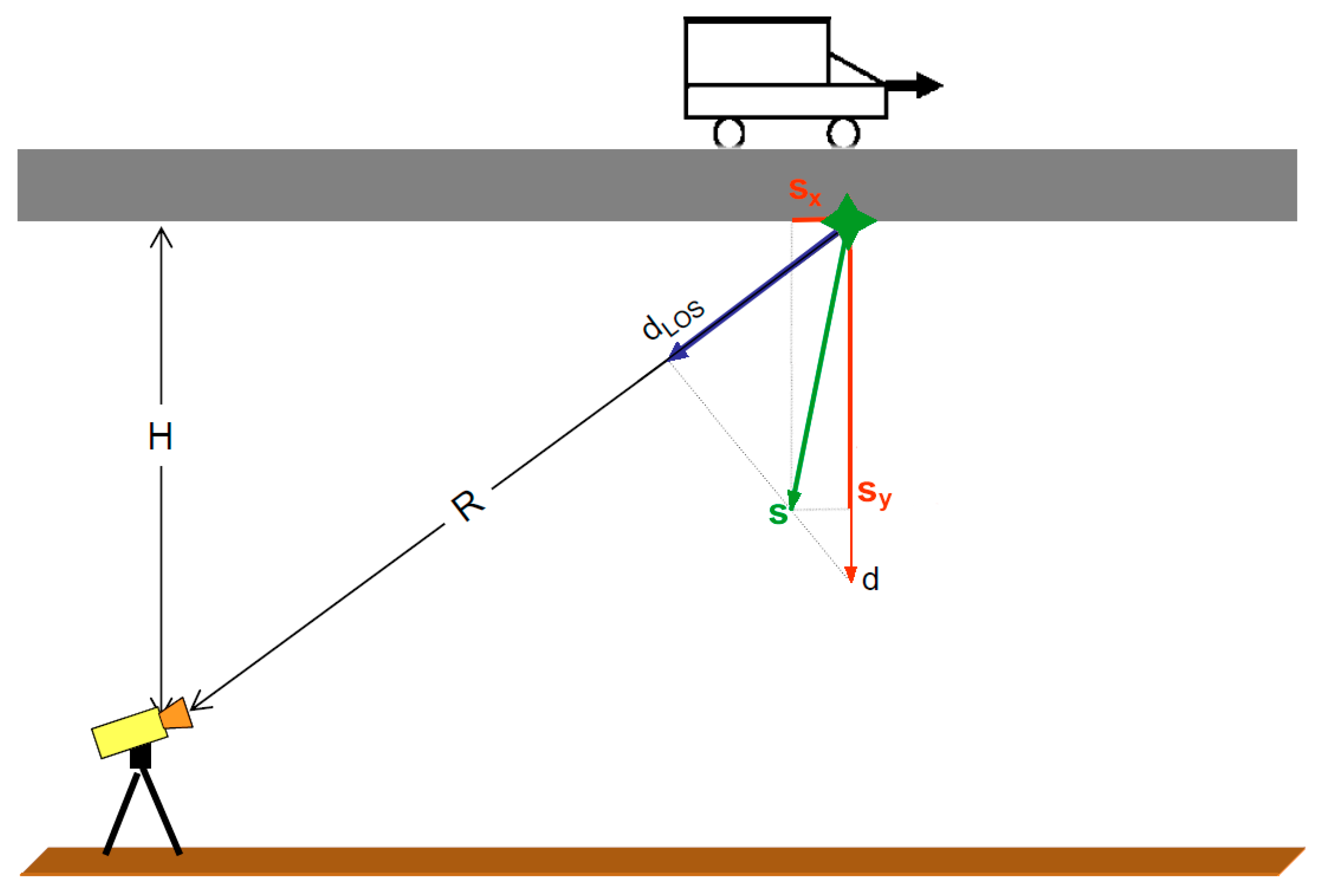
Figure 2.
Origin of the Interpretation Error EI when measuring with only one interferometric radar: s—total displacement; sy—vertical component of total displacement; sx—horizontal component of total displacement; dLOS—measured displacement in the range direction; d—calculated vertical displacement; R—radar distance from the measured point; H—radar distance from the measured point in vertical direction.
Figure 3.
Two basic configurations of the position of the two radars when measuring bridges: (a) the radars measure against each other—at the top, or (b) the radars measure from one side (radars are placed behind each other)—at the bottom.
Figure 3.
Two basic configurations of the position of the two radars when measuring bridges: (a) the radars measure against each other—at the top, or (b) the radars measure from one side (radars are placed behind each other)—at the bottom.
Figure 4.
Relationship of displacement vector to measured LOS displacements and vertical angles from radars , to the monitored point.
Figure 4.
Relationship of displacement vector to measured LOS displacements and vertical angles from radars , to the monitored point.
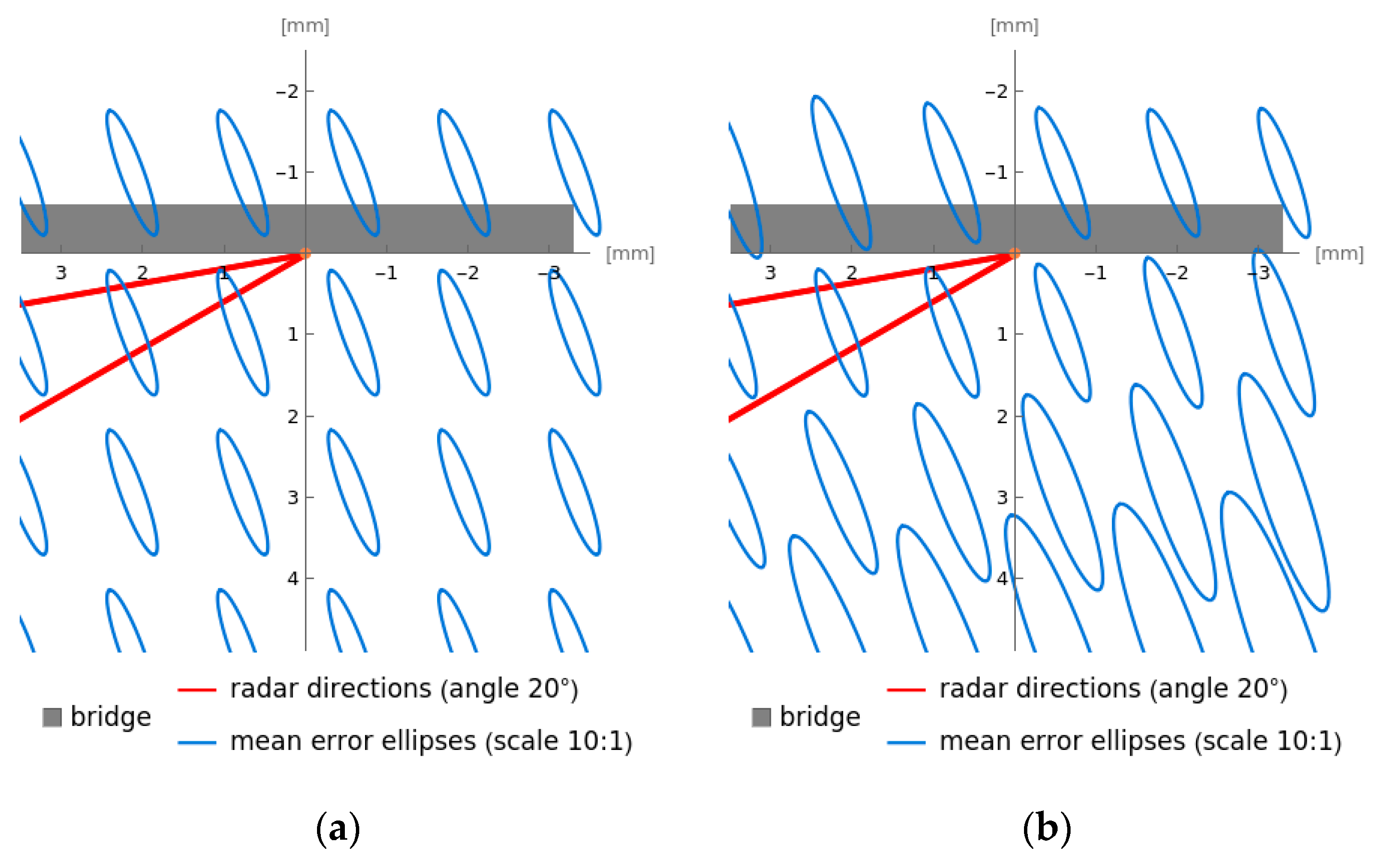
Figure 5.
Accuracy of displacement vector when the radars are located at opposite ends of the bridge and vertical angles of radar directions are and : Standard deviation of measured LOS displacements is 0.02 mm. Scale of the mean error ellipses is 10:1. (a) Imprecision of the vertical angles of radar directions was neglected; (b) precision of the vertical angles is given by means of standard deviation .
Figure 6.
Accuracy of displacement vector when radars are located behind each other, and vertical angles of radar directions are and : Standard deviation of measured LOS displacements is 0.02 mm. Scale of the mean error ellipses is 10:1. (a) Imprecision of the vertical angles of radar directions was neglected; (b) precision of the vertical angles is given by means of standard deviation .
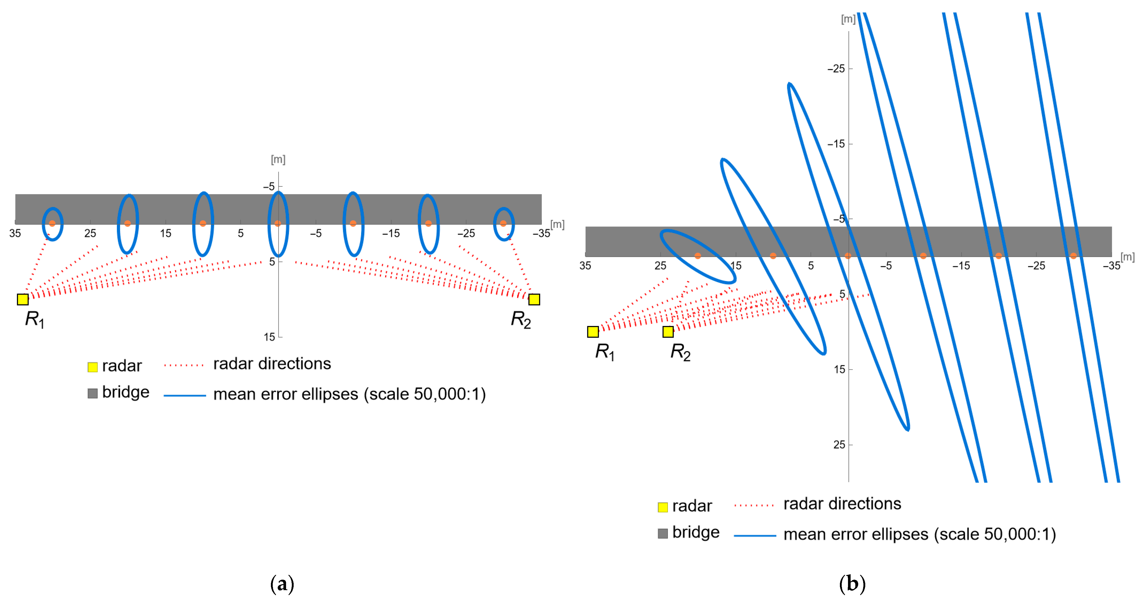
Figure 7.
Accuracy of displacement vector at various points on the bridge. Positions of the radars are determined with precision . Standard deviation of measured LOS displacements is 0.02 mm. Scale of the mean error ellipses is 50,000:1. (a) radars are placed at opposite ends of the bridge; (b) radars are placed behind each other.
Figure 8.
Standard deviations when the radars are located at opposite ends of the bridge (vertical angles of radar directions are and ). The angles are determined with precision . Standard deviation of measured LOS displacement is 0.02 mm. Numeric values on the axes and on the isolines are in mm: (a) Standard deviation ; (b) Standard deviation .
Figure 9.
Standard deviations when the radars are located behind each other (vertical angles of radar directions are and ). The angles are determined with precision . Standard deviation of measured LOS displacement is 0.02 mm. Numeric values on the axes and on the isolines are in mm: (a) Standard deviation ; (b) Standard deviation .
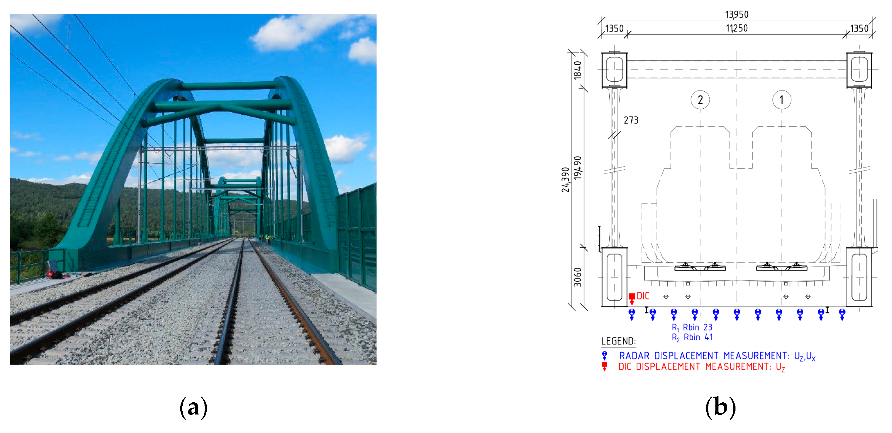
Figure 10.
Side view on the third span of the tied-arch bridge (a) photo; (b) schematic with marked positions of accelerometers and Rbins.
Figure 10.
Side view on the third span of the tied-arch bridge (a) photo; (b) schematic with marked positions of accelerometers and Rbins.
Figure 11.
The view on the load bearing structure in the third span of the bridge (a) photo; (b) schematic with marked positions of accelerometers.
Figure 11.
The view on the load bearing structure in the third span of the bridge (a) photo; (b) schematic with marked positions of accelerometers.
Figure 12.
A view of the SIRIUS data acquisition station and the left main girder with two 8344 accelerometers attached in the center of the main span of the bridge.
Figure 12.
A view of the SIRIUS data acquisition station and the left main girder with two 8344 accelerometers attached in the center of the main span of the bridge.
Figure 13.
A view of the steel crossbeams of the bridge from the position of the R2 radar (near Valy municipality). The crossbeams served as natural signal reflectors.
Figure 13.
A view of the steel crossbeams of the bridge from the position of the R2 radar (near Valy municipality). The crossbeams served as natural signal reflectors.
Figure 14.
Top view of the location of radars under the third (main) span of the bridge, values are in meters.
Figure 14.
Top view of the location of radars under the third (main) span of the bridge, values are in meters.
Figure 15.
Significant maxims on the SNR profiles of the radars (a) R1 and (b) R2.
Figure 15.
Significant maxims on the SNR profiles of the radars (a) R1 and (b) R2.
Figure 16.
Three-dimensional model of the bridge with color-highlighted Rbins for radars R1 and R2, which were evaluated.
Figure 16.
Three-dimensional model of the bridge with color-highlighted Rbins for radars R1 and R2, which were evaluated.
Figure 17.
Side view on the analyzed superstructure BS2 (a) photo; in the background there is the superstructure BS3; (b) schematic with marked positions of DIC target, Rbins, radars, and DIC camera.
Figure 17.
Side view on the analyzed superstructure BS2 (a) photo; in the background there is the superstructure BS3; (b) schematic with marked positions of DIC target, Rbins, radars, and DIC camera.
Figure 18.
View on the analyzed horizontal load-bearing structure BS2 that is oriented in the direction of its longitudinal axis (a) photo; in the background there is the superstructure BS3; (b) schematic with marked positions of DIC target, and Rbins.
Figure 18.
View on the analyzed horizontal load-bearing structure BS2 that is oriented in the direction of its longitudinal axis (a) photo; in the background there is the superstructure BS3; (b) schematic with marked positions of DIC target, and Rbins.
Figure 19.
(a) View on the test train moving across the bridge. (b) View on the accelerometer of type 8344 located on the rigid beam.
Figure 19.
(a) View on the test train moving across the bridge. (b) View on the accelerometer of type 8344 located on the rigid beam.
Figure 20.
Used interferometric radars: (a) Bottom view on the bridge deck of the structure BS2 with the steel crossbeams from the position of the radar R1; (b) View on both radars: R1 is in the foreground, and R2 is in the background in the photo.
Figure 20.
Used interferometric radars: (a) Bottom view on the bridge deck of the structure BS2 with the steel crossbeams from the position of the radar R1; (b) View on both radars: R1 is in the foreground, and R2 is in the background in the photo.
Figure 21.
Three-dimensional model of the bridge with color-highlighted Rbins for radars R1 and R2, which were evaluated, and with marked positions of both radars below the structure BS2.
Figure 21.
Three-dimensional model of the bridge with color-highlighted Rbins for radars R1 and R2, which were evaluated, and with marked positions of both radars below the structure BS2.
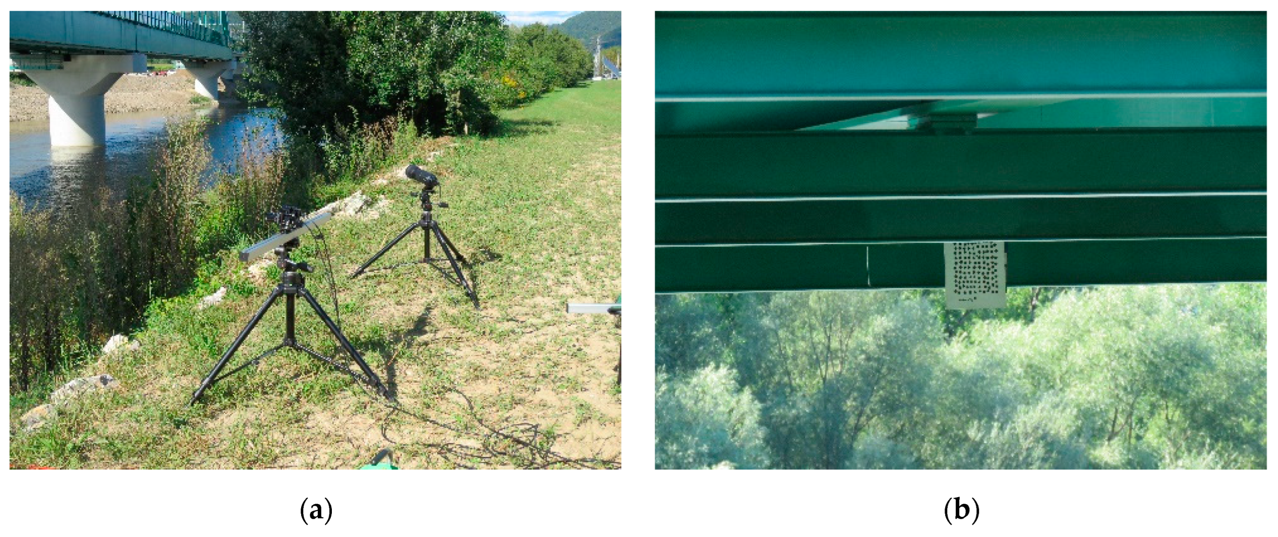
Figure 22.
Photogrammetric digital image correlation equipment: (a) Two active cameras applied during the experiment as part of the 2D-DIC system. (b) The steel boards painted by white color and by a black random pattern fixed at the observed point on the bridge deck.
Figure 22.
Photogrammetric digital image correlation equipment: (a) Two active cameras applied during the experiment as part of the 2D-DIC system. (b) The steel boards painted by white color and by a black random pattern fixed at the observed point on the bridge deck.
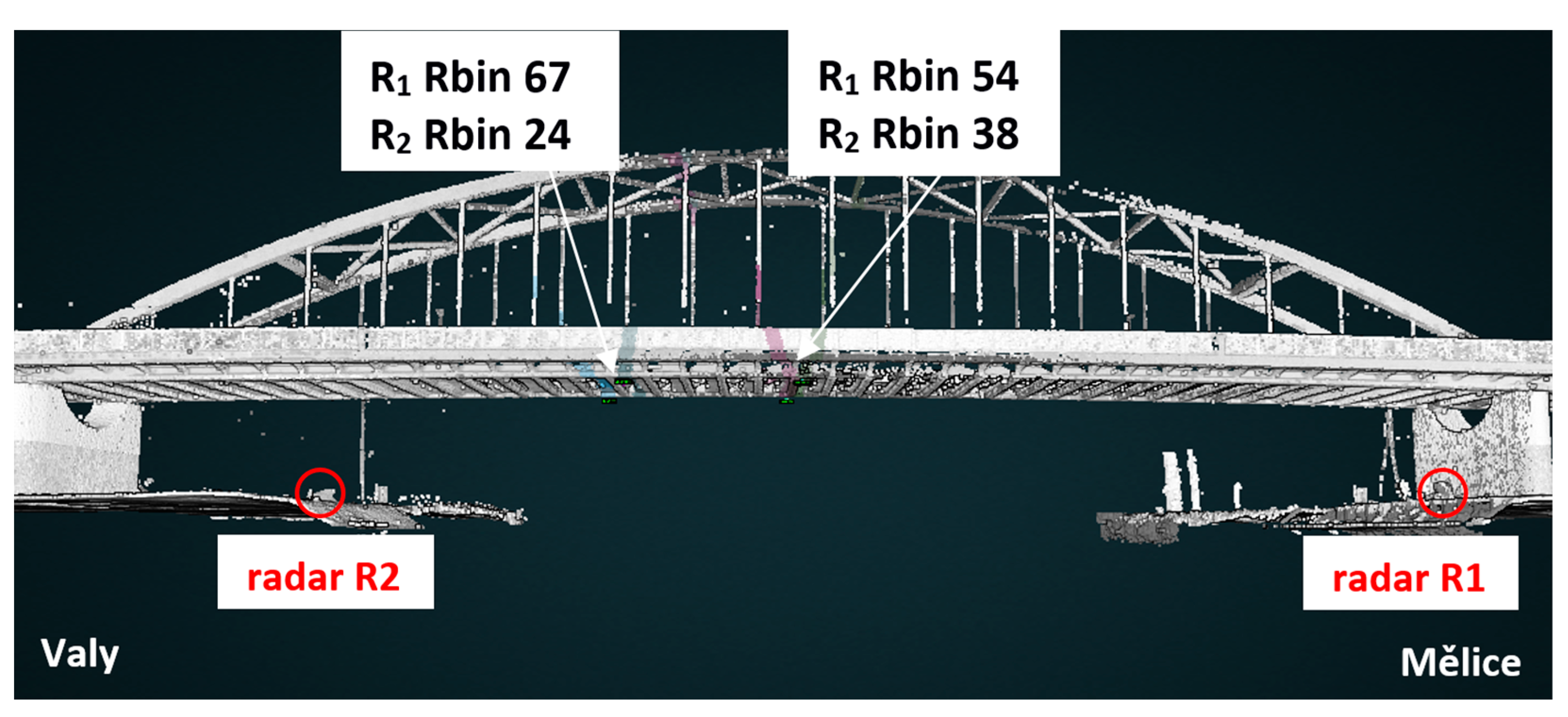
Figure 23.
Displacements, including the quasi static component demonstrated on two crossbeams (the first one corresponds to Rbins R1 54 and R2 38, and the second one to Rbins R1 67 and R2 24): at the top during the passage of the vehicle in the direction from Mělice to Valy; at the bottom caused by the regular pace of a group of pedestrians; (a,c) comparison of separately evaluated vertical displacements using Formula (1) measured by radars R1 and R2; (b,d) longitudinal and vertical displacements calculated by combination of both radar measurements (4). The Rbin numbers correspond to the R1 radar.
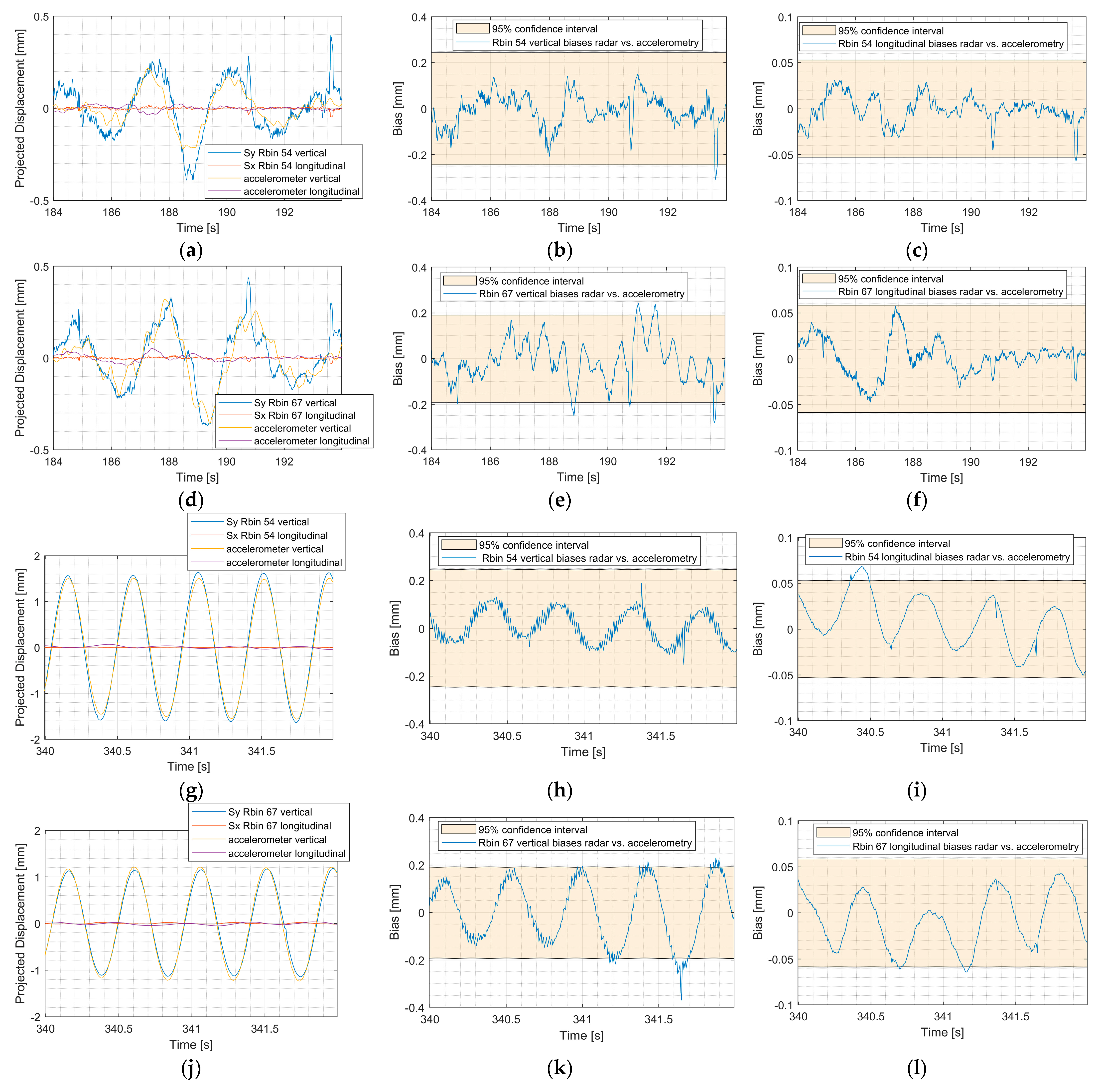
Figure 24.
Dynamic displacements evaluated using combination of both radar measurements (by Formula (4)) and corresponding displacements measured by accelerometers: 1st and 2nd row: during the passage of the vehicle in the direction from Mělice to Valy; 3rd and 4th row: caused by the regular pace of a group of pedestrians; 1st and 3rd row: for R1 Rbin 54; 2nd and 4th row: for R1 Rbin 67: 1st column (a,d,g,j): comparison of dynamic displacements with accelerometer measurements; 2nd column (b,e,h,k): comparison of vertical displacements biases between radar and accelerometer measurement with the confidence intervals. Percentage of the biases that belong into the 95% confidence interval is: (b) 99.2%, (e) 94.0%, (h) 100%, and (k) 89.5%; 3rd column (c,f,i,l): comparison of longitudinal displacements biases between radar and accelerometer measurement with the confidence intervals. Percentage of the biases that belong into the 95% confidence interval is (c) 99.4%, (f) 100%, (i) 93.5%, and (l) 97.0%.
![Remotesensing 15 00837 g024]()
Figure 25.
Comparison of total displacements biases between radar and accelerometer measurement with the confidence ellipses (15). Overlay of point clusters (black points) by 95% confidence ellipses (red curves): (a) percentage of points in the ellipse that represents accuracy of the displacement vector in R1 Rbin 54 is 98.8%; (b) for R1 Rbin 67, the percentage is 95.1%.
Figure 26.
Effect of the quasi static components on the total displacement. Longitudinal and vertical displacements caused by the regular pace of a group of pedestrians during concurrent passage of a vehicle across the bridge: (a) including the quasi static component calculated by combination of both radar measurements. The irregularity of the oscillation is caused by the vehicle crossing the bridge at the same time; (b) without the quasi static component calculated by combination of both radar measurements. (c) Corresponding longitudinal and vertical displacements converted from accelerometers measurement.
Figure 27.
Frequency spectra (periodograms)—natural, significant, and distinct frequencies of the observed bridge measured by accelerometer: 1.87, 2.23, 2.95, 3.78, 3.99, 5.52, and 7.22 Hz and by radars (Sy Rbin 54): 1.88, 2.22, 3.32, 3.74, and 3.99 Hz (a) and by accelerometer: 1.61, 1.87, 2.23, 2.46, 2.95, 3.43, 3.70, 3.99, 4.48, and 5.12 Hz and by radars (Sy Rbin67): 1.61, 1.80, 2.22, 3.42, and 3.74 Hz (b).
Figure 28.
First row: comparison of vertical displacements during the passage of the test train including 2 locomotives: (a) at 40 km/h—direction Bratislava; (b) at 50 km/h—direction Bratislava; (c) at 90 km/h—direction Žilina; second row: comparison of the confidence intervals with biases between radar and DIC measurement of vertical displacements: (d) for the train speed 40 km/h. Percentage of the biases that belong into the 95% confidence interval is 96%; (e) 50 km/h, 94%; (f) 90 km/h, 84%.
Table 1.
Values of the Interpretation Error EI for R/H and sx/sy ratios commonly used in practice.
Table 1.
Values of the Interpretation Error EI for R/H and sx/sy ratios commonly used in practice.
| R/H\sx/sy | 0.01 | 0.04 | 0.07 | 0.10 | 0.15 | 0.20 | 0.25 | 0.30 | 0.40 | 0.50 |
|---|
| 1.00 | 0% | 0% | 0% | 0% | 0% | 0% | 0% | 0% | 0% | 0% |
| 1.20 | 1% | 3% | 5% | 7% | 10% | 13% | 17% | 20% | 27% | 33% |
| 1.40 | 1% | 4% | 7% | 10% | 15% | 20% | 24% | 29% | 39% | 49% |
| 1.60 | 1% | 5% | 9% | 12% | 19% | 25% | 31% | 37% | 50% | 62% |
| 1.80 | 1% | 6% | 10% | 15% | 22% | 30% | 37% | 45% | 60% | 75% |
| 2.00 | 2% | 7% | 12% | 17% | 26% | 35% | 43% | 52% | 69% | 87% |
| 2.50 | 2% | 9% | 16% | 23% | 34% | 46% | 57% | 69% | 92% | 115% |
| 3.00 | 3% | 11% | 20% | 28% | 42% | 57% | 71% | 85% | 113% | 141% |
| 3.50 | 3% | 13% | 23% | 34% | 50% | 67% | 84% | 101% | 134% | 168% |
| 4.00 | 4% | 15% | 27% | 39% | 58% | 77% | 97% | 116% | 155% | 194% |
| 4.50 | 4% | 18% | 31% | 44% | 66% | 88% | 110% | 132% | 175% | 219% |
| 5.00 | 5% | 20% | 34% | 49% | 73% | 98% | 122% | 147% | 196% | 245% |
| 5.50 | 5% | 22% | 38% | 54% | 81% | 108% | 135% | 162% | 216% | 270% |
| 6.00 | 6% | 24% | 41% | 59% | 89% | 118% | 148% | 177% | 237% | 296% |
| 7.00 | 7% | 28% | 48% | 69% | 104% | 139% | 173% | 208% | 277% | 346% |
| 8.00 | 8% | 32% | 56% | 79% | 119% | 159% | 198% | 238% | 317% | 397% |
| 9.00 | 9% | 36% | 63% | 89% | 134% | 179% | 224% | 268% | 358% | 447% |
| 10.00 | 10% | 40% | 70% | 99% | 149% | 199% | 249% | 298% | 398% | 497% |
Table 2.
Summary of the evaluation of covariance matrix .
Table 2.
Summary of the evaluation of covariance matrix .
| Case | | Substitutions |
|---|
| LOS imprecision neglected | | (14), (13) |
| LOS precision considered | | (12), (10), (16), (13), (17) |
Table 3.
Settings of used radars (bridge Valy).
Table 3.
Settings of used radars (bridge Valy).
| | R1: Radar IBIS—FS Plus | R2: Radar IBIS—RU 172 |
|---|
| Sampling frequency | 200 Hz | 199.2 Hz 1 |
| Signal range (max. distance) | 75 m | 70 m |
| Rbin (range resolution area) | 0.75 m | 0.75 m |
Table 4.
Settings of used radars (bridge Púchov).
Table 4.
Settings of used radars (bridge Púchov).
| | R1: Radar IBIS—FS Plus | R2: Radar IBIS—RU 172 |
|---|
| Sampling frequency | 200 Hz | 199.2 Hz 1 |
| Signal range (max. distance) | 100 m | 120 m |
| Rbin (range resolution area) | 0.75 m | 0.75 m |
| Vertical tilt of the radar | 0.0° | 53.9° 1 |


 ,
, 


