Mapping the Groundwater Level and Soil Moisture of a Montane Peat Bog Using UAV Monitoring and Machine Learning

Abstract

One of the best preconditions for the sufficient monitoring of peat bog ecosystems is the collection, processing, and analysis of unique spatial data to understand peat bog dynamics. Over two seasons, we sampled groundwater level (GWL) and soil moisture (SM) ground truth data at two diverse locations at the Rokytka Peat bog within the Sumava Mountains, Czechia. These data served as reference data and were modeled with a suite of potential variables derived from digital surface models (DSMs) and RGB, multispectral, and thermal orthoimages reflecting topomorphometry, vegetation, and surface temperature information generated from drone mapping. We used 34 predictors to feed the random forest (RF) algorithm. The predictor selection, hyperparameter tuning, and performance assessment were performed with the target-oriented leave-location-out (LLO) spatial cross-validation (CV) strategy combined with forward feature selection (FFS) to avoid overfitting and to predict on unknown locations. The spatial CV performance statistics showed low (R² = 0.12) to high (R² = 0.78) model predictions. The predictor importance was used for model interpretation, where temperature had strong impact on GWL and SM, and we found significant contributions of other predictors, such as Normalized Difference Vegetation Index (NDVI), Normalized Difference Index (NDI), Enhanced Red-Green-Blue Vegetation Index (ERGBVE), Shape Index (SHP), Green Leaf Index (GLI), Brightness Index (BI), Coloration Index (CI), Redness Index (RI), Primary Colours Hue Index (HI), Overall Hue Index (HUE), SAGA Wetness Index (TWI), Plan Curvature (PlnCurv), Topographic Position Index (TPI), and Vector Ruggedness Measure (VRM). Additionally, we estimated the area of applicability (AOA) by presenting maps where the prediction model yielded high-quality results and where predictions were highly uncertain because machine learning (ML) models make predictions far beyond sampling locations without sampling data with no knowledge about these environments. The AOA method is well suited and unique for planning and decision-making about the best sampling strategy, most notably with limited data.

1. Introduction

On a global scale, peatlands as a group of wetlands are essential for the landscape and environment because they provide a wide range of critical ecosystem services [1], water-quality improvement, flood abatement, and habitat functions. However, peatlands are decreasing globally in terms of their condition and diversity through habitat loss, climate change, and pollution [2]. Peat bogs, a subdivision of peatlands, in particular, are significant water-logged reservoirs with a specific hydrological regime [3], representing habitats dominated by sphagnum moss, stored organic matter, a high water table, and low pH [4,5]. The Sumava Mountains (Sumava Mts., Bohemian Forest) feature the most extensive peat bog complex in Central Europe due to their specific geology and morphology [6]. Similar upland peat bogs occur in Canada, Scotland, and Scandinavia. However, Sumava’s mountainous peat bog complexes have a specific regime concerning a humid climate and optimal relief configuration [6] to study specific dynamics over time. Various human activities have affected the peatlands in the Sumava Mts. in past decades [7]. Among these human activities, artificial surface drainage is one of the most critical threats [8], affecting approximately about 70% of the peat bogs in Sumava National Park (Sumava NP).

To understand the hydrological regime and the effects of human impacts on the peatlands in Sumava NP, extensive research on hydrology [6,9,10,11,12,13,14,15], vegetation [16], soil [14], restoration of mires [8,15], and soil water dynamics [17] have been conducted. All these studies required invasive fieldwork or analysis, requiring demanding and recurrent field monitoring and surveying campaigns. Peatland complexes represent the zone with the highest status of nature protection with restricted access and limited invasive surveying and monitoring activities. For such specific environments, there is the emerging importance of novel monitoring approaches that minimize the impact on protected areas.

Recent advances in drones (a.k.a., unmanned aircraft systems, UASs, unmanned aerial vehicles, UAVs, or remotely piloted aircraft systems, RPAS) and the miniaturization of advanced sensors present new potential for noninvasive methods to monitor natural processes, even in inaccessible or sensitive areas. Due to sensor miniaturization, it is now possible to choose between different camera systems spanning from heavyweight LiDAR (light detection and ranging) to lightweight RGB, multispectral, and thermal mapping sensors [18], enabling unforeseen future research fields. These abilities make drones particularly attractive for ultrahigh-resolution imagery and 3D point clouds, independent of weather and cloud coverage to capture small-scale variabilities of the land surface in high detail. Recent improvements in drone technology have provided exciting new abilities for peatland observation, providing a noninvasive alternative to conventional fieldwork. Earlier, these skills allowed the investigation of a high-resolution classification of South Patagonian peat bogs and showed potential gaps in upscaled CH4 fluxes using UAV system color-infrared (CIR) imagery [19]. Additionally, [20] examined Alberta’s water table dynamics in Canada using drones and demonstrated the potential for measuring over large areas using UAV technology, thus providing insights into the impacts of disturbances on hydrology and related ecosystem functions. [21] used UAV remote sensing to map water depth over large areas to show methane release in a treed bog ecosystem in northern Alberta, Canada. A year later, [22] studied seismic lines generated by CH4 flux estimates based on microtopography and depth to water features using photogrammetric inputs. Additionally, [23] used thermal imagery equipped on a UAV to identify groundwater discharges and the usefulness of thermal validation concerning process-based restoration goals in Massachusetts, USA.

Further, [24] used UAV-based thermal infrared (TIR) imaging and color infrared imaging, combining stable water isotope studies to identify treatments along a mining area in Finland. Most studies practiced one or two sensors in studying peatland environments. To overcome these issues, [25] used multiple sensor records with a fixed-wing UAV at two rewetted fen sites in northern Germany (Mecklenburg Western Pomerania) and classified spectrally similar vegetation. That study made satisfactory predictions of vegetation types based on two multitemporal and multi-sensor datasets, via machine learning (ML).

Frequently, predictive modeling using ML has been used to show spatial and spatiotemporal patterns and changes in the environment [26,27,28,29,30]. Additionally, predictive modeling is commonly used with field data to train demographic models with spatial continuous predictor variables obtained from remote sensing images [28,30]. Those models can typically make predictions for an entire area of interest [30], even exceeding training data locations without knowing about these environments, which is one of the drawbacks of conventional ML methods, such as random forest (RF) [31]. Moreover, ML has been criticized for overfitting [30,32]; for example, complex models with many parameters can obtain both global trends and noise-generated intentions simultaneously. In this case, the model can be outwitted into thinking that the noise encodes real information. This overfitting yields a steep decrease in predictive performance [32]. To guard against vague predictions beyond sampling locations and overfitting, [33] proposed an improved model that yielded better performance. Therefore, we took advantage of their ML prediction strategy using forward feature selection (FFS) for optimal variable selection in conjunction with the leave-location-out (LLO) cross-validation (CV) method to: (1) reduce the overfitting of noisy variables; (2) not estimate model performances based on the random k-fold CV but rather apply this target-oriented validation strategy in the context of unknown space; and (3) estimate the area of applicability (AOA) to find the area where prediction is positively specific or uncertain using the dissimilarity index (DI) [33].

Our research aimed to obtain information and predict the dynamic properties of groundwater level (GWL) and top-layer soil moisture (SM) in 2 dimensions and time (2D + T) based on data from digital surface models (DSMs), RGB, multispectral, and thermal data from drone imagery. We used a CAST spatiotemporal prediction model based on an RF algorithm and the FFS method in conjunction with target oriented LLO CV validation [32]. Compared to other models, the CAST model yields the advantage of dismissing unsuitable predictors and estimating the AOA automatically.

The specific objectives of this study were to:

• Collect UAV RGB, multispectral, and thermal imagery along with ground truth data on GWL and SM over ten months;
• Extract a suite of variables (microtopographic drivers, vegetational, and temperature information) using a multi-sensor (RGB, multispectral, and thermal sensors) UAV monitoring approach;
• Spatiotemporally predict GWL and SM by the CAST ML model and assessing the importance of selected drivers; and
• Simulate prediction certainties across study areas, mimicking the environmental reality.

2. Materials and Methods

2.1. Site Description and Climate

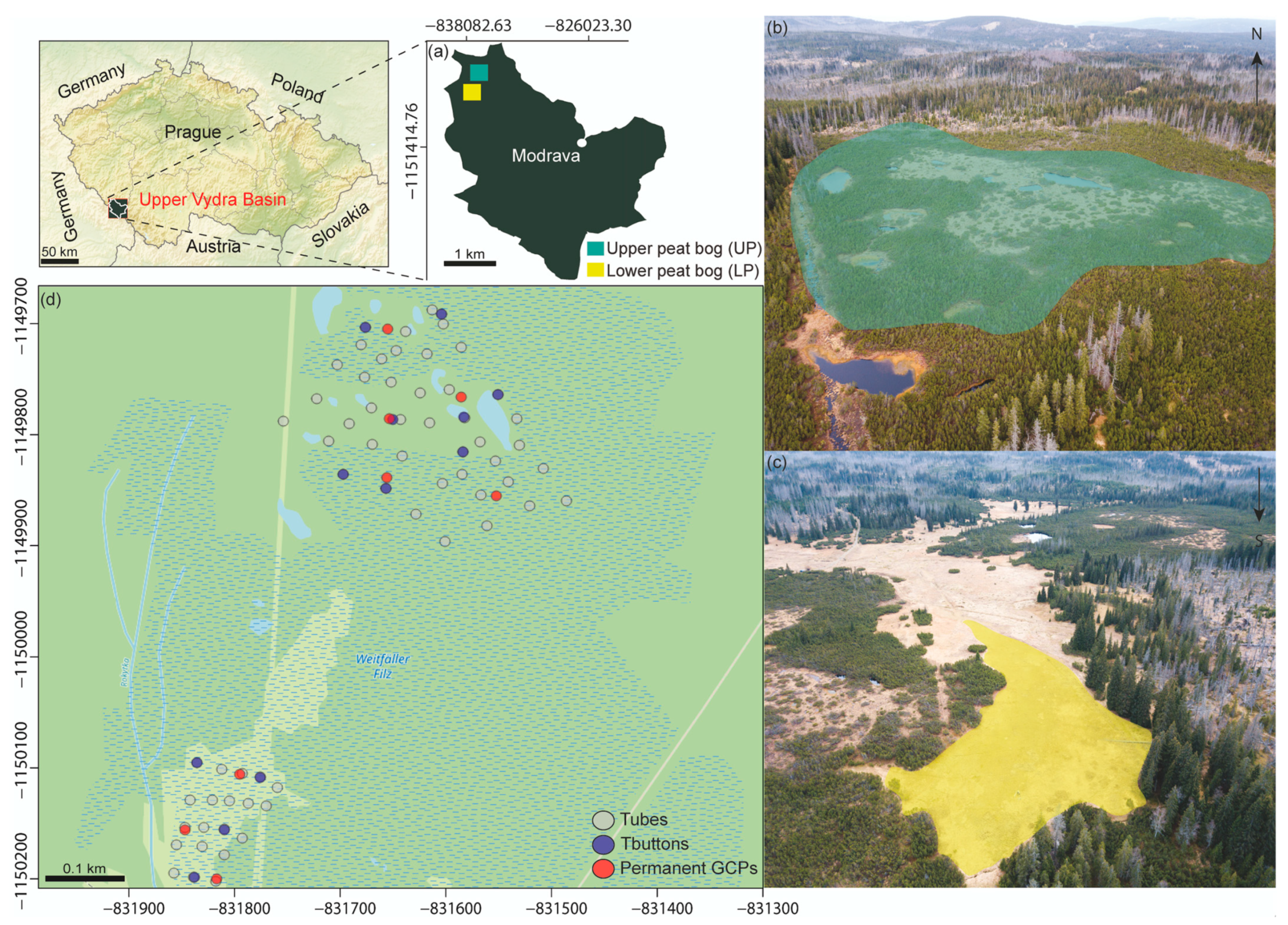
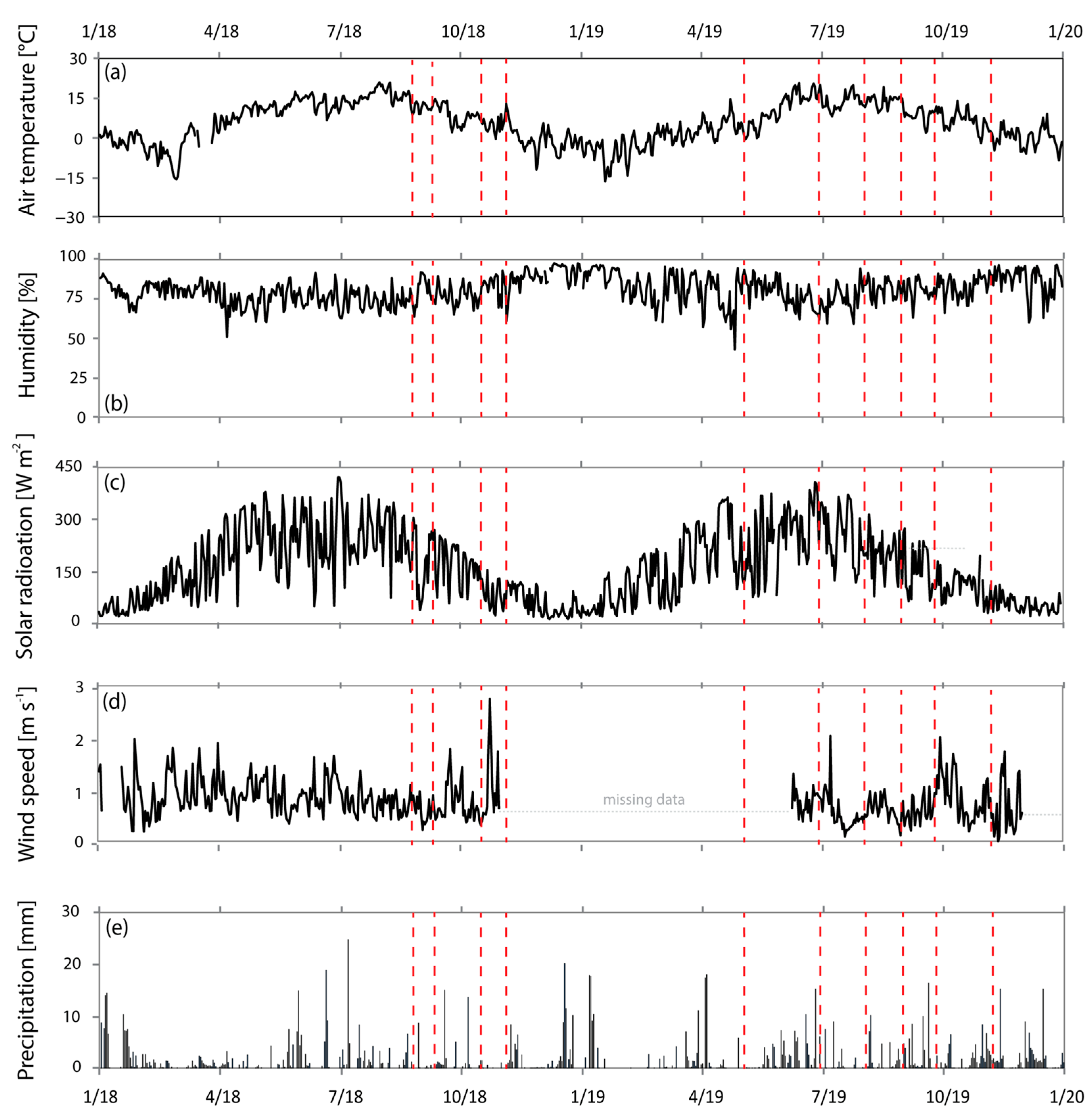
We conducted our study in the Rokytka Peat bog, one of the most extensive montane raised ombrotrophic peat bog complexes (250 ha) within the Sumava Mts., Czechia. We selected one of four large bog sites located along the Rokytka stream, a second-order stream of a river that drains an area of 0.6 sq. km with an altitude range between 1100 and 1260 m a.s.l. [12], at two test sites (Figure 1). The Upper Part test site (UP, S-JTSK/Krovak East North coordinates: −830762.40, −1149825.37, ~4.5 ha) is an open treeless site with several pools and a complex system of hummocks and hollows with flat areas in between, mostly covered by pine (Pinus mungo Turra), blueberry (Vaccinium myrtillus L.), and moss (Sphagnum sp.) vegetation (Figure 1b). The Lower Part test site (LP, S-JTSK/Krovak East North coordinates: −831134.77, −1150331.52, ~1,5 ha) is a flat zone consisting mainly of moss and cotton grass (Eriophorum sp.) (Figure 1c). Both sites are surrounded by dead spruce with healthy seedlings in the lower part and various dwarf communities. The climate in this area is variable and subject to both oceanic and continental influences. Due to the specific morphology and peat bog open space area, the Rokytka catchment is one of the coldest places throughout the country in January or February (Figure 2). Freezing temperatures can occur even during summer, and the average daily air temperature is 4.8 °C (Figure 2a). This locality also belongs to one of the Czech Republic’s wettest parts. Humidity varies more during the day than during a year (Figure 2b), and solar radiation shows regular annual behavior with highs in summer and lows in winter (Figure 2c).

All meteorological parameters except precipitation are measured in the experimental catchment with Fiedler devices without an external heating system during winter (Figure 3a). Therefore, several wind speed data gaps occurred when a wind propeller freezes (Figure 2d). Precipitation measured at nearby the Filipova Hut meteorological station at a similar altitude equaled 1239 mm yr⁻¹ (1981–2010) [34]. However, the last two years were dryer compared to the long-term average, with an annual precipitation of 1093 mm yr⁻¹ (Figure 2e).

The experimental site contains a well-developed raised ombrogenous peat bog with the dominant soil type being Histosol with a depth varying from 0.5 m (LP) to approximately 6 m (UP).

Organic matter in the soil is heterogeneous and can be found in different stages of decomposition that vary throughout the peat bog. The storm hydrograph at the catchments (0.65 sq. km) where the experimental peat bog is located is highly variable, with quickly and steeply rising and falling limbs. The hydrological response to rainfall events was fast, and the recession to antecedent base flow occurred rather quickly (Figure 2e). The mean daily runoff equaled 3.4 mm per day (1297 mm y⁻¹) at the outlet.

The UP is drained naturally into the local stream, and the vegetation of peat bogs varies based on the water regime. Grass parts without trees where this experiment occurred belong to areas where the groundwater table occurs near the surface. Soil is primarily saturated with water during the year. The LP hydrological response is probably affected by one drainage ditch. However, due to the high hydraulic conductivity of peat, the channel drains only a small buffer [15]. In general, UP and LP did not differ in SM or GWL, which can be proven by their similar vegetation cover (grass, moss).

2.2. Ground Survey

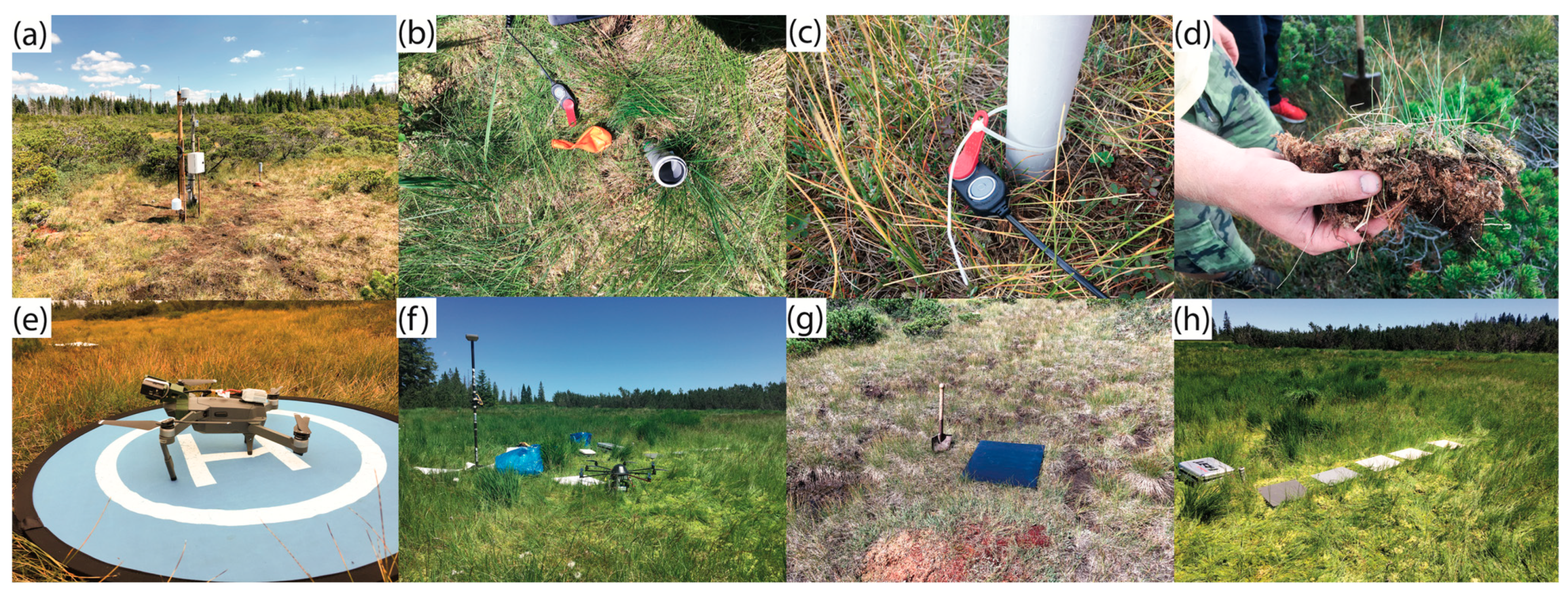
Field surveys and airborne campaigns occurred between August and November 2018, and between May and November 2019 for a total of 10 days of data collection (Figure 2; represented by red dashed lines). For the GWL measurements, we installed 63 water tubes around the study area, 43 at the UP (Figure 1d), and 20 at the LP (Figure 1d). For the wells, we employed 1 m long and 2.5 cm diameter PVC pipes (Figure 3b) perforated through nearly their entire length to allow water to infiltrate, and we manually installed them into soft peat soil. We measured the GWL within the wells in Figure 3h for each UAV survey using a blowpipe and a scale. We used the blowpipe to identify the tube’s water level and a measuring tape to record the water ground-level depth, similar to [14]. Additionally, we collected 63 samples of the topsoil next to the wells (Figure 3d) at both sites, which were dried in the laboratory to obtain the gravimetric soil water content (GWC) of the surface peat material taken from the samples to determine moisture content. GWC is the mass of water per mass of dry soil in a given sample. The taken soil probe was first weighed and then dried in an oven at 105 °C for at least three days, depending on the soil material. The equation for GWC (θg) is:

θg = (Wet − Dry)/Dry

(1)

where Wet is the weight of the soil sample from the field and Dry is the weight of the dry soil sample. Further, we installed 12 Thermochron iButton (model DS1921G-F5#) loggers (hereafter referred to as Tbuttons, Figure 3c), 8 in the UP and four in the LP, to validate the topsoil surface temperature estimates during thermal imagery. In situ ground truthing is required for UAV thermography radiometric calibration due to spatiotemporal variations in air temperature, humidity, and atmospheric aerosol concentrations [34]. The Tbuttons logged the temperature at half-hour intervals with an accuracy of ±1 °C, sampling 2048 temperature readings that allowed thermal imagery calibration later (Section 2.4). We measured the exact position of the Tbuttons and wells with a Topcon HiPer SR geodetic global navigation satellite system (GNSS) receiver with a horizontal accuracy of 1.8 cm and a vertical accuracy of 2.5 cm using a real-time kinematic method with a virtual reference station.

2.3. UAV Platforms and Cameras

UAV campaigns were conducted with ground surveys. We used two different UAV platforms. For the first flight, a commercial Mavic Pro (DJI Co.) drone was used to acquire nadir-viewing aerial imagery of the peat bog surface. We attached a second gimbal (MAPIR Survey3 Mount) with a FLIR DUO R dual-sensor RGB/thermal camera on the drone to capture thermal band (IR) imagery in the spectrum from 750 to 1350 nm set to an interval of 1 sec (Figure 3e). The mount was at a fixed 17-degree tilt that oriented the camera nadir during the maximum forward surveying flight speeds of approximately 8 m/s (https://www.mapir.camera/products/dji-mavic-pro-mapir-survey-3-single-camera-mount, accessed on 23 March 2020). The thermal data were saved in Radiometric JPEG format to preserve the temperature values for every pixel. The resolution of the thermal lens is comparatively low (160 by 1220 pixels). The FLIR camera did not have a GPS sensor; thus, we distributed black 0.5 m × 0.5 m targets as ground control points (GCPs) (Figure 3g). For the second flight, we equipped the second drone, a MikroKopter ARF XL, with a miniaturized camera (Tetracam μ-MCA Snap 6) to acquire near-infrared (NIR) images of 550 to 900 nm every second in continuous mode (Figure 3f). We positioned five validation targets with known reflectances in the field (Figure 3h). We used, white 0.5 m × 0.5 m targets as GCPs for the multispectral overflights (Figure 3f) and conducted RGB and thermal overflights at a height of 60 m to ensure visibility of the surface cover and the black targets visibility in the thermal images. The multispectral overflights were taken at a height of 80 m due to the narrow shooting angles of the Tetracam. We measured the GCPs with the GNSS receiver Topcon (Section 2.2). Five permanent GCPs at the UP and three permanent GCPs at the LP with additional temporary distributed GCPs each time during the field campaign served as co-registration of all scenes taken by the different sensors (Figure 1d). All specifications of drones and sensors are shown in Table S1.

2.4. Data Processing

2.4.1. RGB Scenes

The two test sites (UP and LP) were flown across ten times over with nearly every sensor (

Table 1. Peat bog data set spatiotemporal predictors and ground truth responsive variables.

Predictor Variables	Definition	Formula
RGB spectral indices (orthoimages)
RGI	Red-green ratio index [40]	(red/green)
VVI	Visible vegetation index [41]	(1 − (red − 30)/(red + 30)) * (1 − (green − 50)/(green + 50)) * (1 − (blue − 1)/(blue + 1))
VDVI	Visible-band Difference Vegetation Index	(2 * green − red − blue)/(2 * green + red + blue)
VARI	Visible Atmospherically Resistant Index	(green-red)/(green + red-blue)
TGI	Triangular Greenness Index [42]	−0.5[190(red670 − red550) − 120(red670 − red480)]
SI	Spectral Slope Saturation Index	(red-blue)/(red + blue)
SHP	Shape index	2 * (red − green − blue)/(green − blue)
SCI	Soil Colour Index	(red-green)/(red + green)
SAT	Overall Saturation Index	max(red, green, blue) − min(red, green, blue))/max(red, green, blue)
NGRDI	Normalized Green Red Difference Index [43]	(green-red)/(green + (red))
NDTI	Normalized Difference Turbidity Index Water [44]	(red-green)/(red + green)
NDI	Normalized Difference Index	(red-green)/(red + green)
HI	Primary Colours Hue Index [45]	(2 * red-green-blue)/(green-blue)
GRVI	Green-Red Vegetation Index	(green-red)/(green + red)
GLI	Green Leaf Index [46]	(2 * green − red − blue)/(2*green + red + blue)
GLAI	Green Leaf Area Index	(25 * (green − red)/(green + red − blue) + 1.25)
ExG	Excess Green	2 * green-red-blue/red + green + blue
ERGBVE	Enhanced Red-Green-Blue Vegetation Index	3.14159 * ((green2-(red * blue))/(green2+(red * blue)))
CI	Coloration Index	(red − blue)/red
BI	Brightness Index	sqrt((red2 + green2 + blue*2)/3
RI	Redness Index	red2/(blue*green3)
HUE	Hue Overall Index	atan(2 * (red − green − blue)/30.5 * (green − blue))
Vegetation index (Multispectral scenes)
NDVI	Normalized Difference Vegetation Index [43]	(NIR-red/NIR + red)
Topomorphometric indices (DSMs)
Slope	Steepest Slope Angle [°]
ProfCurv	Profile Curvature [°]	Direction of the steepest slope. Affects the acceleration or deceleration of water [47].
PlnCurv	Plan Curvature [°]	Horizontal curvature intersecting with the x–y surface plane. Affects the convergence or divergence of water [47].
WEI	Wind Exposition Index	Values below 1 indicate wind-shaded areas, whereas values above 1 indicate areas exposed to the wind.
TRI (1, 4)*	Terrain Ruggedness Index (1)* [m]	A measure of terrain complexity/heterogeneity. It calculates the sum change in elevation between a grid cell and its neighboring grid cells. The moving window radius determines how many cells are used to calculate the elevation change [48]. Value is always ≥ 0 m, where 0 represents the minimum roughness.
VRM (1, 4)*	Vector Ruggedness Measure	A measure of terrain complexity/variance that captures variability in slope and aspect in a single measure. Ruggedness is measured as the dispersion of vectors orthogonal to the surface within a specific neighborhood. The radius of the moving window determines how many cells are used to calculate the change in ruggedness.
TPI	Topographic Position Index	Difference between the elevation of the cell and the mean of the elevation in surrounding cells [49]. Value is positive when the point is higher than its surroundings, zero when in a flat area or mid-slope, and negative when lower than its surroundings.
TWI	SAGA Wetness Index [37]	Describes the tendency of an area to accumulate water.
Thermal information (Thermal scenes)
Temperature	Relative Surface Temperature [°C]
Ground truth observation variables
GWL	Groundwater Level [cm]	Describes the source of soil water as well precipitation in peatland ecosystems.
SM	Gravimetric Water Content	Controls soil respiration that is defined as a sum of organic matter decomposition and root respiration.

* Topomorphometric variables calculated using variable radii. The lower radius indicates the immediate location conditions, whereas the higher radius indicates broader microtopographic microclimate conditions.

). Most flights were performed around solar noon or in the early afternoon and under stable cloud cover (no clouds or sparse cloud cover). We processed all data (RGB, multispectral, and thermal images) in Agisoft Metashape Professional 1.6.2 (https://www.agisoft.com, accessed on 19 January 2021) high accuracy settings and only generic preselection. RGB dense clouds were generated using high settings and aggressive depth filtering and then converted to orthomosaics (3 cm/pixel) based on the DSMs. Point clouds were georeferenced to the EPSG:5514 coordinate system (S JTSK/Krovak East North) using permanent GCPs (Figure 1d) to evaluate alignment accuracy. Black targets that were visible by both the RGB and thermal sensors were positioned on the permanent markers (Figure 3g). The GCPs were manually marked in three to four images for each GCP until the algorithm picked up their correct locations across all images. This referencing also optimized the sparse point cloud, thereby mitigating distortion effects [35]. The resulting RGB orthomosaics were then used to calculate a suite of 22 vegetation spectral index maps using the uavRst v0.5-4 [36] remote sensing toolbox in R (Table 1). We derived the topomorphometric features listed in Table 1 using the SAGA GIS modules in QGIS [37].

2.4.2. Multispectral Scenes

Before loading the multispectral imagery into Agisoft, we performed radiometric corrections (noise and vignetting reductions) following [38], using appropriate values taken under controlled laboratory conditions. Band 4 was set as a master channel for processing in Agisoft. We used very-high settings and aggressive depth filtering for multispectral dense cloud generation. Before converting the imagery to orthomosaics (0.03 m/pixel), we performed radiometric calibration using the values from the five reflectance targets based on laboratory values and the empirical line method (Section 2.3, Figure 3h) according to the method of [38]. This method yields better results than the rapid-based calibration correction of images taken during the field campaign, as stated in [39]. In this study, white targets were used for georeferencing the multispectral scenes (Figure 3f). From the multispectral orthomosaics, the normalized difference vegetation index (NDVI) was calculated using the raster calculator in Metashape.

2.4.3. Thermal Scenes

We saved the thermal data as radiometric JPGs and then converted them to 16-bit tiffs, which are favorable for processing in Agisoft. Additionally, we used very high settings and aggressive depth filtering for thermal dense cloud generation. Georeferencing was performed using black GCP targets for the RGB scenes. From DSMs, thermal orthomosaics were created to show a thermal signature in DN values ranging from 0 to 65535. Usually, DN values can be converted to temperatures on the principle of the Stefan–Boltzmann Law [50] as pixel DN values of the thermal band are proportional to the flux of infrared radiation received by the thermal lens [51]. A simple solution is to apply the calibration method reported in [51], the so-called pixel-by-pixel analysis, where all DN values in the thermal band are converted to near-real temperatures. In this study, we used only Tbuttons during the flights to measure ground objects temperature (Section 2.2, Figure 3c). In some cases, the flights took longer than half an hour; thus, we used the mean value measured by the Tbuttons. Concerning the thermal orthomosaics, we created a point shapefile with Tbutton localities with a 1 m buffer centered on the object used to extract the mean DN of the ground object. We performed linear regression between the sampled temperatures and the corresponding DNs [52]. The regression equation was then used to convert the thermal orthomosaics to the relative temperature maps that were used in the raster calculator in Metashape.

2.4.4. Input Variables

This study’s final training dataset consists of GWL measurements from installing tubes one meter deep at 63 locations distributed over two locations, where data was recorded one day during each of ten months (10 days, Table 1). We also sampled the top-surface soil moisture at the same 63 locations next to the tubes but only for seven months (7 days, Table 1); three months are missing because the peat bog’s soil moisture does not change much during the autumn months and was skipped.

A suite of several auxiliary potential predictor variables was used in this study to predict GWL and SM. Several spatially continuous variables that describe the terrain and can be geometrically characterized by DSMs and many other predictor variables were defined as spatially constant but vary in time as temporal predictor variables. These variables are represented by index maps from orthoimages. Orthoimages are prone to creating many different ratio maps depending on the camera system. Thus, we used a suite of potential vegetation indices based on the RGB scenes as spatial and temporal indicators of GWL and SM (Table 1). Therefore, vegetation is responsive to water regime (i.e., dry surfaces cause changes in the surface temperature), and we also extracted the relative surface temperature from thermal scenes. TIR imaging is also used to estimate the temperature of various surfaces, which allows mapping of temperature patterns providing information on hydrological processes [24].

Additionally, the calculated NDVI data from multispectral orthoimages deliver valuable information with regard to land surface characteristics [53] and represent a key challenge for understanding ecosystem respondents’ climate change [54]. Table 1 shows the full list of predictors used in this study. The spatial resolution layer outputs from all predictors were obtained at 0.03 m.

2.5. Model Description

Figure 4 shows a simplified flow chart of the methodological approach. After creating all index maps for each month, we stacked each month’s layers to gather information on environmental variables in space and time at the UP and LP based on limited field data for that day within a given month. We cropped all layer stacks to a smaller extent, and certain layer stacks contained 32, 33, or 34 layers (maximum number of rasters) due to missing data (see Section 2.4.4). In R, we used an automated data value extraction script based on a point shapefile (63 tube locations) to derive all values from each predictor variable for the training samples (Figure 4). Each training sample contained extracted information from all potential predictor variables (Table 1) and the GWL and SM information as much as possible based on the reference points. Before making predictions, we eliminated highly linear correlated predictors with absolute correlations above 0.75, zero- and near-zero variance variables [55], and thus raster layers containing incomplete data to reduce redundant data due to correlation, NANs, and near-zero (Figure 4) [32,56]. With this step, we did the first preselection of our input variables without losing information; however, we reduced the training time significantly during the model performance. Ideally, descriptors should be uncorrelated, as an abundant number of correlated features can hinder the model’s efficiency and accuracy. When this phenomenon occurs, different feature selection is necessary to mitigate issues with dimensionality, simplify models, and improve their interpretability and training efficiency [31]. Many other statistics can be used for variable selection, e.g., T-test, F-test, or Mallows CP, whereby different criteria may lead to very different preselection of variables [57]. Most analysis is based on the CAST [33] and caret packages [58] in R (R Core Team, 2020), which provide a wrapper to the RF algorithm [31], implementing functionality for data splitting and CV (Figure 4). Caret is needed for model training. CAST supports the caret package to provide an accounting for spatiotemporal dependencies during prediction, and CAST includes the “FFS” function for optimal variable selection and the major functionality of the “aoa” function that is doing the distance-based estimation of the AOA as we aimed to model GWL and SM far beyond the data loggers to determine how well the model performs (Figure 4).

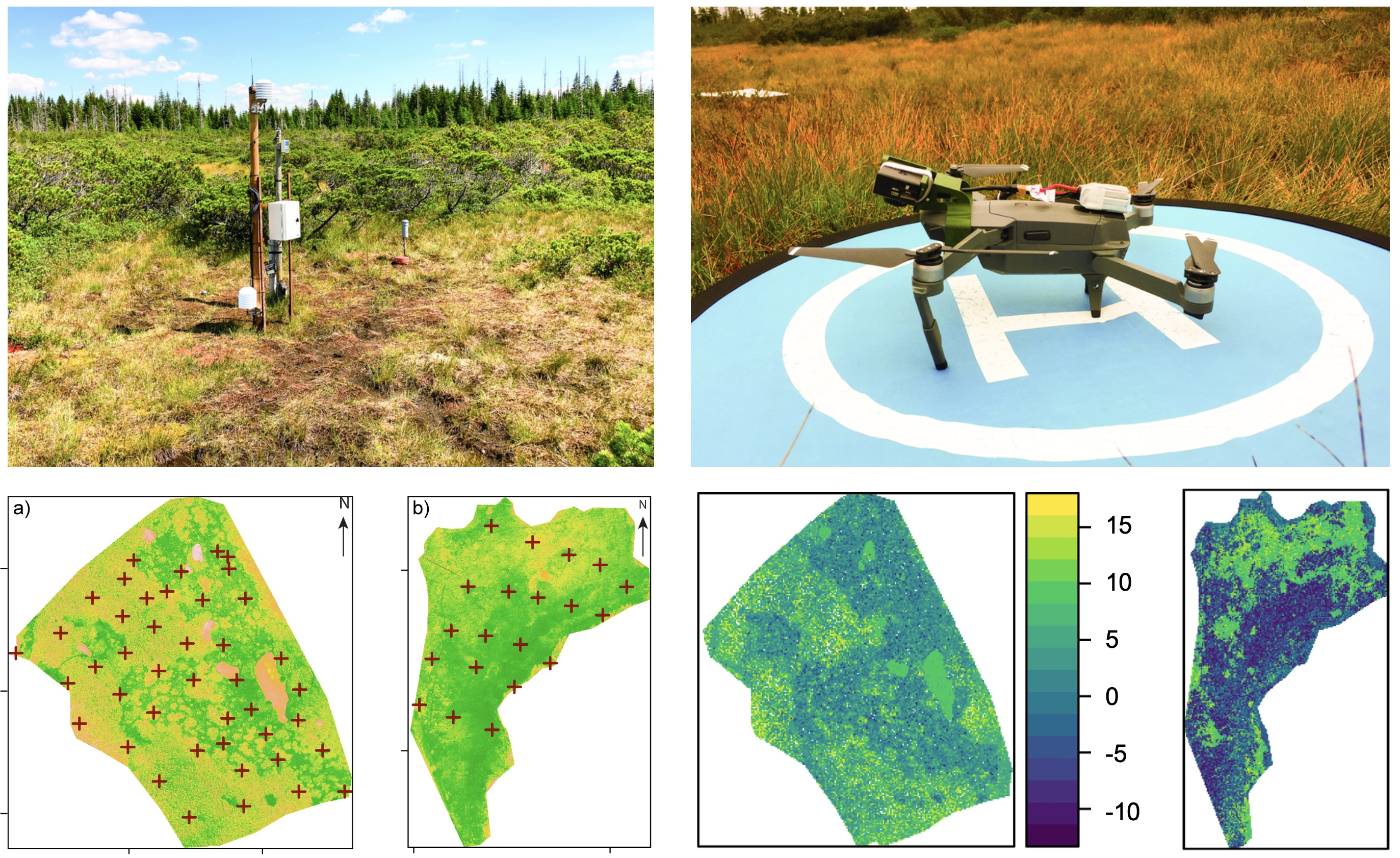
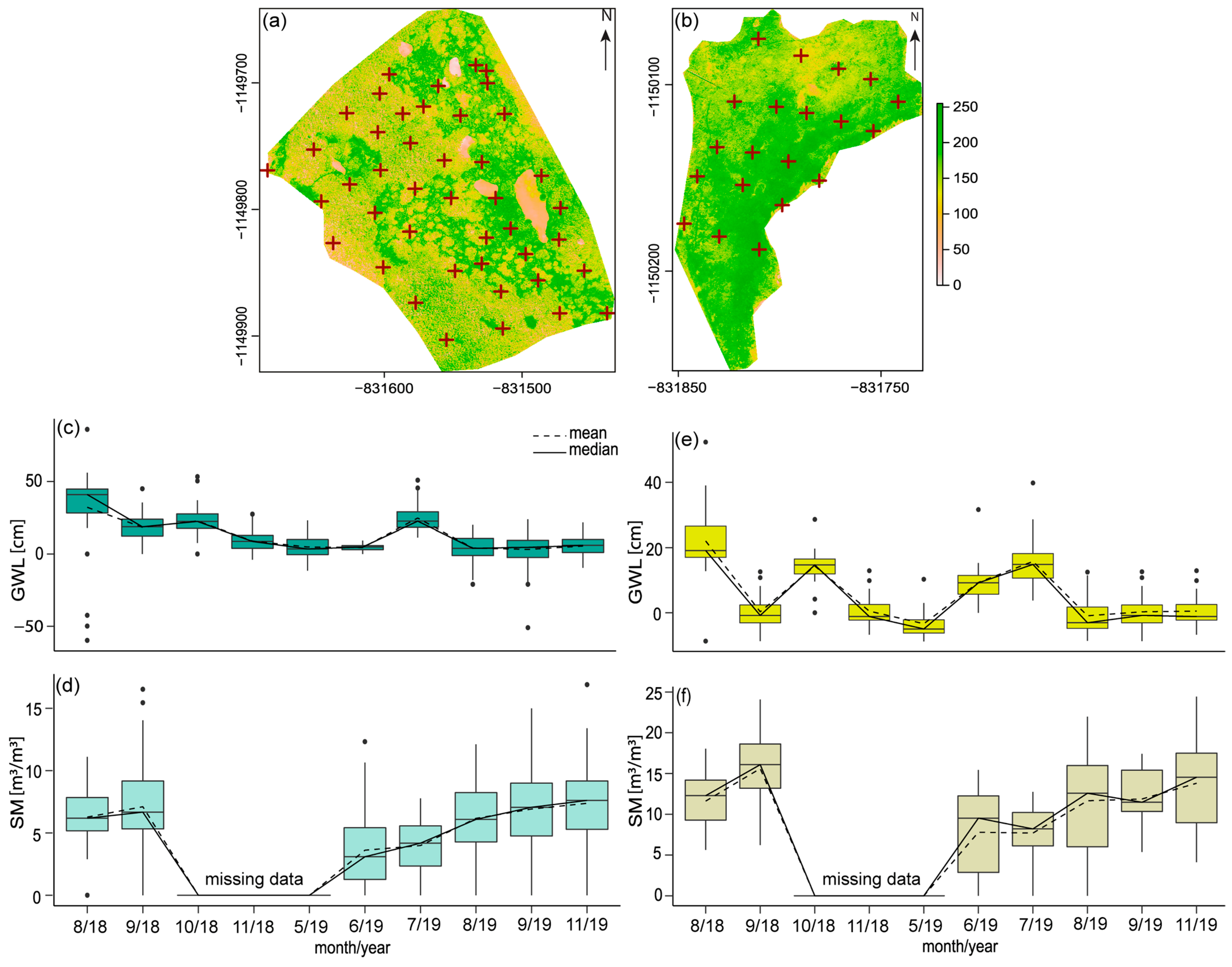
In this study, we distributed the water wells at two locations to measure GWL and SM by sampling them next to the wells (Figure 5), and the main aim was to predict GWL and SM based on a set of potential spatial and temporal predictors (34 predictors), which are terrain related, vegetation indices, or reflect surface thermal properties. Each of the wells represented a “Tube ID” (Figure 5a,b; red crosses).

Among the validation strategies, k-fold CV is popular to estimate the model’s performance because of data that have not been used for model training. During CV, models are repeatedly trained (k models), and with each model run, the data of one-fold are put to the side and are not used for model training but model validation. In this way, the performance of the model can be estimated. Typically, a random k-fold is used, which means that each of the folds contains the training data (i.e., to map GWL or SM) since we aimed to map GWL and SM instead of performing a target-oriented validation that validated the model in view to spatial mapping. We were not interested in the model performance given random subsets of our data locations, but we needed to know how well the model can predict areas without data loggers. To find this out, we needed to repeatedly leave the complete time series of one or more data locations and use them as test data during CV. To do this, we needed to create meaningful folds by using CAST’s function “CreateSpaceTimeFolds,” which is designed to provide index arguments used by caret’s trainControl, where the data samplings’ location defines a location. The index defined which data points were used for model training during each model run and reversely defined which data points were hindered. Thus, using the index argument, we could account for the data’s dependencies by leaving the complete data from one or more data locations out like in LLO CV. We focused on LLO CV; therefore, we used the “Tube ID” to define the location of a data location (water well) and split the data into five-folds; thus, five model runs were performed, each leaving one-fifth of all data loggers out for validation. Furthermore, CAST’s FFS variable selection was used to exclude counterproductive variables or will not improve the LLO performance and thus excluded from the model by FFS [33,59]. In that way, FFS selected variables led in combination with the highest LLO performance and the best spatial model. Consequently, FFS trained all possible pairs of two predictor variables, and the best predictor (hyperparameter settings) was used at the respective split to partition the data (mtry); thus, the optimal models with the smallest values. Based on these optimal models, predictor variables were iteratively increasing, and each of the remaining variables was tested for its improvement, reaching the best model. The variable importance is based on the out-of-bag MSE for an RF model [60]. The out-of-bag MSE is calculated for each tree before and after permuting a variable. The differences are averaged and normalized by the standard error. The importance scores were executed by the “varImp” function in R.

The LLO CV error must be deemed the final performance indicator of spatial and spatiotemporal models [32]. Based on the trained model values extracted by point shapefile at 63 tube locations, we made spatial predictions of GWL and SM on the raster stacks containing all predictor variables’ spatial data for that day of fieldwork. Thus, the trained model was used on these raster datasets, resulting in spatially comprehensive GWL and SM maps (Figure 6 and Figure 7). At first sight, the predictions maps look good, but how accurate are they?

To analyze if the predicted models applied to the entire study area or if there were locations that were different in their predictor properties, [33] developed an approach to make predictions over an area of interest, determine the best model variables, and simulate how accurately the prediction performs far beyond the sampling locations in the AOA. We used that analysis for the proposed monthly models across the study area if there are different locations in their predictor properties from what the model has learned. In short, the proposed method implements a unitless measure for expressing how different a new data point is from the training data set, the so-called DI, a measure of unknown space, which proposes a threshold to define the AOA of a model. Consequently, the AOA is calculated using the model validated by CV. Second, it takes the spatial clusters into account and determines the threshold based on minimum distances to the nearest training point not located in the same cluster. This is done in the AOA function, where the folds used for CV are automatically extracted from the model. For example, we used a five-fold CV for model validation. The training data were split into five-folds where one-fifth (one fold) of the training data was left out during CV. Based on that one-fold held back during CV, the DI is calculated to all the other training data samples that have not been located at the same CV fold. In this way, the DI distribution can be seen within the training data and taken as a threshold by assuming the CV error was based on these DIs in our training data. Is DI smaller than the threshold, the predicted area is inside the AOA. Is the DI higher than the threshold, the predicted area is outside the AOA.

Thus, two data sets were used; the proposed training sampling locations, which were already trained and made the first selection of the best variables by the FFS; and the second dataset, which contained the raster stacks (32, 33, or 34 layers) with the new locations where predictions were used. In the end, we obtained a raster showing us the AOA, the area for which we expected the mode to make reliable predictions (Section 3.2). For more details, see [33]. To determine if relationships between the predictive models and the ground truth data existed, we plotted the GWL and SM variability (mean and median) (Figure 5c–f) at both sites to assist the proposed interpretation.

3. Results

3.1. Predictive Outputs

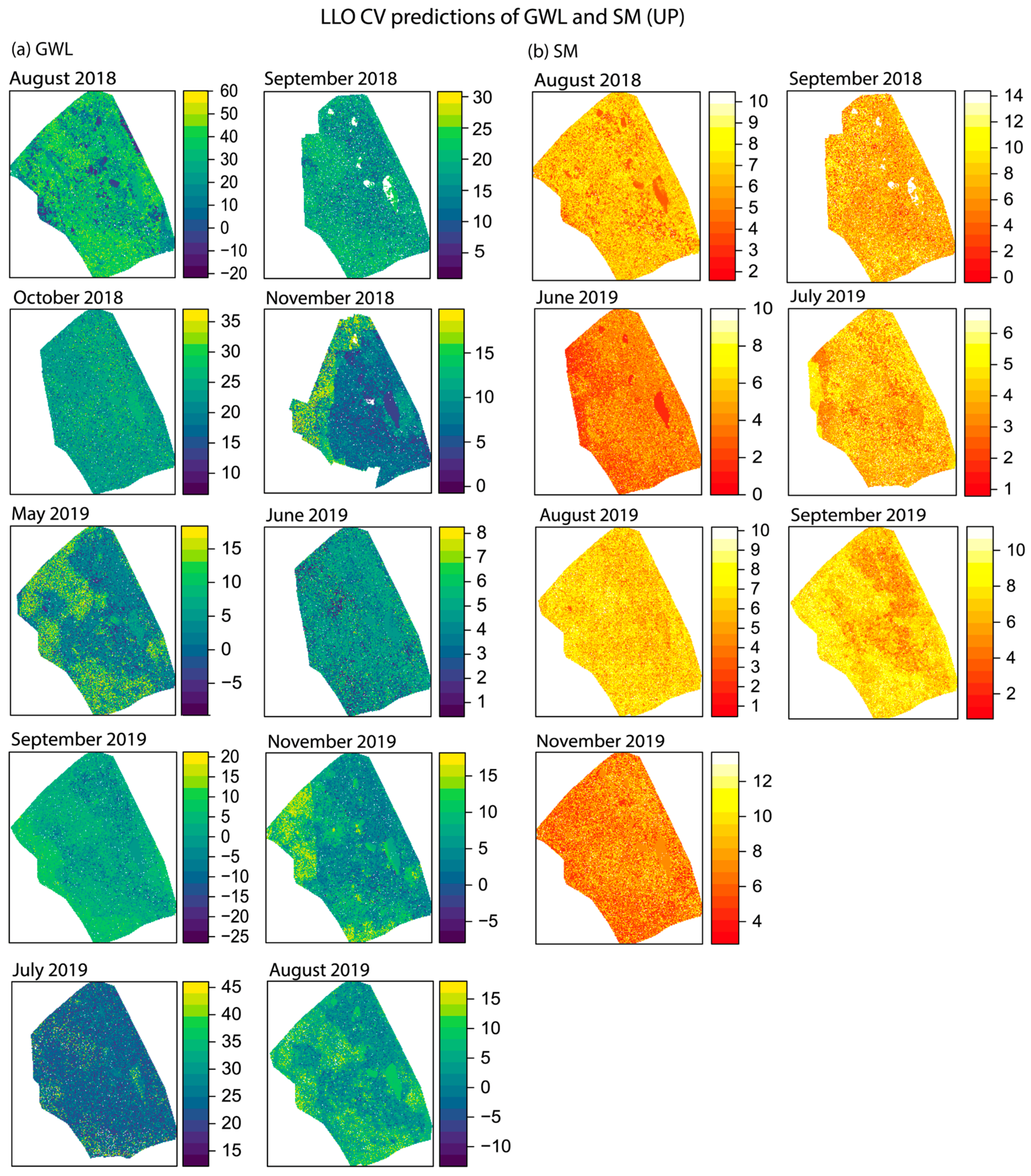
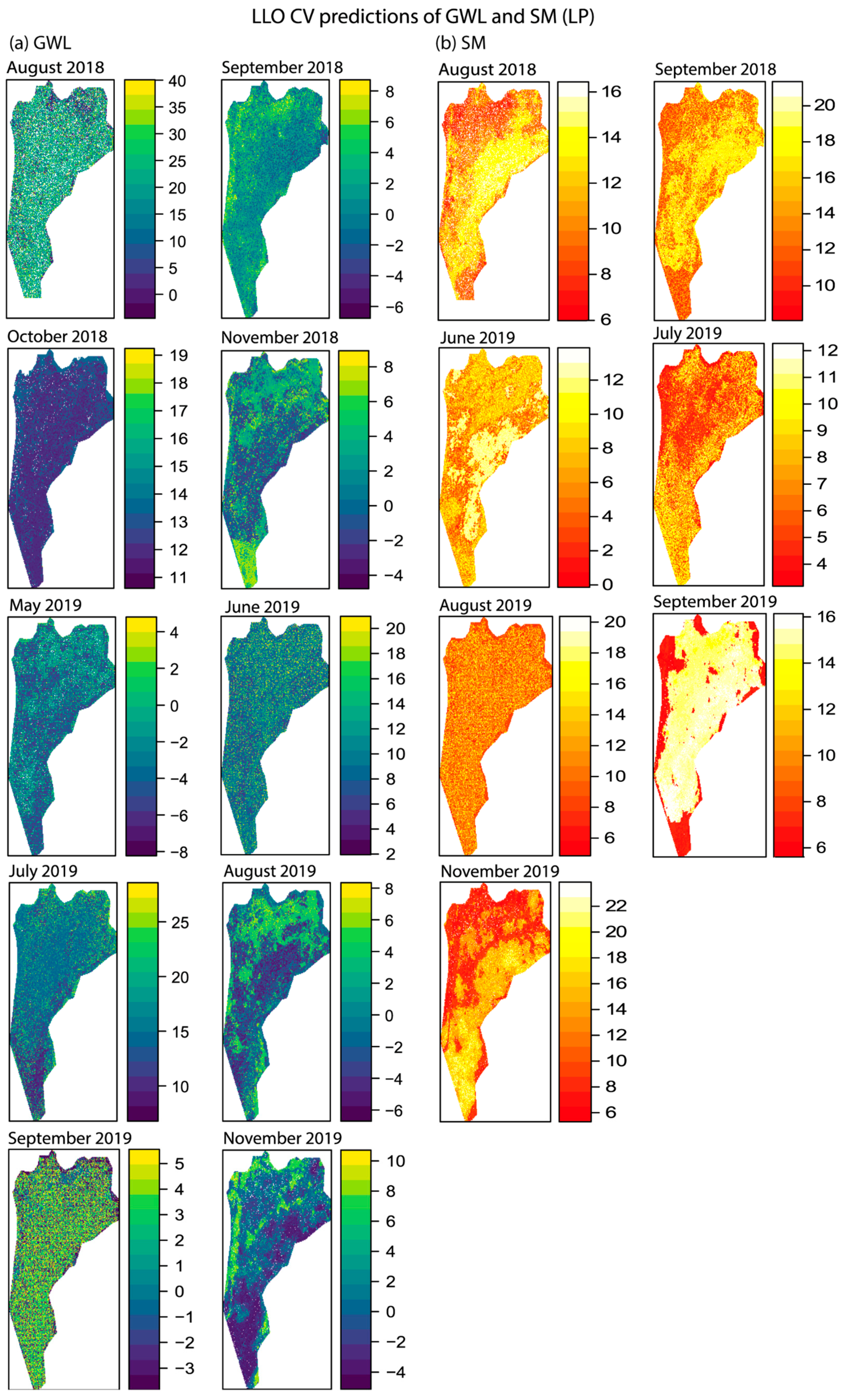
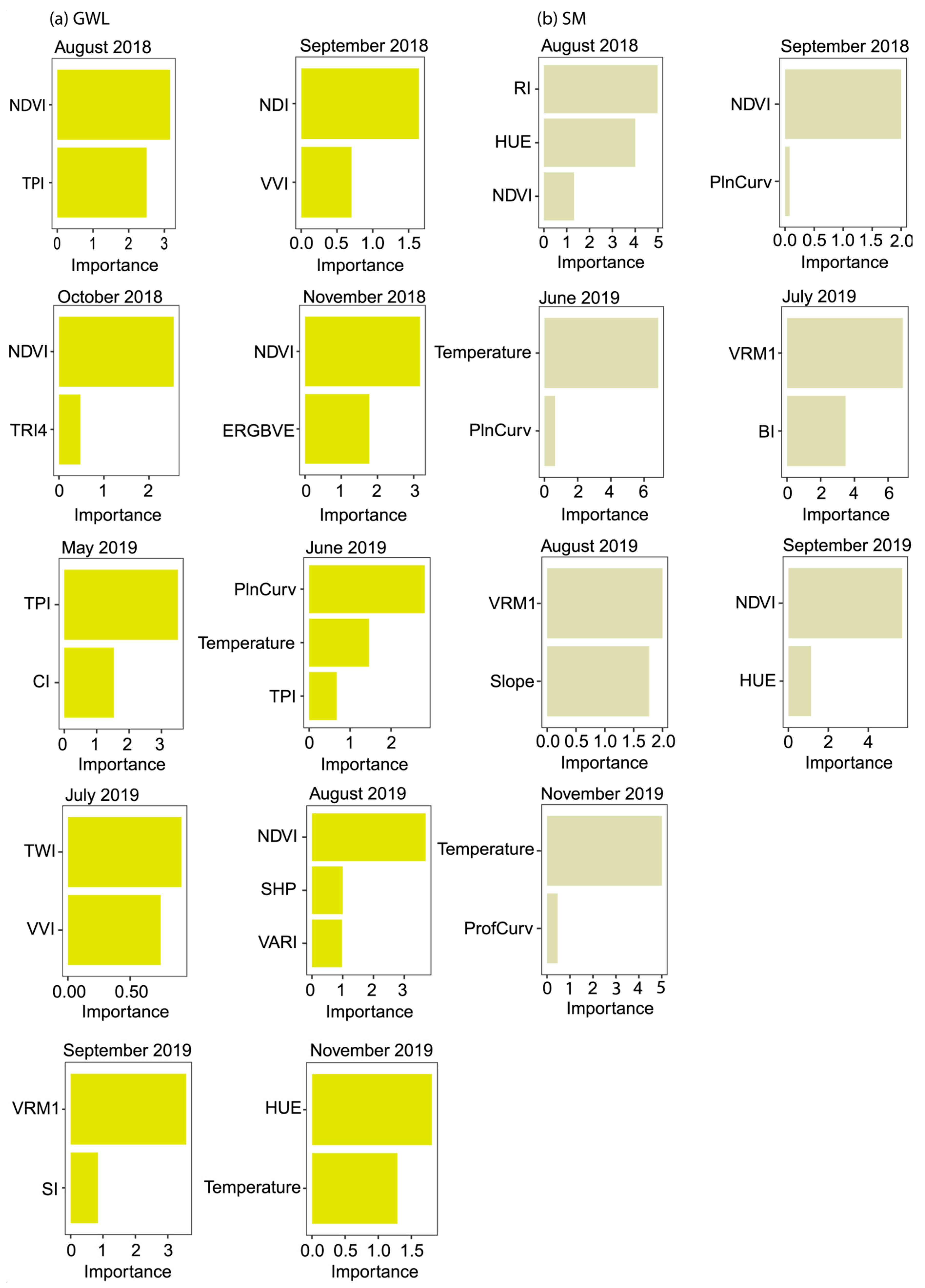
Figure 6 and Figure 7 show the individual simulated response predictions for GWL and SM’s respective pixels for the entire UP and LP using the root-mean-square error (RMSE) as the metric for the optimal variable selection using the smallest values. Despite the differences in the final set of variables selected, the spatial predictions of the GWL and SM at both sites led to different results. The RF regression models’ performance statistics, which only include variables selected in the FFS selection process, are shown in

Table 2. Statistical performance of the CAST models using cross-validation and a spatially constrained 5-fold based on the FFS method. Mtry value is the number of variables available for splitting at each model tree node. Model performance was assessed through the Root-Mean-Square-Error (RMSE), the Coefficient of Determination (R²), Mean Absolute Error (MAE), and their respective Standard Deviations (SD). Reference estimates were assessed through MEAN, MEDIAN, SD, and the average score (MEAN) for both GWL and SM models, and reference data.

Date	Location	Variables	mtry	RMSE	R2	MAE	RMSE_SD	R2_SD	MAE_SD	MEAN (ref.)	MEDIAN (ref.)	SD (ref.)
August 2018	UP	GWL	2	22.15	0.33	14.84	9.95	0.22	5.05	32.20	41.00	27.10
September 2018	UP	GWL	2	8.66	0.33	7.11	1.62	0.21	1.34	18.40	18.70	10.10
October 2018	UP	GWL	2	10.32	0.13	7.65	3.50	0.15	2.36	22.70	22.40	10.80
November 2018	UP	GWL	2	7.52	0.18	5.79	1.07	0.18	0.92	8.99	8.70	7.82
May 2019	UP	GWL	2	6.64	0.42	5.21	1.44	0.21	1.18	4.86	3.50	8.05
June 2019	UP	GWL	2	1.96	0.32	1.59	0.67	0.12	0.55	4.50	4.84	2.31
July 2019	UP	GWL	2	7.57	0.23	6.41	1.71	0.24	1.16	24.70	22.60	8.74
August 2019	UP	GWL	3	7.65	0.43	5.72	1.85	0.20	1.44	4.16	4.00	9.64
September 2019	UP	GWL	2	9.92	0.41	7.32	4.00	0.24	1.66	3.19	4.60	12.70
November 2019	UP	GWL	2	6.05	0.36	4.97	0.79	0.33	0.54	5.51	6.00	7.27
Average score (MEANGWL_UP)				8.84	0.31	6.66	2.66	0.21	1.62	12.92	13.63	10.45
August 2018	LP	GWL	2	6.46	0.78	5.69	5.79	0.16	5.01	22.00	19.10	12.20
September 2018	LP	GWL	2	5.36	0.46	4.79	3.92	0.45	3.61	0.31	−0.80	5.65
October 2018	LP	GWL	2	5.44	0.46	4.12	2.05	0.44	1.45	14.40	14.70	5.83
November 2018	LP	GWL	2	4.32	0.56	3.62	2.16	0.29	1.70	0.52	−1.15	5.28
May 2019	LP	GWL	2	4.09	0.34	2.96	1.51	0.35	0.72	-3.35	−4.95	4.58
June 2019	LP	GWL	2	6.03	0.47	4.71	2.24	0.49	1.40	9.32	9.20	6.85
July 2019	LP	GWL	2	8.10	0.30	5.69	4.20	0.32	2.39	15.80	14.80	8.23
August 2019	LP	GWL	2	4.05	0.73	3.40	3.21	0.26	2.41	-0.91	−3.05	6.02
September 2019	LP	GWL	2	4.46	0.53	3.68	1.91	0.39	1.80	0.31	−0.80	5.65
November 2019	LP	GWL	2	5.89	0.13	4.58	1.24	0.14	1.15	0.52	−1.15	5.28
Average score (MEANGWL_LP)				5.42	0.48	4.32	2.82	0.33	2.16	5.89	4.59	6.56
August 2018	UP	SM	2	2.60	0.12	2.09	0.46	0.10	0.27	6.27	6.18	27.10
September 2018	UP	SM	2	3.24	0.28	2.71	0.58	0.22	0.29	7.10	6.67	10.10
June 2019	UP	SM	2	2.83	0.12	2.34	0.91	0.12	0.56	3.61	3.09	2.31
July 2019	UP	SM	2	1.73	0.29	1.48	0.53	0.22	0.39	3.99	4.18	8.74
August 2018	UP	SM	2	2.85	0.41	2.30	0.61	0.38	0.48	6.17	6.09	9.64
September 2018	UP	SM	2	2.82	0.22	2.31	0.42	0.17	0.39	6.92	7.06	12.70
November 2018	UP	SM	2	3.35	0.33	2.56	0.91	0.17	0.80	7.38	7.61	7.27
Average score (MEANSM_UP)				2.77	0.25	2.26	0.63	0.20	0.45	5.92	5.84	11.12
August 2018	LP	SM	2	2.42	0.48	2.06	0.72	0.37	0.67	11.60	12.30	12.20
September 2018	LP	SM	2	3.96	0.45	3.56	2.01	0.42	1.92	15.60	16.10	5.65
June 2019	LP	SM	2	3.33	0.52	2.71	1.77	0.32	1.43	7.79	9.52	6.85
July 2019	LP	SM	2	2.77	0.55	2.37	0.94	0.30	0.60	7.69	8.20	8.23
August 2018	LP	SM	2	5.83	0.21	4.77	1.17	0.26	0.82	11.70	12.60	6.02
September 2018	LP	SM	2	2.59	0.59	1.99	0.96	0.41	0.48	11.90	11.50	5.65
November 2018	LP	SM	2	5.32	0.47	4.30	1.95	0.17	1.93	13.80	14.50	5.28
Average score (MEANSM_LP)				3.75	0.47	3.11	1.36	0.32	1.12	11.44	12.10	7.13
Average score (MEANall)				5.54	0.38	4.34	2.02	0.27	1.44	9.11	9.05	8.76

. GWL spatial predictions typically resulted in higher RMSE values but not necessarily in lower response variable predictions, as shown by the R² values (Table 2). The best fit model for GWL prediction occurred in August 2019 (R² = 0.43) at the UP and in August 2018 at the LP (R² = 0.78). In comparison, SM spatial predictions resulted in lower RMSE values but showed a lower prediction power at both sites. The best fit model of the simulated SM prediction occurred in August 2019 (R² = 0.41) at the UP and in September 2019 at the LP (R² = 0.59). The importance of the different predictors ranged from 0 to 8 (GWL at UP), 0 to 5 (SM at UP), 0 to 3 (GWL at LP), and 0 to 5 (SM at LP) (Figure 8 and Figure 9). These ranges represent the baseline for the variable weighting used to estimate the DI. The essential relative variables or feature importance ranking of RF for GWL predictions were temperature, RGB spectral variables (BI, GLI, CI, RI, and HUE), and one topomorphometric feature (TWI) at the UP (Figure 7). Conversely, the LP importance variables for GWL predictions were NDVI, topomorphometric variables (PlnCurv, TWI, VRM1, and TPI), and, to a lower degree, RGB spectral variables (HUE and NDI) (Figure 9). The importance of predictive variables for the SM simulated prediction were mainly RGB spectral variables (BI, HI, ERGBVE, SHP, and HUE), NDVI and temperature at the UP and temperature, NDVI, topomorphometric predictor (VRM1), and RGB spectral variable (RI) at the LP (Figure 8 and Figure 9).

3.2. AOA Calculations

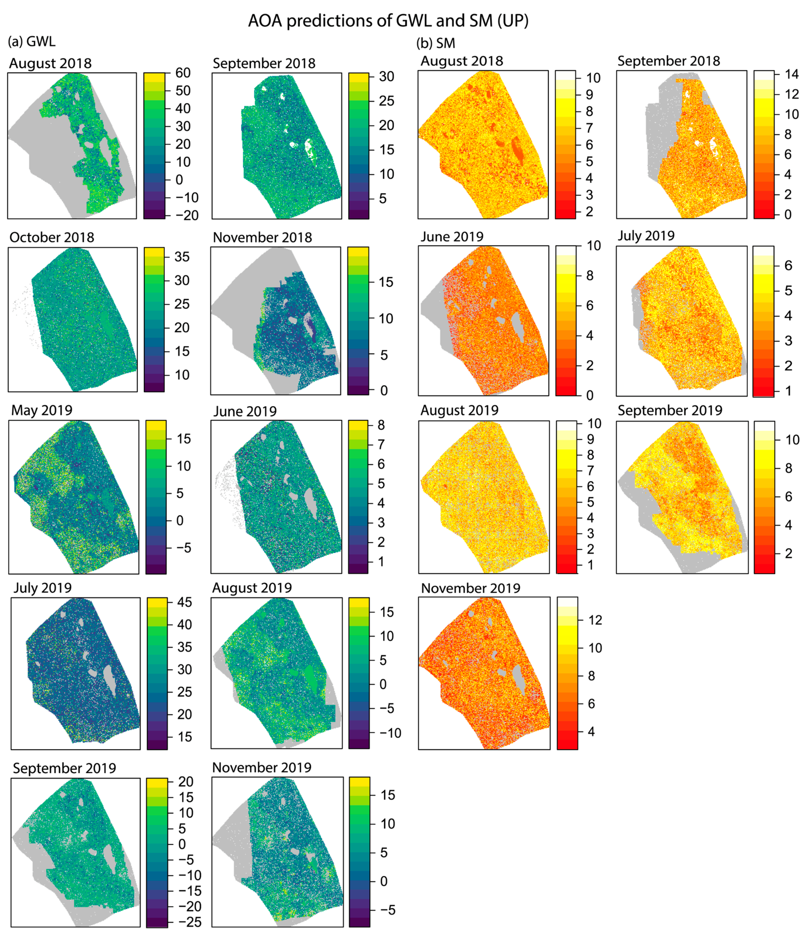
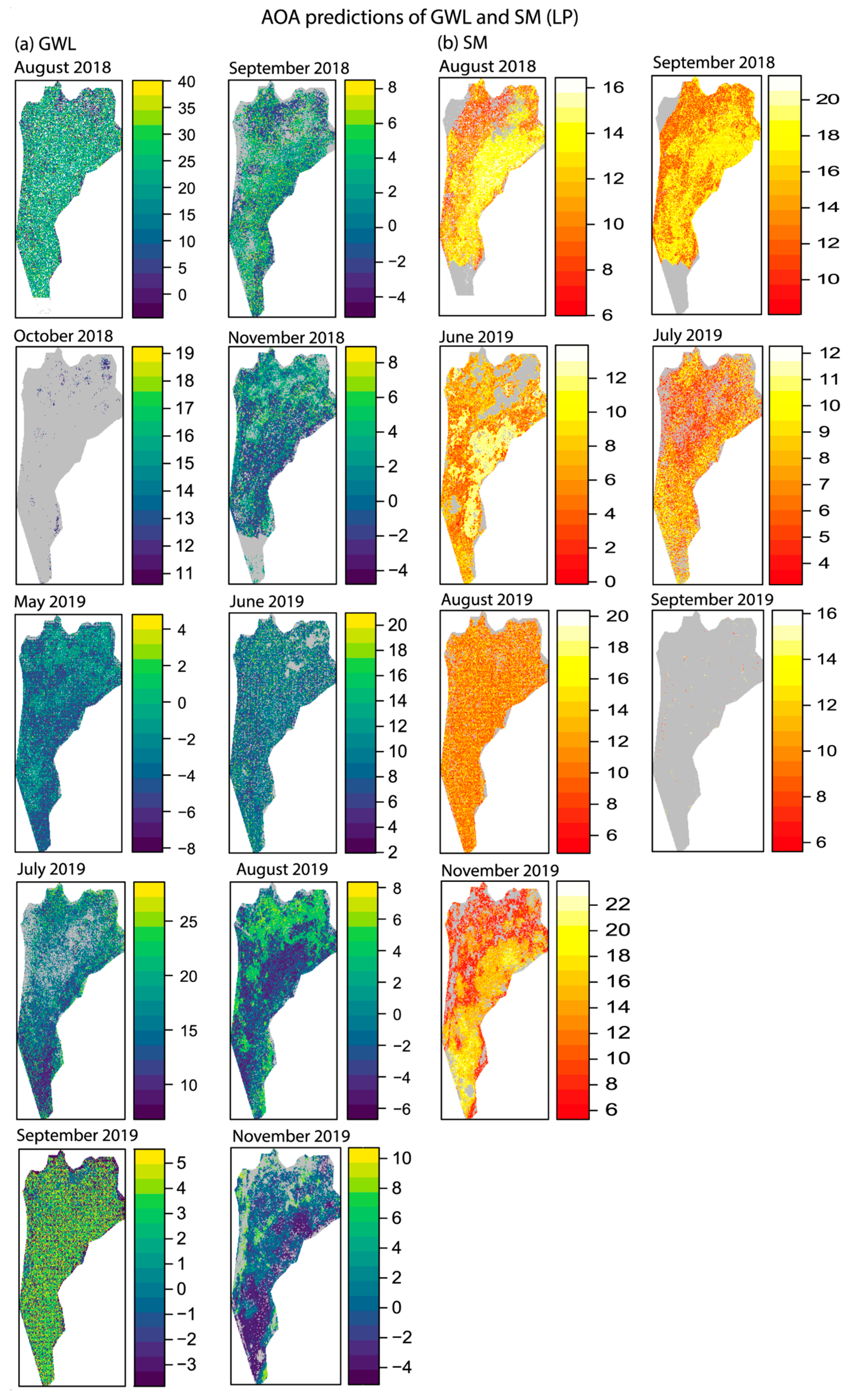
The accuracies of model predictions were determined using AOA calculations. The AOA areas for which we expected the model to make reliable predictions are shown in Figure 9 and Figure 10. AOA simulation models used the 95% quantile of the DI of all training data as a threshold suggested by [33], where the DI of the training data is calculated by considering the CV folds in the 5 fold case. Applying this threshold, the prediction error (RMSE) inside the AOA should be comparable to the trained model’s CV RMSE. Conversely, the CV error does not apply outside the AOA [33]. Most simulated predictions showed reliable predictions (less of a gray area) except for a few (e.g., August 2018 and November 2018 for GWL and September 2018 for the SM simulation at the UP; Figure 10), where most areas were outside the AOA (gray area). Thus, predictions should not be considered for these locations or in further analysis. Reliable predictions were also made for the LP (Figure 11), except for October 2018 (GWL prediction) and for September 2019 (SM prediction), where the entire area is nearly gray. In future analysis, these two months might not be counted. Typically, low applicability values at the UP site appeared at the bush sites, over water surfaces, and at the corners and edges of the study area (Figure 10). A LP site, low applicability values emerged between the high grass or the area edges (Figure 11).

As a real-world example, we could not analyze the AOA reliability with simulated data [32,59,61,62,63,64], where the prediction error within the AOA can be compared to the model error, assuming that the model error applies inside the AOA but not outside. Therefore, a simulated area-wide response is not available in usual prediction tasks; therefore, the AOAs estimation in the dataset used in this study had only point observations as a reference. We plotted the relationship between the DI threshold derived by the 95 quantile and the relative prediction performance measurements (Figure 12a,b).

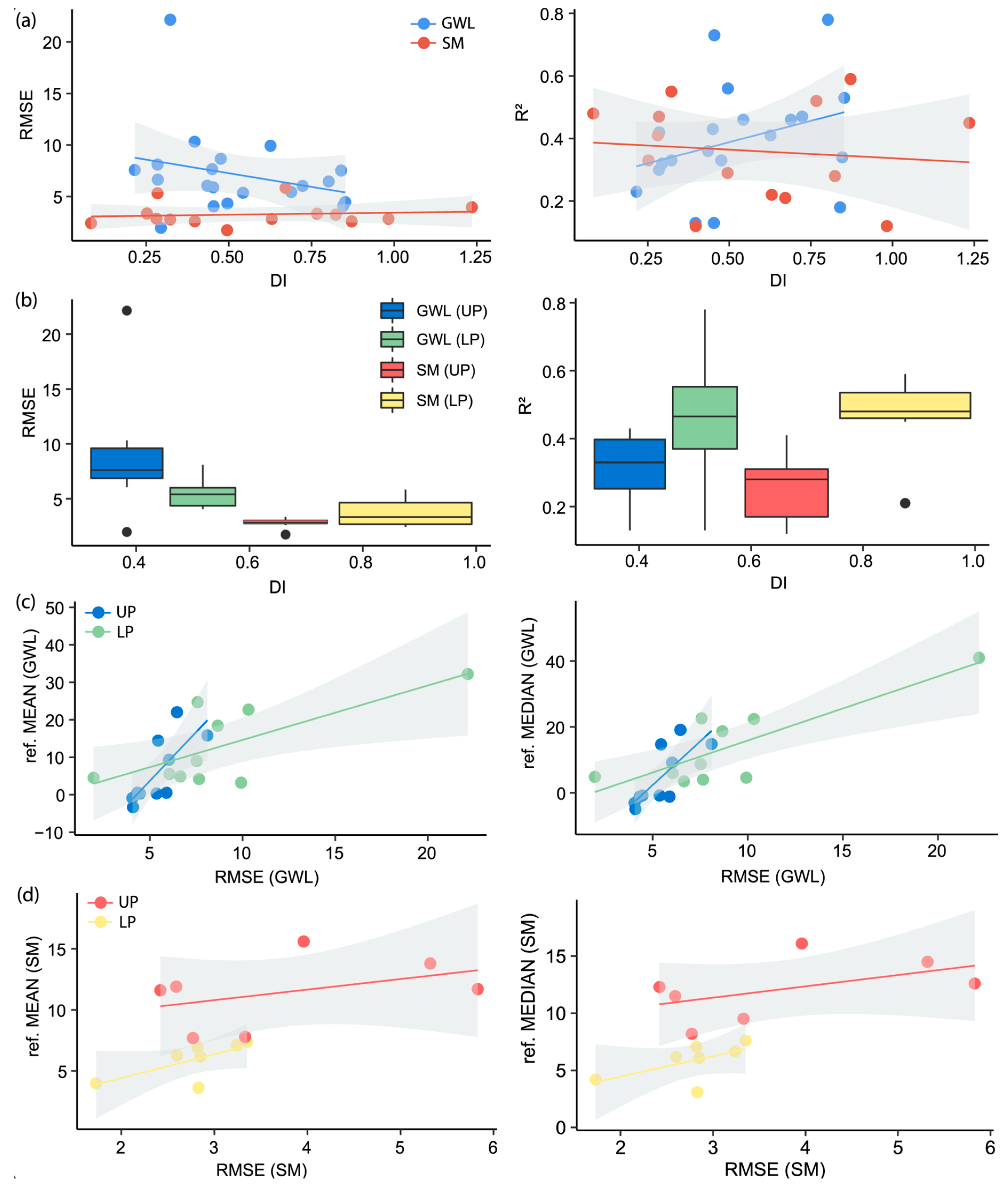
DI provides a basis to estimate the AOA that allows the area for which the CV is suited accurately on average. Based on [33], if a location is similar to the training data properties, it will have a low distance in the predictor variable space (DI towards 0), while locations that are significantly different in their properties will have a high DI. DI threshold values differed between the GWL and SM predictions (Figure 12a). The GWL DIs were lower and more robust, ranging from 0.22 to 0.85, but were caused by higher predicted RMSE. Conversely, SM DIs were more widespread (0.084–1.23) and probably more sensitive, resulting in lower predicted RMSE values (Figure 12a). It was also optimistically approved by R² estimates, showing higher R² for higher GWL DIs and vice versa (Figure 12a). The R² for SM estimates resulted in a slighter opposite trend showing higher SM DIs by lower R² estimates. Individually, as observed in the boxplots, the GWL prediction models showed the highest absolute RMSE errors at lower DI thresholds at the UP, in which the lowest RMSE performances were at moderate to high DIs for the SM models at the UP and LP, respectively (Figure 12b). The best relative (R²) model performances were made for the SM and GWL models at the LP with the highest DIs (Figure 12b) The statistical relationship between field data and the absolute model performances indicated a trend that by lower GWLs and higher surface water, the predicting models resulted in better prediction performances at both sites (Figure 12c). A similar trend was seen for the SM field data and their model performances, showing the models’ lower SM better achievements (Figure 12d). The best model performances result in environmental conditions with relatively low GWL and SM than those to higher GWL and SM events (Figure 12c,d).

4. Discussion

4.1. Model Performance

Overall, using the CAST prediction method of implementing the FFS in conjunction with target oriented LLO CV validation, modeling GWL and SM was probably not the best way to provide highly accurate prediction maps with high R² and low RMSEs. However, the proposed method preserved the modeling results with regard to overfitting and objective error assessment, a common problem in ML [32,59]. Thus, we did not consider longitude, latitude, and elevation as predictors that are typically responsible for overfitting due to spatiotemporal autocorrelation patterns stated in [32] that would probably result in better model performances. We only focused on the FFS’s environmental predictors to minimize overfitting and retain the data’s real spatiotemporal independencies (nonlinear and complex system), which is challenging to interpret physically by obtaining information on a handful of environmental variables in space and time.

By evaluating all RF performances (highest R², lowest RMSE), we achieved the best results with the GWL and SM at the LP site, and the lowest variation in the predictions were found at the UP site. As a potential reason, lower performance might be caused by the test data, including, incomplete spatial coverage of the mapping area [65] and, more likely, incomplete coverage of the UAV maps. UAV mapping of an entire study area cannot be maintained constantly during field campaigns due to wind, battery, or camera failures, particularly for the Tetracam camera, which is sensitive to operational conditions. From the AOA predictions at the UP site, it is clear to move the sampling strategy from the bush site only to the open sites with grass, moss, and bare peat patches. Additionally, surface water is more easily viewed when the soil at the open sites is thoroughly saturated with water directly after precipitation or after snowmelt (e.g., May 2019, June 2019, August 2019, September 2019, November 2019), which is the primary source of extra inflow water to the peat bog. The remaining months (e.g., August 2018, October 2018, September 2018, July 2019) were less saturated, or the surface (bare peat patches) appeared to be nearly dry, especially at the UP (Figure 4).

In comparison, the LP site seemed to provide better GWL prediction. Most likely because the LP was saturated with water most of the time (Figure 4), the homogenous cover acted like a sponge and retained daily rainfall. In general, the lower the GWL level of the peat bog area is, the higher the surface water saturation and vice versa. This fact describes the dual-porosity organic soils [66,67]. Groundwater fluctuates in larger peat pores filled with mobile water. Undecomposed tissues of organic materials contain a nonnegligible volume of immobile water. Moreover, groundwater tables in tubes are affected by gravity rather than capillary forces in small capillary pores. These forces oppose each other, particularly during dry periods. However, this is not always the case due to other impacts, such as runoff, evaporation [68], and physical soil properties, such as peat volume change [69] or repellency [70]. Repellency can also affect the soil moisture distribution even several cm below the soil surface. The UP’s surface runoff influences the LP; thus, the LP site was frequently flooded by water, resulting in lower and more diverse GWL measurements (Figure 4e), while the GWL in the UP was higher and relatively steady (Figure 5c).

As mentioned above, SM predictions were marginally better at the LP than at the UP, which might be caused by homogenous vegetation cover and the marginally higher SM values measured at UP. Vegetation cover is known to play a vital role in the hydrometeorological cycle and local climate conditions [71]. Wet conditions, such as those at the LP, with high grass coverage and frequent saturated surface water along with heat energy are required to increase the soil temperature because water has a higher specific heat capacity than soil material, leading to an increase in SM and likely a better response to wetting and drying cycles, improving SM prediction [72]. The high variety of the SM DIs, which ranged widely, might be more sensitive to environmental factors than the GWL predictions, which showed more robust DI distributions (Figure 12a). This hypothesis, however, is part of the measurement in another experiment.

4.2. Interpretation of Model Predictions

Surface temperature is the most important predictor for the GWL and SM at both the UP and LP with regard to model importance. Surface temperature influences water movement in the soil: the higher the surface temperature is, the higher the evaporation of soil water. Organic soils are more resistant to evaporation, which is primarily caused by increasing temperature [73], for several reasons, including disconnection temperature conductivity during the drying process. However, transpiration can substitute for the loss of water from a peat bog. Hypothetically, a temperature rise in the future and water holding (the GWL) might be affected by higher transpiration. The GWL is considerably dynamic, and ombrotrophic bogs, such as the proposed experimental study area, are dependent on precipitation, which typically describes the high variability of the GWL [15]. Ref. [10] suggested that the GWL is specially controlled by the difference between precipitation and evapotranspiration, as stated in [14,74]. The temperatures of the surface water and GWL are affected by the amount of incoming solar radiation and the vegetation pattern. For example, the exposed bare peat patches absorb more heat in the UP, resulting in a rapid decrease in GWL and increased water temperature [15] when the peat is not dry with a high-temperature conductivity. Spots with higher temperatures aid water tracking and hydrograph separation. Beyond confirming the temperature–GWL–SM relationship, the RF provided insight into the usefulness and the impact of NDVI, as well as RGB spectral indices (BI, CI, GLI, RI, HUE, NDI, SHP, and ERGBVE), directly representing proxies for the estimation of vegetation response towards changes in hydroclimatic conditions [53,75,76]. Moreover, these predictors can be considered appropriate for assessing vegetation conditions in peatlands to characterize temporal and spatial patterns and the degradation process of a peat bog ecosystem [77], primarily NDVI, NDI, ERGBVE, SHP, and GLI. Interestingly, the predictors BI, CI, RI, and HI are important; thus, there seems to be a relationship between these factors, GWL and SM. Typically, these predictors are more prone to bare soil (in this study, bare peat coverage) and may provide accessory information about soil physical properties (e.g., about peat composition due to a lower water table during dry periods) [78]. Because SM decreases on a typically decomposed peat surface, high soil water retention may develop and yield development that has already been observed at the UP site. However, further investigations are required to clarify this specifically.

Further, the UP site contained the highest number of topomorphometric variables (TWI, PlnCurv, TPI, and VRM1) for GWL predictions and twice the number for SM predictions (VRM1) at the LP. The TWI is a measure of subsurface lateral transmissivity and has become a familiar and widely used method to gather information about the spatial distribution of wetness conditions (e.g., the position of shallow groundwater tables and soil moisture) [79]. PlnCurv, TPI, and VRM1 are topographic indices and thus play a significant role in GWL predictions with regard to dominant controls on groundwater level and runoff mechanisms [80]. Small local hydraulic gradients might control the downslope drainage condition, which determines GWLs [80]. As reported in [81], the probability of sphagnum decreases with increased ruggedness, elevation, and topographic position, which provides information on exposed bare peat. As reported in [82], VRM1 contributes to SM, particularly when using high-resolution DEMs; thus, VRM1 is a suitable proxy for soils with different porosities in terms of high roughness, highlighting that stony soils imply low soil moisture, and that low roughness describes developed soils that retain more moisture, as in peat. VRM1 measures vector dispersion across the central pixel rather than being a derivative of the slope, and is thus a much better proxy than others, such as TRI [83].

The proposed predictive models identify a variety of RGB, multispectral, and thermal maps as well as DSM-derived variables as suitable or complementary representatives to in situ measurements for GWL and SM predictions. However, we recommend going beyond their traditional use of, for example, elevation, slope, and aspect. Additionally, these derived variables, such as the RGB spectral indices and DSM-derived ones, are easy to compute proxies of environmental features that involve limited fieldwork and good knowledge of the peat bog’s environmental peat bog status.

5. Conclusions

We tested how well the peat bog groundwater level (GWL) and soil moisture (SM) can be predicted using multi-source and multitemporal ultrahigh-resolution UAV maps with leave-location-out (LLO) cross-validation (CV) prediction models based on random forest (RF) machine learning (ML) algorithm. Additionally, forward feature selection (FFS) was used to prevent overfitting, and only the optimal predictor variables were used for spatial and temporal model predictions. In this case study, the predicted GWL and SM maps used 34 possible candidate predictors to visualize and access knowledge about the dynamic properties of two different peat bog locations in the Rokytka Moors within Sumava NP, Czechia. As input data, we used RGB spectral indices (RGI, VVI, VDVI, VARI, TGI, SI, SHP, SCI, SAT, NGRDI, NDTI, NDI, HI, GRVI, GLI, GLAI, ExG, ERGBVE, CI, BI, RI, and HI) and NDVI from multispectral data to obtain the vegetation response to changes in hydroclimatic conditions. We selected temperature soil information based on thermal data to explore the thermal potential on GWL and SM and topomorphometric variables (Slope, ProfCurv, PlnCurvc, WEI, TRI, VRM, TPI, and TWI) derived from DSMs to investigate microtopomorphometric controls on GWL and SM patterns. The created maps had a spatial resolution of 0.03 × 0.03 m. Predictions of the variable importance have proven the dominant impact of temperature on GWL and SM and extremely significant contributions of other predictors, such as NDVI, NDI, ERGBVE, SHP, GLI, BI, CI, RI, HI, TWI, PlnCurv, TPI, and VRM1. The predictions resulted in low (lowest R² = 0.12) to high (highest R² = 0.78) CV performances. We also mapped the area of applicability (AOA) of spatial prediction models (i.e., the area in which a model could expect to make accurate predictions). Prediction outside the AOA should be treated with caution. Most of the proposed predicted models yielded acceptable models except for a few where the incomplete spatial coverage of UAV maps was missing, and nearly all these areas were outside of the AOA. Primarily, ground truth sampling can be avoided in bush areas. The results showed that the DSM, RGB, multispectral, and thermal UAV imaging datasets were important in GWL and SM estimations to predict spatial distribution phenomena, especially the best model performances resulting in environmental conditions with relatively low GWL and SM than those to higher GWL and SM events. Thus, further research is needed both in sampling more ground measurements and in using additional profound statistical procedures to understand the causal structure of its underlying phenomena or interpretation of the ML models using UAV data. It is advisable to combine UAV input data with many relevant environmental variables used in this study when studying the dynamic mapping properties in spatially heterogeneous peat bog landscapes.

References

- Grzybowski, M.; Glińska-Lewczuk, K. The Principal Threats to the Peatlands Habitats, in the Continental Bioregion of Central Europe—A Case Study of Peatland Conservation in Poland. J. Nat. Conserv. 2020, 53, 125778. [Google Scholar] [CrossRef]
- Keddy, P.A. Wetland Ecology: Principles and Conservation, 2nd ed.; Cambridge University Press: Cambridge, UK, 2010; ISBN 978-0-511-77817-9. [Google Scholar]
- Holden, J.; Wallage, Z.E.; Lane, S.N.; McDonald, A.T. Water Table Dynamics in Undisturbed, Drained and Restored Blanket Peat. J. Hydrol. 2011, 402, 103–114. [Google Scholar] [CrossRef]
- Spitzer, K.; Danks, H.V. Insect Biodiversity of Boreal Peat Bogs. Annu. Rev. Entomol. 2006, 51, 137–161. [Google Scholar] [CrossRef]
- Bates, P.D.; Neal, J.C.; Alsdorf, D.; Schumann, G.J.-P. Observing Global Surface Water Flood Dynamics. Surv. Geophys. 2014, 35, 839–852. [Google Scholar] [CrossRef]
- Kocum, J.; Oulehle, F.; Janský, B.; Bůzek, F.; Hruška, J.; Vlček, L. Geochemical Evidence for Peat Bog Contribution to the Streamflow Generation Process: Case Study of the Vltava River Headwaters, Czech Republic. Hydrol. Sci. J. 2016, 61, 2579–2589. [Google Scholar] [CrossRef] [Green Version]
- Schreiber, H. Moore des Böhmerwaldes und des Deutschen Südböhmen; 4. Band der Moorerhebungen des Deutsch-Österreichischen Moorvereins; Verlag des Deutschen Moorvereines in der Tchechoslowakei: Sebastiansberg, 1924. [Google Scholar]
- Bufková, I.; Stíbal, F.; Mikulášková, E. Restoration of Drained Mires in the Šumava National Park, Czech Republic. In Wetlands: Ecology, Conservation and Management, Restoration of Lakes, Streams, Floodplains, and Bogs in Europe; Eiseltová, M., Ed.; Springe: Dordrecht, The Netherlands, 2010; Volume 3, pp. 331–354. ISBN 978-90-481-9264-9. [Google Scholar]
- Bufková, I.; Prach, K. Linking Vegetation Pattern to Hydrology and Hydrochemistry in a Montane River Floodplain, the Šumava National Park, Central Europe. Wetl. Ecol. Manag. 2006, 14, 317–327. [Google Scholar] [CrossRef]
- Vlček, L.; Kocum, J.; Janský, B.; Šefrna, L.; Kučerová, A. Retention potential and hydrological balance of a peat bog: Case study of Rokytka Moors, Otava River headwaters, sw. Czechia. Geografie 2012, 117, 395–414. [Google Scholar] [CrossRef]
- Vlček, L.; Kocum, J.; Janský, B.; Šefrna, L.; Blažková, Š. Influence of Peat Soils on Runoff Process: Case Study of Vydra River Headwaters, Czechia. Geografie 2016, 121, 235–253. [Google Scholar] [CrossRef]
- Vlček, L.; Falátková, K.; Schneider, P. Identification of Runoff Formation with Two Dyes in a Mid-Latitude Mountain Headwater. Hydrol. Earth Syst. Sci. 2017, 21, 3025–3040. [Google Scholar] [CrossRef] [Green Version]
- Vlček, L.; Šípek, V.; Kofroňová, J.; Kocum, J.; Doležal, T.; Janský, B. Runoff Formation in a Catchment with Peat Bog and Podzol Hillslopes. J. Hydrol. 2020, 125633. [Google Scholar] [CrossRef]
- Doležal, T.; Vlček, L.; Kocum, J.; Janský, B. Evaluation of the Influence of Mountain Peat Bogs Restoration Measures on the Groundwater Level: Case Study Rokytka Peat Bog, the Šumava Mts., Czech Republic. AUC Geogr. 2017, 52, 141–150. [Google Scholar] [CrossRef] [Green Version]
- Doležal, T.; Vlček, L.; Kocum, J.; Janský, B. Hydrological Regime and Physico-Chemical Water Properties of Various Types of Peat Bog Sites: Case Study of Mezilesní Peat Bog, Šumava Mts. Geografie 2020, 125, 21–46. [Google Scholar] [CrossRef]
- Kubatova, A.; Prasil, K.; Vanova, M. Diversity of Soil Microscopic Fungi on Abandoned Industrial Deposits. Cryptogam. Mycol. Fr. 2002, 23, 205–219. [Google Scholar]
- Sipek, M.; Perčin, A.; Zgorelec, Ž.; Sajna, N. Morphological Plasticity and Ecophysiological Response of Ground Ivy (Glechoma Hederacea, Lamiaceae) in Contrasting Natural Habitats within Its Native Range. Plant Biosyst. Int. J. Deal. Asp. Plant Biol. 2021, 155, 136–147. [Google Scholar] [CrossRef]
- Wallace, L.; Lucieer, A.; Watson, C.; Turner, D. Development of a UAV-LiDAR System with Application to Forest Inventory. Remote Sens. 2012, 4, 1519–1543. [Google Scholar] [CrossRef] [Green Version]
- Lehmann, J.; Nieberding, F.; Prinz, T.; Knoth, C. Analysis of Unmanned Aerial System-Based CIR Images in Forestry—A New Perspective to Monitor Pest Infestation Levels. Forests 2015, 6, 594–612. [Google Scholar] [CrossRef] [Green Version]
- Rahman, M.M.; McDermid, G.J.; Strack, M.; Lovitt, J. A New Method to Map Groundwater Table in Peatlands Using Unmanned Aerial Vehicles. Remote Sens. 2017, 9, 1057. [Google Scholar] [CrossRef] [Green Version]
- Lovitt, J.; Rahman, M.; McDermid, G. Assessing the Value of UAV Photogrammetry for Characterizing Terrain in Complex Peatlands. Remote Sens. 2017, 9, 715. [Google Scholar] [CrossRef] [Green Version]
- Lovitt, J.; Rahman, M.M.; Saraswati, S.; McDermid, G.J.; Strack, M.; Xu, B. UAV Remote Sensing Can Reveal the Effects of Low-Impact Seismic Lines on Surface Morphology, Hydrology, and Methane (CH4) Release in a Boreal Treed Bog. J. Geophys. Res. Biogeosciences 2018, 123, 1117–1129. [Google Scholar] [CrossRef] [Green Version]
- Harvey, M.C.; Hare, D.K.; Hackman, A.; Davenport, G.; Haynes, A.B.; Helton, A.; Lane, J.W.; Briggs, M.A. Evaluation of Stream and Wetland Restoration Using UAS-Based Thermal Infrared Mapping. Water 2019, 11, 1568. [Google Scholar] [CrossRef] [Green Version]
- Isokangas, E.; Davids, C.; Kujala, K.; Rauhala, A.; Ronkanen, A.-K.; Rossi, P.M. Combining Unmanned Aerial Vehicle-Based Remote Sensing and Stable Water Isotope Analysis to Monitor Treatment Peatlands of Mining Areas. Ecol. Eng. 2019, 133, 137–147. [Google Scholar] [CrossRef]
- Beyer, F.; Jurasinski, G.; Couwenberg, J.; Grenzdörffer, G. Multisensor Data to Derive Peatland Vegetation Communities Using a Fixed-Wing Unmanned Aerial Vehicle. Int. J. Remote Sens. 2019, 40, 9103–9125. [Google Scholar] [CrossRef]
- Kanevski, M.; Pozdnoukhov, A.; Pozdnukhov, A.; Timonin, V. Machine Learning for Spatial Environmental Data: Theory, Applications, and Software; EPFL Press: Lausanne, Switzerland, 2009; ISBN 0-8493-8237-8. [Google Scholar]
- Lary, D.J.; Alavi, A.H.; Gandomi, A.H.; Walker, A.L. Machine Learning in Geosciences and Remote Sensing. Geosci. Front. 2016, 7, 3–10. [Google Scholar] [CrossRef] [Green Version]
- Hengl, T.; Walsh, M.G.; Sanderman, J.; Wheeler, I.; Harrison, S.P.; Prentice, I.C. Global Mapping of Potential Natural Vegetation: An Assessment of Machine Learning Algorithms for Estimating Land Potential. PeerJ 2018, 6, e5457. [Google Scholar] [CrossRef] [Green Version]
- Hengl, T.; MacMillan, R.A. Predictive Soil Mapping with R. 370; OpenGeoHub Foundation: Wageningen, The Netherlands, 2019. [Google Scholar]
- Gasch, C.K.; Hengl, T.; Gräler, B.; Meyer, H.; Magney, T.S.; Brown, D.J. Spatio-Temporal Interpolation of Soil Water, Temperature, and Electrical Conductivity in 3D + T: The Cook Agronomy Farm Data Set. Spat. Stat. 2015, 14, 70–90. [Google Scholar] [CrossRef]
- Breiman, L. Random Forests. Mach. Learn. 2001, 45, 5–32. [Google Scholar] [CrossRef] [Green Version]
- Meyer, H.; Reudenbach, C.; Hengl, T.; Katurji, M.; Nauss, T. Improving Performance of Spatio-Temporal Machine Learning Models Using Forward Feature Selection and Target-Oriented Validation. Environ. Model. Softw. 2018, 101. [Google Scholar] [CrossRef]
- Meyer, H.; Pebesma, E. Predicting into Unknown Space? Estimating the Area of Applicability of Spatial Prediction Models. arXiv 2020, arXiv:2005.07939. Available online: https://arxiv.org/abs/2005.07939 (accessed on 5 July 2020).
- Rahaghi, A.I.; Lemmin, U.; Sage, D.; Barry, D.A. Achieving High-Resolution Thermal Imagery in Low-Contrast Lake Surface Waters by Aerial Remote Sensing and Image Registration. Remote Sens. Environ. 2019, 221, 773–783. [Google Scholar] [CrossRef]
- Perich, G.; Hund, A.; Anderegg, J.; Roth, L.; Boer, M.P.; Walter, A.; Liebisch, F.; Aasen, H. Assessment of Multi-Image Unmanned Aerial Vehicle Based High-Throughput Field Phenotyping of Canopy Temperature. Front. Plant Sci. 2020, 11, 150. [Google Scholar] [CrossRef]
- R: Unmanned Aerial Vehicle Remote Sensing Tools. Available online: http://finzi.psych.upenn.edu/library/uavRst/html/uavRst.html (accessed on 15 April 2018).
- Conrad, O.; Bechtel, B.; Bock, M.; Dietrich, H.; Fischer, E.; Gerlitz, L.; Wehberg, J.; Wichmann, V.; Böhner, J. System for Automated Geoscientific Analyses (SAGA) v. 2.1.4. Geosci. Model Dev. Discuss. 2015, 8, 2271–2312. [Google Scholar] [CrossRef] [Green Version]
- Minařík, R.; Langhammer, J.; Hanuš, J. Radiometric and Atmospheric Corrections of Multispectral ΜMCA Camera for UAV Spectroscopy. Remote Sens. 2019, 11, 2428. [Google Scholar] [CrossRef] [Green Version]
- Minařík, R.; Langhammer, J. Rapid Radiometric Calibration of Multiple Camera Array Using In-Situ Data For Uav Multispectral Photogrammetry. ISPRS Int. Arch. Photogramm. Remote Sens. Spat. Inf. Sci. 2019, XLII-2/W17, 209–215. [Google Scholar] [CrossRef] [Green Version]
- Steele, M.R.; Gitelson, A.A.; Rundquist, D.C.; Merzlyak, M.N. Nondestructive Estimation of Anthocyanin Content in Grapevine Leaves. Am. J. Enol. Vitic. 2009, 60, 87–92. [Google Scholar]
- Visible Vegetation Index (VVI)—Planetary Habitability Laboratory @ UPR Arecibo. Available online: http://phl.upr.edu/projects/visible-vegetation-index-vvi (accessed on 13 February 2021).
- Hunt, E.R.; Doraiswamy, P.C.; McMurtrey, J.E.; Daughtry, C.S.T.; Perry, E.M.; Akhmedov, B. A Visible Band Index for Remote Sensing Leaf Chlorophyll Content at the Canopy Scale. Int. J. Appl. Earth Obs. Geoinf. 2013, 21, 103–112. [Google Scholar] [CrossRef] [Green Version]
- Tucker, C.J. Red and Photographic Infrared Linear Combinations for Monitoring Vegetation. Remote Sens. Environ. 1979, 8, 127–150. [Google Scholar] [CrossRef] [Green Version]
- Lacaux, J.P.; Tourre, Y.M.; Vignolles, C.; Ndione, J.A.; Lafaye, M. Classification of Ponds from High-Spatial Resolution Remote Sensing: Application to Rift Valley Fever Epidemics in Senegal. Remote Sens. Environ. 2007, 106, 66–74. [Google Scholar] [CrossRef]
- Mathieu, R.; Pouget, M.; Cervelle, B.; Escadafal, R. Relationships between Satellite-Based Radiometric Indices Simulated Using Laboratory Reflectance Data and Typic Soil Color of an Arid Environment. Remote Sens. Environ. 1998, 66, 17–28. [Google Scholar] [CrossRef]
- Louhaichi, M.; Borman, M.M.; Young, W.C., III; Silberstein, T.B.; Mellbye, M.E.; Johnson, D.E. Evaluating Nitrogen Fertilization Rates on Grass Plant Growth Using Near-Earth and Ground-Level Photography. Available online: _ https://www.researchgate.net/profile/Mounir-Louhaichi/publication/252424580_EVALUATING_NITROGEN_FERTILIZATION_RATES_ON_GRASS_PLANT_GROWTH_USING_NEAR-EARTH_AND_GROUND-LEVEL_PHOTOGRAPHY/links/53ee2a890cf23733e80b3264/EVALUATING-NITROGEN-FERTILIZATION-RATES-ON-GRASS-PLANT-GROWTH-USING-NEAR-EARTH-AND-GROUND-LEVEL-PHOTOGRAPHY.pdf (accessed on 6 September 2019).
- Zevenbergen, L.W.; Thorne, C.R. Quantitative Analysis of Land Surface Topography. Earth Surf. Process. Landf. 1987, 12, 47–56. [Google Scholar] [CrossRef]
- Riley, S.J.; DeGloria, S.D.; Elliot, R. Index that Quantifies Topographic Heterogeneity. Intermt. J. Sci. 1999, 5, 23–27. [Google Scholar]
- Guisan, A.; Weiss, S.B.; Weiss, A.D. GLM versus CCA Spatial Modeling of Plant Species Distribution. Plant Ecol. 1999, 143, 107–122. [Google Scholar] [CrossRef]
- Kuenzer, C.; Zhang, J.; Jing, L.; Huadong, G.; Dech, S. Thermal infrared remote sensing of surface and underground coal fires. In Thermal Infrared Remote Sensing; Springer: New York, NY, USA, 2013; pp. 429–451. [Google Scholar] [CrossRef]
- Yang, Y.; Lee, X. Four-Band Thermal Mosaicking: A New Method to Process Infrared Thermal Imagery of Urban Landscapes from UAV Flights. Remote Sens. 2019, 11, 1365. [Google Scholar] [CrossRef] [Green Version]
- Acorsi, M.G.; Gimenez, L.M.; Martello, M. Assessing the Performance of a Low-Cost Thermal Camera in Proximal and Aerial Conditions. Remote Sens. 2020, 12, 3591. [Google Scholar] [CrossRef]
- Usman, U.; Yelwa, S.A.; Gulumbe, S.U.; Danbaba, A. Modelling Relationship between NDVI and Climatic Variables Using Geographically Weighted Regression. J. Math. Sci. Appl. 2013, 1, 24–28. [Google Scholar]
- Loranty, M.; Davydov, S.; Kropp, H.; Alexander, H.; Mack, M.; Natali, S.; Zimov, N. Vegetation Indices Do Not Capture Forest Cover Variation in Upland Siberian Larch Forests. Remote Sens. 2018, 10, 1686. [Google Scholar] [CrossRef] [Green Version]
- Kuhn, M. The Caret Package. Available online: https://cran.r-project.org/web/packages/caret/caret.pdf (accessed on 15 April 2020).
- Meyer, H.; Katurji, M.; Appelhans, T.; Müller, M.U.; Nauss, T.; Roudier, P.; Zawar-Reza, P. Mapping Daily Air Temperature for Antarctica Based on MODIS LST. Remote Sens. 2016, 8, 732. [Google Scholar] [CrossRef] [Green Version]
- Lindsey, C.; Sheather, S. Variable Selection in Linear Regression. Stata J. 2010, 10, 650–669. [Google Scholar] [CrossRef]
- Kuhn, M. Caret: Classification and Regression Training. The Comprehensive R Archive Network. 2019. Available online: https://topepo.github.io/caret/ (accessed on 15 April 2020).
- Meyer, H.; Reudenbach, C.; Wöllauer, S.; Nauss, T. Importance of Spatial Predictor Variable Selection in Machine Learning Applications—Moving from Data Reproduction to Spatial Prediction. Ecol. Model. 2019, 411, 108815. [Google Scholar] [CrossRef] [Green Version]
- Kuhn, M. 15 Variable Importance|The Caret Package. Available online: https://topepo.github.io/caret/variable-importance.html (accessed on 3 May 2020).
- Valois, R.; Schaffer, N.; Figueroa, R.; Maldonado, A.; Yáñez, E.; Hevia, A.; Yánez Carrizo, G.; MacDonell, S. Characterizing the Water Storage Capacity and Hydrological Role of Mountain Peatlands in the Arid Andes of North-Central Chile. Water 2020, 12, 1071. [Google Scholar] [CrossRef] [Green Version]
- Roberts, E.M.; Mienis, F.; Rapp, H.T.; Hanz, U.; Meyer, H.K.; Davies, A.J. Oceanographic Setting and Short-Timescale Environmental Variability at an Arctic Seamount Sponge Ground. Deep Sea Res. Part Oceanogr. Res. Pap. 2018, 138, 98–113. [Google Scholar] [CrossRef]
- Pohjankukka, J.; Pahikkala, T.; Nevalainen, P.; Heikkonen, J. Estimating the Prediction Performance of Spatial Models via Spatial K-Fold Cross Validation. Int. J. Geogr. Inf. Sci. 2017, 31, 2001–2019. [Google Scholar] [CrossRef]
- Brenning, A. Spatial Cross-Validation and Bootstrap for the Assessment of Prediction Rules in Remote Sensing: The R Package Sperrorest. In Proceedings of the 2012 IEEE International Geoscience and Remote Sensing Symposium, Munich, Germany, 22–27 July 2012; IEEE: New York, NY, USA, 2012; pp. 5372–5375. Available online: https://ieeexplore.ieee.org/abstract/document/6352393?casa_token=WQv5L9Qp2QoAAAAA:Jl1ZwwC5TqRkE4-iWltdIm04VnOP0vECD3BFS-kUhIAev0TMEVdZ-HGK4cGz_A0cQikhGiA (accessed on 29 June 2019).
- Petermann, E.; Meyer, H.; Nussbaum, M.; Bossew, P. Mapping the Geogenic Radon Potential for Germany by Machine Learning. Sci. Total Environ. 2021, 754, 142291. [Google Scholar] [CrossRef] [PubMed]
- Rezanezhad, F.; Price, J.S.; Quinton, W.L.; Lennartz, B.; Milojevic, T.; van Cappellen, P. Structure of Peat Soils and Implications for Water Storage, Flow and Solute Transport: A Review Update for Geochemists. Chem. Geol. 2016, 429, 75–84. [Google Scholar] [CrossRef]
- Hayward, P.M.; Clymo, R.S. Profiles of Water Content and Pore Size in Sphagnum and Peat, and Their Relation to Peat Bog Ecology. Proc. R. Soc. Lond. B Biol. Sci. 1982, 215, 299–325. [Google Scholar]
- Campbell, D.I.; Williamson, J.L. Evaporation from a Raised Peat Bog. J. Hydrol. 1997, 193, 142–160. [Google Scholar] [CrossRef]
- Price, J.S.; Schlotzhauer, S.M. Importance of Shrinkage and Compression in Determining Water Storage Changes in Peat: The Case of a Mined Peatland. Hydrol. Process. 1999, 13, 2591–2601. [Google Scholar] [CrossRef] [Green Version]
- Moore, P.A.; Lukenbach, M.C.; Kettridge, N.; Petrone, R.M.; Devito, K.J.; Waddington, J.M. Peatland Water Repellency: Importance of Soil Water Content, Moss Species, and Burn Severity. J. Hydrol. 2017, 554, 656–665. [Google Scholar] [CrossRef] [Green Version]
- Lozano-Parra, J.; Pulido, M.; Lozano-Fondón, C.; Schnabel, S. How Do Soil Moisture and Vegetation Covers Influence Soil Temperature in Drylands of Mediterranean Regions? Water 2018, 10, 1747. [Google Scholar] [CrossRef] [Green Version]
- Abu-Hamdeh, N.H. Thermal Properties of Soils as Affected by Density and Water Content. Biosyst. Eng. 2003, 86, 97–102. [Google Scholar] [CrossRef]
- Luikov, A.V. The Drying of Peat. Ind. Eng. Chem. 1935, 27, 406–409. [Google Scholar] [CrossRef]
- Wilson, K.B.; Hanson, P.J.; Mulholland, P.J.; Baldocchi, D.D.; Wullschleger, S.D. A Comparison of Methods for Determining Forest Evapotranspiration and Its Components: Sap-Flow, Soil Water Budget, Eddy Covariance and Catchment Water Balance. Agric. For. Meteorol. 2001, 106, 153–168. [Google Scholar] [CrossRef]
- Peli, E.R.; Nagy, J.G.; Cserhalmi, D. In Situ Measurements of Seasonal Productivity Dynamics in Two Sphagnum Dominated Mires in Hungary. Carpathian J. Earth Environ. Sci. 2015, 10, 231–240. [Google Scholar]
- D′ Acunha, B.; Morillas, L.; Black, T.A.; Christen, A.; Johnson, M.S. Net Ecosystem Carbon Balance of a Peat Bog Undergoing Restoration: Integrating CO2 and CH4 Fluxes from Eddy Covariance and Aquatic Evasion with DOC Drainage Fluxes. J. Geophys. Res. Biogeosciences 2019, 124, 884–901. [Google Scholar] [CrossRef] [Green Version]
- Šimanauskienė, R.; Linkevičienė, R.; Bartold, M.; Dąbrowska-Zielińska, K.; Slavinskienė, G.; Veteikis, D.; Taminskas, J. Peatland Degradation: The Relationship between Raised Bog Hydrology and Normalized Difference Vegetation Index. Ecohydrology 2019, 12. [Google Scholar] [CrossRef]
- Price, J. Soil Moisture, Water Tension, and Water Table Relationships in a Managed Cutover Bog. J. Hydrol. 1997, 202, 21–32. [Google Scholar] [CrossRef]
- Grabs, T.; Seibert, J.; Bishop, K.; Laudon, H. Modeling Spatial Patterns of Saturated Areas: A Comparison of the Topographic Wetness Index and a Dynamic Distributed Model. J. Hydrol. 2009, 373, 15–23. [Google Scholar] [CrossRef] [Green Version]
- Rinderer, M.; van Meerveld, H.J.; Seibert, J. Topographic Controls on Shallow Groundwater Levels in a Steep, Prealpine Catchment: When Are the TWI Assumptions Valid? Water Resour. Res. 2014, 50, 6067–6080. [Google Scholar] [CrossRef]
- Harris, A.; Baird, A.J. Microtopographic Drivers of Vegetation Patterning in Blanket Peatlands Recovering from Erosion. Ecosystems 2019, 22, 1035–1054. [Google Scholar] [CrossRef] [Green Version]
- Leempoel, K.; Parisod, C.; Geiser, C.; Daprà, L.; Vittoz, P.; Joost, S. Very High-resolution Digital Elevation Models: Are Multi-scale Derived Variables Ecologically Relevant? Methods Ecol. Evol. 2015, 6, 1373–1383. [Google Scholar] [CrossRef]
- Sappington, J.M.; Longshore, K.M.; Thompson, D.B. Quantifying Landscape Ruggedness for Animal Habitat Analysis: A Case Study Using Bighorn Sheep in the Mojave Desert. J. Wildl. Manag. 2007, 71, 1419–1426. [Google Scholar] [CrossRef]
Figure 1.
Map of study area (a) showing the upper part (UP) (b) and lower part (LP) (c) with distributed groundwater level tube positions, Tbuttons, and permanent GCPs (d).
Figure 2.
Results of the field hydrograph monitoring (a) air Temperature [°T], (b) humidity [%], (c) solar radiation [W m−3], (d) wind speed [m s−1], and (e) precipitation [mm]. Red dashed lines represent the days of fieldwork.
Figure 3.
(a) Hydrograph, (b) groundwater level (GWL) tube, (c) Tbutton installed at GWL tube, (d) surface soil sample for gravimetric soil water content (GWC) estimation, (e) DJI Mavic with RGB and thermal camera, (f) Octo XL with white target and GNSS, (g) black GCP target for thermal imagery, and (h) calibration targets for the multispectral camera.
Figure 4.
A simplified flowchart of the methodological approach, including model inputs, sampling, variables selection, model approach, and model outputs.
Figure 5.
(a) Distributed sampling locations (water tubes) of GWL and SM at the UP (red markers), (b) distributed sampling locations of GWL and SM at the LP (red markers). The simulated prediction is based on sampled locations (in total, 63). (c) Boxplot of monthly sampled GWLs at tube positions with the mean and median distribution for the UP, and boxplot of monthly sampled SM at tube locations (d). (e,f) boxplots of sampled GWL and SM at tube locations for the LP. SM data are missing for the months September, November 2018, and May 2019 because usually there are no changes visible in SM and more or less comparable with September and October. In May, after the snow melts, the ground is saturated with water.
Figure 6.
(a) Relative GWL (August 2018-November 2019; blue-green) and (b) SM (August 2018-November 2019; orange-yellow) spatial temporal prediction maps of the UP showing the prediction error assessed by the RMSE.
Figure 7.
(a) Relative GWL (August 2018-November 2019; blue-green) and (b) SM (August 2018-November 2019; orange-yellow) spatial temporal prediction maps of the LP showing the prediction error assessed by the RMSE.
Figure 8.
Importance of predictor variables within the Random Forest model based on the forward feature selection (FFS) distributed variables for (a) GWL and (b) SM at the UP. Importance is shown as the increase of the mean squared error.
Figure 9.
Importance of predictor variables within the Random Forest model based on the FFS distributed variables for (a) GWL and (b) SM at the LP. Importance is shown as the increase of the mean squared error.
Figure 10.
(a) GWL (August 2018-November 2019; blue-green) and (b) SM (August 2018-November 2019; orange-yellow) predictions of the UP masked by the derived AOA where areas outside the AOA are exposed in gray.
Figure 11.
(a) GWL (August 2018-November 2019; blue-green) and (b) SM (August 2018-November 2019; orange-yellow) predictions of the LP masked by the derived AOA where areas outside the AOA are exposed in gray.
Figure 12.
(a) Relationship between DIs and the absolute (RMSE) and the relative (R2) model performances of GWL and SM of both sites. (b) Boxplots showing the DIs versus RMSE and R2 variations of all models individually. (c) Relationship between the absolute performance of GWL RMSEs and the reference (ref.) GWL MEANs and the ref. GWL MEDIANs of the sampling data. (d) Showing trend between the absolute performances of SM RMSEs and the ref. SM MEANS and ref. SM MEDIANS of the sampling data.