Hydrometeor Distribution and Linear Depolarization Ratio in Thunderstorms


1
Institute of Atmospheric Physics of the Czech Academy of Sciences, Bocni II, 141 00 Praha 4, Czech Republic
2
Faculty of Science, Charles University, Albertov 6, 128 00 Praha 2, Czech Republic
3
Faculty of Electrical Engineering and Informatics, University of Pardubice, 532 10 Pardubice 2, Czech Republic
*
Author to whom correspondence should be addressed.
Remote Sens. 2020, 12(13), 2144; https://doi.org/10.3390/rs12132144
Submission received: 3 June 2020
/
Revised: 1 July 2020
/
Accepted: 2 July 2020
/
Published: 3 July 2020
(This article belongs to the Special Issue Remote Sensing of Precipitation: Part II)
Abstract
:The distribution of hydrometeors in thunderstorms is still under investigation as well as the process of electrification in thunderclouds leading to lightning discharges. One indicator of cloud electrification might be high values of the Linear Depolarization Ratio (LDR) at higher vertical levels. This study focuses on LDR values derived from vertically pointing cloud radars and the distribution of five hydrometeor species during 38 days with thunderstorms which occurred in 2018 and 2019 in Central Europe, close to our radar site. The study shows improved algorithms for de-aliasing, the derivation of vertical air velocity and the classification of hydrometeors in clouds using radar data. The comparison of vertical profiles with observed lightning discharges in the vicinity of the radar site (≤1 km) suggested that cloud radar data can indirectly identify “lightning” areas by high LDR values observed at higher gates due to the alignment of ice crystals, likely because of an intensified electric field in thunderclouds. Simultaneously, the results indicated that at higher gates, there is a mixture of several hydrometeor species, which suggests a well-known electrification process by collisions of hydrometeors.
Keywords:
cloud radar; thunderstorm; LDR; hydrometeor; hydrometeor classification; lightning; discharge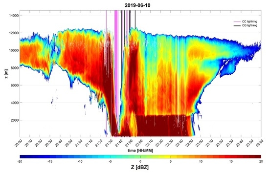
1. Introduction
Investigation of atmospheric electricity and lightning has started several hundred years ago and intense attention to processes of cloud electrification has been examined over the last several decades. However, our knowledge is still not complete because of our limited abilities to measure and observe processes, which occur in the atmosphere. It is supposed that the existence and development of electric field in the atmosphere is related to cosmic rays [1,2] and synergy of hydrometeors in clouds [3]. Currently, it is widely accepted that the main process leading to cloud electrification and lightning discharges is the process of riming electrification, often called the non-inductive charging [3,4,5,6]. In the non-inductive charging, it is assumed that the charging occurs mainly due to collisions of hydrometeors; between ice and graupel hydrometeors in particular [3,5].
Except for mathematical models, research data on electrification processes are available from laboratory experiments [7,8] and field campaigns carried out in thunderclouds (e.g., balloon experiments, aircraft data) [9,10,11,12,13] or they can be derived from satellite or radar observations [14,15,16,17,18,19]. Cloud radars represent an important data source for estimation of distribution of hydrometeors and for derivation of vertical air velocity. Thereby in thunderclouds, the cloud radars may provide necessary information for the charging mechanism by collisions of hydrometeors. In addition, measurements from polarimetric cloud radars can be used to indicate the electric field in cloud. Vonnegut [20] was the first, who described that ice crystals align within the electrostatic field in thunderstorms. Since that time, there were other studies suggesting it as well [21,22,23,24]. This alignment of highly asymmetric ice particles is assumed to be indicated by clearly higher values of depolarization [25,26,27,28].
In this paper, we study differences in distribution of hydrometeors and in values of Linear Depolarization Ratio (LDR) in thunderclouds in dependence on whether a lightning discharge was recorded in the vicinity of the radar site or not. Based on data from a vertically-oriented polarimetric cloud radar, we estimate 5 hydrometeor species and we compare the identified hydrometeor species together with LDR values with lightning observations recorded by EUCLID (European Cooperation for Lightning Detection) network.
The paper is organized as follows. After this introductory section, Section 2 provides the reader with description of the cloud radar and of algorithms, which we apply to derive vertical air velocity (AV) and to classify hydrometeor species (Hclass). This section also provides an overview of analyzed thunderstorms and describes methods of comparison between obtained or derived data from the cloud radar and recorded lightning discharges near the radar site. Section 3 displays results; it details a thunderstorm that occurred on 10 June 2019 from diverse perspectives and then it shows common characteristics and average vertical profiles of LDR of (all) analyzed thunderstorms. Section 4 discusses the obtained results, while Section 5 draws conclusions of this study.
2. Materials and Methods
2.1. Vertically-Oriented Cloud Radar
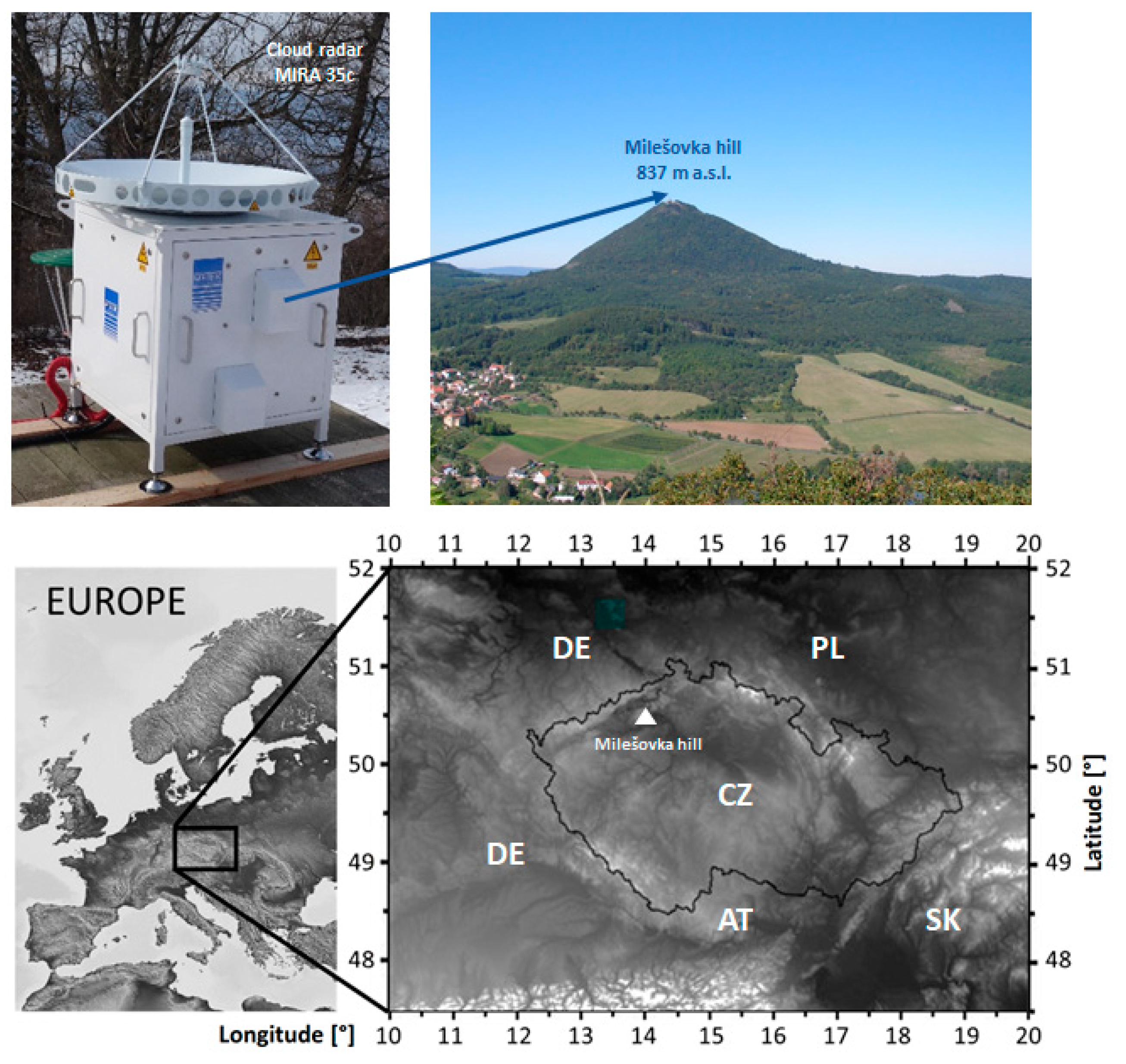
A vertically-oriented Ka-band cloud radar MIRA 35c manufactured by METEK Gmbh (http://metek.de/) was mounted at the top of Milešovka hill (837 m a. s. l.) at a meteorological observatory (Figure 1) in Central Europe (northwestern Czechia; 50°33′18″ N and 13°55′54″ E) in March 2018. The polarimetric cloud radar (i.e., cloud profiler) works at a frequency of 35 GHz. After calibration of the instrument, the radar began operating in June 2018. Table 1 provides the reader with the technical specifications of the radar.
The cloud radar is equipped with an Interactive Data Language (IDL) software enabling the basic processing and visualization of Doppler spectra (http://metek.de/product/mira-35c/). Doppler spectra are obtained after averaging 40 consecutive values and after estimation of noise floor. Values below the estimated noise floor are considered as NaN values (they have no signal). The IDL software calculates three moments of averaged Doppler spectra such as radar reflectivity (Z), Doppler vertical velocity (DV) and spectrum width (σ). Among derived quantities, one also obtains values of Signal-to-Noise Ratio (SNR) and values of Linear Depolarization Ratio (LDR). Approximately, the radar records are available every 2 s from 509 gates. Gates are denoted ig = 4, …, ig = 512 because the first three gates (ig = 1, ig = 2, and ig = 3), which are closest to the ground, are not processed. The distance between two consecutive gates is 28.8 m.
In this study, we use averaged noise-free Doppler spectra to estimate vertical air velocity (AV) and derive five hydrometeor species. The algorithm deriving AV as well as the algorithm classifying hydrometeors (Hclass) are described in Section 2.2 and Section 2.3.
2.2. Calculation of AV
The calculation of AV is crucial for classification of hydrometeor species (Hclass, Section 2.3) because the classification is mainly based on their terminal velocity (TV). The cloud radar measures composed velocity (DV) of TV and air velocity (AV), such as DV = TV + AV. When calculating AV, the AV is oriented towards the radar (downward) in accordance with basic processing of measured data by the IDL software used by the radar manufacturer. At the end of our calculation of AV, however, the AV orientation is reversed and we present all outputs of AV with upward orientation.
AV calculation is based on very small particles in Doppler spectra that are assumed to be so light that their TV is very close to zero, i.e., they are carried solely by air, and thus their velocity defines the AV. This is a common approach that was detailed by Kollias et al. [29], Gossard [30] and Shupe et al. [31], and conducted by, e.g., Zheng et al. [32] or Sokol et al. [33]. In this study, we innovated the algorithm used by Sokol et al. [33] to derive AV from variances caused by turbulence, wind shear, particle size distribution, and finite radar beam width.
We found that the original algorithm used for AV calculation, which performs de-aliasing of the Doppler spectra, can lead in some cases to significant and unrealistic temporal changes of AV, which then result in erroneous hydrometeor classification. That is why our new de-aliasing algorithm uses three methods of AV calculation, compares the result of each of them (AV1, AV2 and AV3) with the result of the two others and also compares the three calculated AV with the AV calculated for the previous cloud radar recording, i.e., 2 s back in time, approximately (AVL).
Any Doppler spectrum is stored for each gate in intervals beginning with a component ia and ending with a component ib, where ia corresponds to lower speed and ib to higher speed. The intervals, which are identified by the algorithm of the manufacturer of the cloud radar, represent continuous parts of a Doppler spectrum which are ordered from the lowest speeds. Note that for a gate, we can obtain multiple intervals. Components, which are not part of any determined interval, are considered to have zero amplitude. In this study, we consider not only the interval with the lowest magnitude of velocity corresponding to ia in the first interval (Sokol, Z. et al. [33]), but also the ia from the second interval.
We assume that measured values might be aliased. Therefore, in addition to recorded values Vori, we also consider Vori ± Vd values, where Vd = VNyquist + VNyquist (for VNyquist value see Table 1). We use parameters qtol = 3 and qmax1 = 5 in the following calculations of AV. The calculations of AV consist of steps provided below, which are performed for individual gates (ig) from the bottom (ig = 4) to the top (ig = 512) because AV is not affected by aliasing in the lowest gates as updrafts cannot be that strong (>VNyquist) near the ground. We calculate AV1, AV2, AV3 and AVL and assign the resulting AV to the value (i.e., among AV1, AV2, AV3 and AVL) that best corresponds to conditions described in the next paragraph. In the de-aliasing algorithm, we also use a reference value Vref, which is define in steps 7, 8 and 9 in the procedure described below.
The procedure of AV calculation consists of following steps:
- For an ig (ig = 4 at first), we define de-aliasing function (DAL) calculating velocity Vcor using original and reference velocities Vori and Vref, respectively:where Vcor corresponds to one of the values (Vori, Vori + Vd or Vori - Vd) that is closest to the value Vref.Vcor = DAL(Vori, Vref),
- AV1 is calculated in the same way as by Sokol et al. [33], i.e., we consider only those components of Doppler spectra whose amplitude is at least 0.1% of the maximum Doppler spectra amplitude.
- AV2 is calculated in the same way as in point 2 but without the mentioned condition concerning the maximum Doppler spectra amplitude.
- In addition to the (first) interval corresponding to the lowest speed, we also consider the (second) interval corresponding to the second lowest speed. We determine AV3 as the most left point of the second interval. The reason is that it can happen that the first interval containing the lowest speed is very narrow and far from the second interval. A closer comparison commonly shows that the first interval is likely an unremoved noise since its values are usually inconsistent with values in a gate below and a gate above and these values are also inconsistent with the values recorded in previous measurements. In such a case, it is evident that the second interval should also be considered in AV calculation (AV3).
- We take into account AV calculated for the same gate but in the previous recording (≈2 s prior to the investigated recording) and we denote the resulting value AVL.
- If AV(ig − 1) is available, then we calculate AV(ig) using the following:AV1cor(ig) = DAL(AV1(ig), AV(ig − 1))AV2cor(ig) = DAL(AV2(ig), AV(ig − 1))AV3cor(ig) = DAL(AV3(ig), AV(ig − 1))If |AV2cor(ig) - AV(ig − 1)| < qtol, then AV(ig) = AV2cor(ig), stopIf |AV1cor(ig) - AV(ig − 1)|, then AV(ig) = AV1cor(ig), stopIf |AV3cor(ig) - AV(ig − 1)|, then AV(ig) = AV3cor(ig), stop
- If all the above given conditions (no. 6) are fulfilled, then AV(ig) is assigned according to the nearest value among AV1cor(ig), AV2cor(ig) and AV3cor(ig) to Vref = AV(ig − 1) if AV(ig − 1) is available.
- If AV(ig − 1) is not available but AVL(ig) is available, then:Vref = AVL(ig) and AV(ig) = DAL(AV2(ig), Vref(ig)).
- If AVL(ig) is not available, which usually does not happen, then AV(ig) from more past recordings is used as Vref.
- AV(ig = 4) is calculated using no. 7 and if AV(ig = 4) > qmax1, then AV(ig = 4) is set to AV(ig4) − Vd, because we do not allow large positive values of AV.
- We repeat the procedure from no. 1 to no. 9 for the next gate, i.e., one gate higher (ig = ig + 1).
- The procedure finishes at the highest gate (ig = 512) or at the (highest) gate, where we still recognize discrete intervals of Doppler spectra in the radar data.
It should be noted that the applied procedure determining AV based on very small particles (tracers) is limited by how well very small particles are identified in the Doppler spectra. It may happen, especially in the case of heavy rain, that smallest particles with negligible terminal velocity are not detected anymore due to extinction or that in the radar volume of some gates, there are only larger droplets likely due to size sorting. This is related to spots in thunderclouds with high LWC, which make the larger droplets arrive earlier to lower gates. However, our experience suggests that these are very rare cases and their effect is marginal.
Calculation of AV precedes the classification of hydrometeor species (Hclass) because AV cannot be neglected in summer thunderstorms that are under investigation in this paper. Thunderstorms are a convective phenomenon for which (strong) updrafts and downdrafts are typical.
2.3. Clasiffication of Hydrometeor Species—Hclass
Hclass performed in this paper is similar to Sokol et al. [33] and stands on the idea that the TV of diverse hydrometeor species differs. It is natural that the existence of a hydrometeor species depends on ambient air temperature and its shape can be identified by LDR (e.g., shape of ice crystals differs from that of rain). In this paper, we define five hydrometeor species; cloud water (i.e., cloud droplets), rain, graupel, hail, and ice and snow particles together. We merged ice and snow particles into one group following the recommendations provided by Sokol et al. [33], where the algorithm was not able to efficiently distinguish ice particles from snow.
Terminal velocity range of the 5 hydrometeor species between minimum terminal velocity (TVmin) and maximum terminal velocity (TVmax) is provided in Table 2. Terminal velocity ranges of hydrometeor species do not overlap and stem from values provided in COSMO numerical weather prediction model. We use these values as “standard” values for hydrometeors whenever we make model simulations over Czechia (e.g., Sokol et al. [34]). The actual TV of a target for any discrete interval of Doppler spectra corresponds to the result of subtraction of AV from DV for a given peak of the Doppler spectra.
We define the ambient air temperature (T [°C]), which influences the presence of hydrometeor species, from ERA5 reanalyses (www.ecmwf.int). Specifically, we take temperature profiles of a grid point closest to the Milešovka observatory. ERA5 reanalyses provide us with hourly data at a horizontal resolution of 0.25° (geographical latitude) × 0.25° (geographical longitude). The use of ERA5 reanalyses differs from Sokol et al. [33], which used temperature profiles based on sounding measurements from Praha/Libuš station situated 60 km southeast from the Milešovka observatory. These sounding data are not only distant from the Milešovka observatory, which is a problem especially when investigating thunderstorms, but they are also available only at 00, 06 and 12 UTC. On the other hand, ERA5 reanalyses provide us with vertical profiles at a higher (i.e., hourly) temporal resolution and from a location much closer to the radar site (12 km). Thus, we consider ERA5 reanalyses more suitable for this study. On the other hand, we are aware that the used temperature profiles are not accurate because the ERA5 data have a low resolution to describe temperature profiles in convective storms that differ from those of the surrounding air.
Similar to Sokol et al. [33], we use 0 °C as a temperature threshold in the Hclass algorithm and as in Sokol et al. [33], if T > 0 °C, then the Hclass provides cloud water, rain, graupel or hail. However, if T ≤ 0 °C, we determine the existence of supercooled water in the higher atmospheric (i.e., tropospheric) layers differently than Sokol et al. [33]. Sokol et al. [33] used a fixed threshold of -20 °C below which the supercooled water could not exist although in the case of convective storms, it can happen that the supercooled water is observed at much lower temperatures (even at −50 °C in some cases) due to strong updrafts and lack of time to freeze. Therefore, we modified the Hclass provided by Sokol et al. [33] and set that the supercooled cloud water can be found from 0 °C up to −40 °C (instead of previous −20 °C), which corresponds to generally accepted temperature range for the existence of supercooled water in mid-latitude summer thunderstorms. We define the existence of supercooled cloud water within 0 to −40 °C only if a condition of AV is met: (i) AV > 1 m/s if T is between 0 °C and −20 °C or (ii) AV(T) =1 − (T + 20)/5 if T is between −20 °C and −40 °C. The threshold for AV and relationships determining supercooled cloud water were obtained empirically based on subjective evaluation of their performance at various thunderstorms recorded by the cloud radar.
A limitation of our Hclass is that we did not have the means to objectively verify its results. Since any Hclass depends on selected terminal velocity range of individual hydrometeors and real measurements show ambiguity in the terminal velocity ranges, any change in terms of terminal velocity range of any hydrometeor species will affect the results of all Hclasses. This is the key source of uncertainty of Hclasses in general. Moreover, while fixing the values of given parameters (e.g., terminal velocity range), it is almost impossible to avoid subjectivity. Thus, we tested several values of parameters, compared obtained results and fixed the parameters to values that provided results closest to reality based on our experience and/or literature.
2.4. Analysed Data: Thunderstorms of 2018 and 2019
In this study, we used data of the cloud radar situated at the Milešovka observatory (Figure 1) such as Z, LDR, derived AV (Section 2.2) and classified hydrometeor species (Section 2.3) during days with lightning registered up to 20 km from the Milešovka observatory by the EUCLID network. The data covered a period from June 2018 to September 2019. The dataset consisted of 38 days of thunderstorms (Table 3). Continuous data records lasted at least 2 h and more than one thunderstorm could have occurred during a single (analyzed) day.
For the dataset of 38 days of thunderstorms (Table 3), we dispose of ground-based observations of lightning discharges by EUCLID network [35]. We obtained the data from Blitz Informationsdienst von Siemens (BLIDS) [36], which provides it to EUCLID network, for the whole territory of Czechia and its neighborhood. BLIDS uses the time of arrival (TOA) principle to locate lightning discharges. TOA principle is based on assumption that the electromagnetic field induced by a lightning discharge propagates at the speed of light from its origin in all directions. Individual receivers record TOA and the difference in TOA among receivers defines the location of the discharge.
The lightning data include information on geographical coordinates of the discharge (in WGS84), time of the discharge [ms], peak current [kA], polarity of the discharge, type of the discharge (Cloud-to-Ground CG and Cloud-to-Cloud CC), and on quality of data (binary information). The spatial accuracy of the lightning dataset was 0.6 km (median) at a confidence level of 95%, while the lightning detection efficiency was about 100% [37]. All the data used in this study were of good quality according to the binary information in the lightning dataset.
In addition, we obtained weather radar reflectivity factor data at various Constant Altitude Plan Position Indicator (CAPPI) levels for the 38 days of thunderstorms (Table 3) from the Czech radar network (CZRAD; Sokol et al. [38]) operated by the Czech Hydrometeorological Institute. CZRAD network consists of two C-band weather radars recording measurements every 5 min at a horizontal resolution of 1 km. The closest radar is located 100 km southward from the Milešovka observatory. Main product of the two C-band weather radars is the radar-derived rain rate (R [mm/h]), which we calculate using the Z–R relationship, such as Z=200R1.6, where Z is the radar reflectivity factor [mm6/m3] [39]. Furthermore, we had synoptic data from the Milešovka observatory at our disposal, and in this study, we used rain gauge measurements with a temporal resolution of 1 min.
2.5. Methods of Comparison between Cloud Radar Data and Lightning Data
The comparison of cloud radar data with lightning data is not straightforward due to differences in their location. The cloud radar is a profiler, i.e., it registers a vertical profile from a particular location on the ground, whereas lightning data can be registered anywhere. Thus, in this study, we reduced the lightning dataset to lightning discharges that were located within a circular area around the Milešovka observatory, where the Milešovka observatory was situated in its centre. We considered several circular areas (with a radius of 1, 2, 3, 5, 7, 10, and 20 km) around the Milešovka observatory.
We decided to divide storms above the radar into storms with lightning (denoted “near lightning”, NL) and those without lightning (denoted “far lightning”, FL). After several testing, we selected 1 km as the radius defining NL because we believe that this is the distance, which describes the condition of a cloud above the Milešovka observatory, when the development of lightning (i.e., electrification) is taking place or will soon take place over the Milešovka observatory (or its nearest vicinity). Contrary, the FL (lightning registered at a distance of 10-20 km from the observatory) represent the condition of a cloud above the Milešovka observatory, when no discharges were recorded in its direct vicinity. In Section 3, we depict results for NL as compared to FL.
Another issue in comparing cloud radar data with lightning data is the difference in their temporal resolution. Cloud radar data are recorded every 2 s approximately, while lightning data are registered at a temporal resolution in the order of ms. However, this is not of high importance since based on our experience the temporal variability of radar measurements is not very high, even in thunderstorms.
Being aware of the difference in temporal resolutions of radar and lightning data, we still decided to consider cloud radar data registered just before and just after the time of any lightning discharge; i.e., we considered two consecutive cloud radar recordings (distant by 2 s) that we coupled with a lightning discharge. This way, we compared cloud radar data (vertical profiles of Hclass, AV and LDR) with lightning data in circular areas around the Milešovka observatory (NL vs. FL) during the 38 days of thunderstorms (Table 3). Note that there were 990 lightning discharges observed up to 1 km from the Milešovka observatory during the 38 days of thunderstorms and 171,754 FL discharges.
3. Results
This section is divided into two parts. The first part describes a particular thunderstorm that occurred on 10 June 2019. We selected this thunderstorm because on that date, the observer recorded a thunder less than 1 s after he saw the lightning flash at the Milešovka observatory. According to geographical coordinates in EUCLID data, the lightning discharge occurred at a distance of only 65 m from the observatory. This lightning discharge was the second closest in our dataset; on 1 June 2018, there was a lightning detected directly at the observatory, which hit the observatory according to the book of records written by observers. Nevertheless, we do not detail this thunderstorm (on 1 June 2018) in this study since Sokol et al. [33] already studied it in detail.
Contrary to the first part of this section, which is dedicated to one particular thunderstorm, the second part of this section presents common characteristics, including LDR, that were typical throughout all thunderstorms that occurred in the 38 days in the dataset (Table 3). It presents results from the comparison of cloud radar data with lightning data in dependence on the distance of lightning discharge to the Milešovka observatory (i.e., NL vs. FL).
3.1. Thunderstorm on 10 June 2019
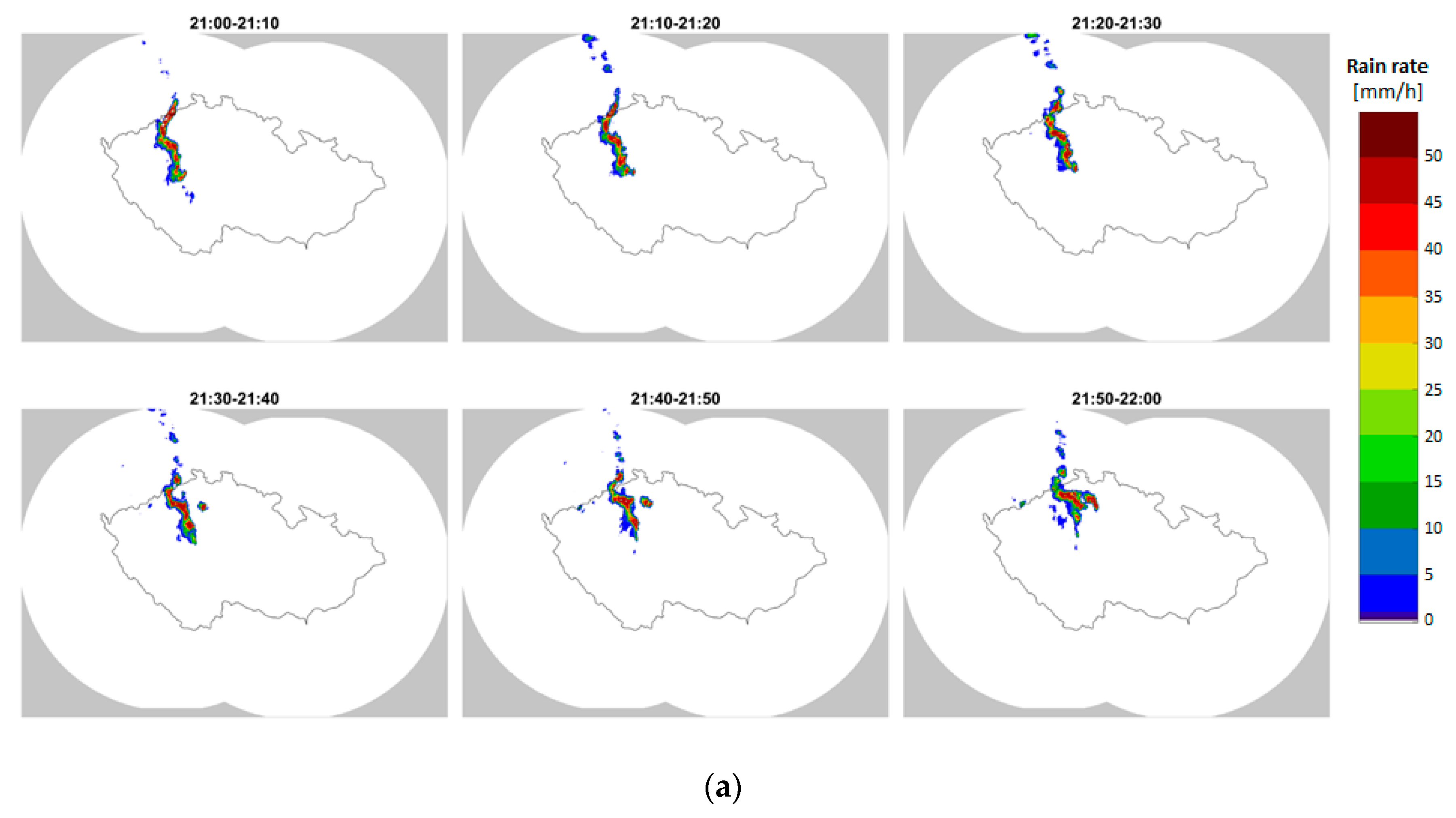
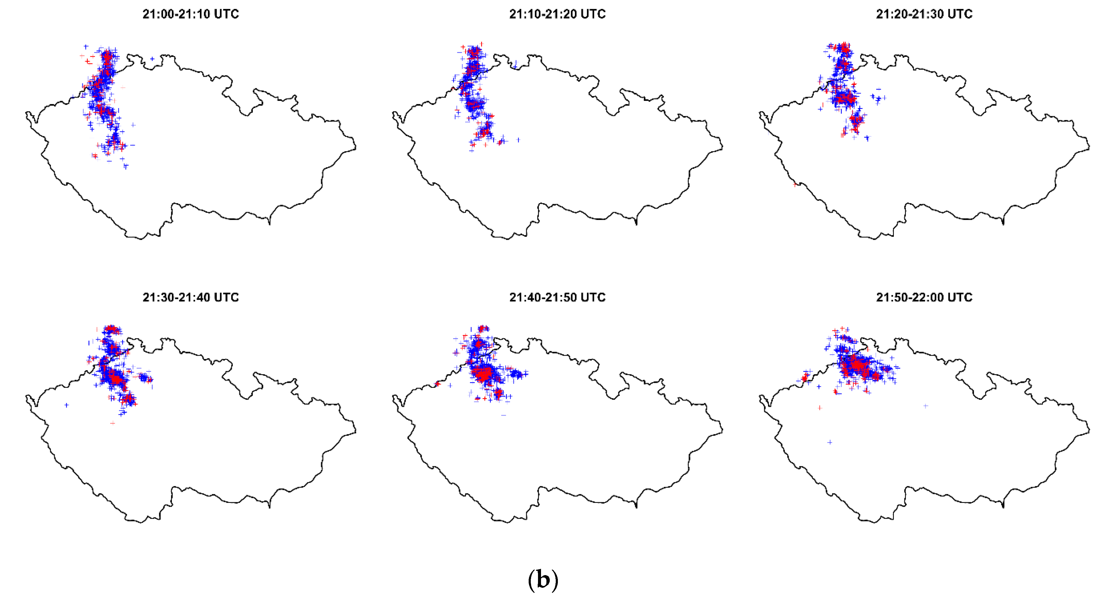
Figure 2 shows the temporal evolution of rain rates (as derived from C-band weather radar data, Figure 2a) and lightning discharges (Figure 2b) during one hour of the thunderstorm on 10 June 2019, when most lightning activity was observed close to the Milešovka hill. The temporal evolution is displayed with a time step of 10 min. Based on rain rates (Figure 2a), it is clearly visible that the thunderstorm was severe, at least within the central European context.
Figure 2 also shows that the lightning discharges occurred (horizontally) not only within the precipitation areas but also outside of the precipitation cores; i.e., they may have originated in non-precipitating parts of the thundercloud as well. As the system moved in time towards east-northeast, CC flashes had a tendency to precede CG flashes, while lightning flashes (CC + CG together) tended to occur not only during the period of intense rainfall, but also prior to intense rainfall. This has been mentioned in other works as well, e.g., [40].
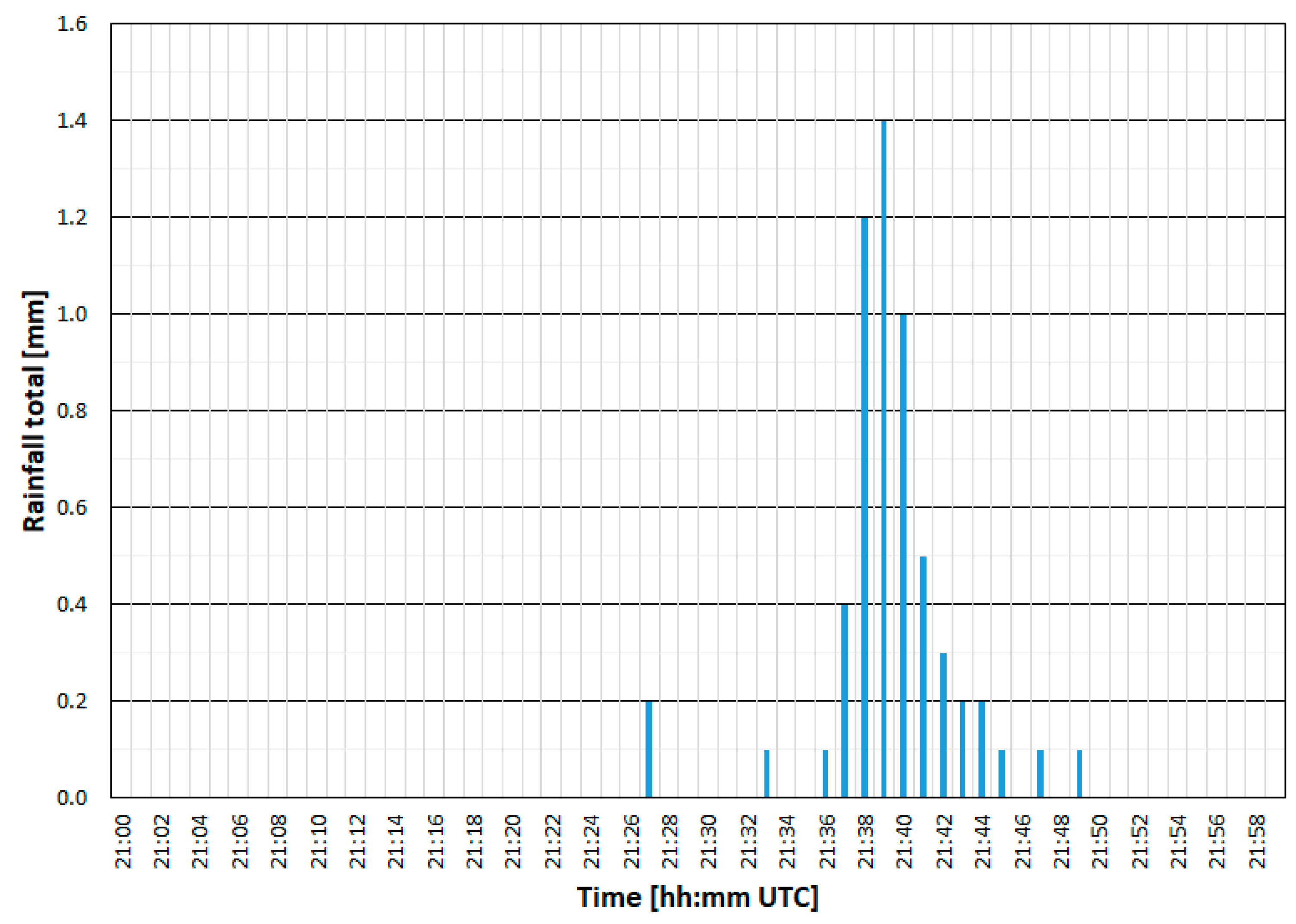
Figure 3 depicts precipitation totals with a time step of 1 min, as registered by a rain gauge with a resolution of 0.1 mm at the Milešovka observatory between 21 and 22 h UTC on 10 June 2019. Note that rain rates (i.e., precipitation intensities, Figure 2a) cannot be directly compared with recorded precipitation totals (Figure 3) as they do not represent the same information. Figure 3 shows that the highest 1-min precipitation total occurred between 21:39 and 21:40, while the closest lightning was recorded at 21:37 and 50.341 s. This confirms that lightning flashes may occur prior to heavy rain. Here, we note that measured precipitation totals by the rain gauge might be underestimated. The reason is that at the top of Milešovka hill, strong winds frequently appear during storms, which may result in an underestimation of rainfall totals due to the blowing away of the precipitation from the surface of the rain gauge.
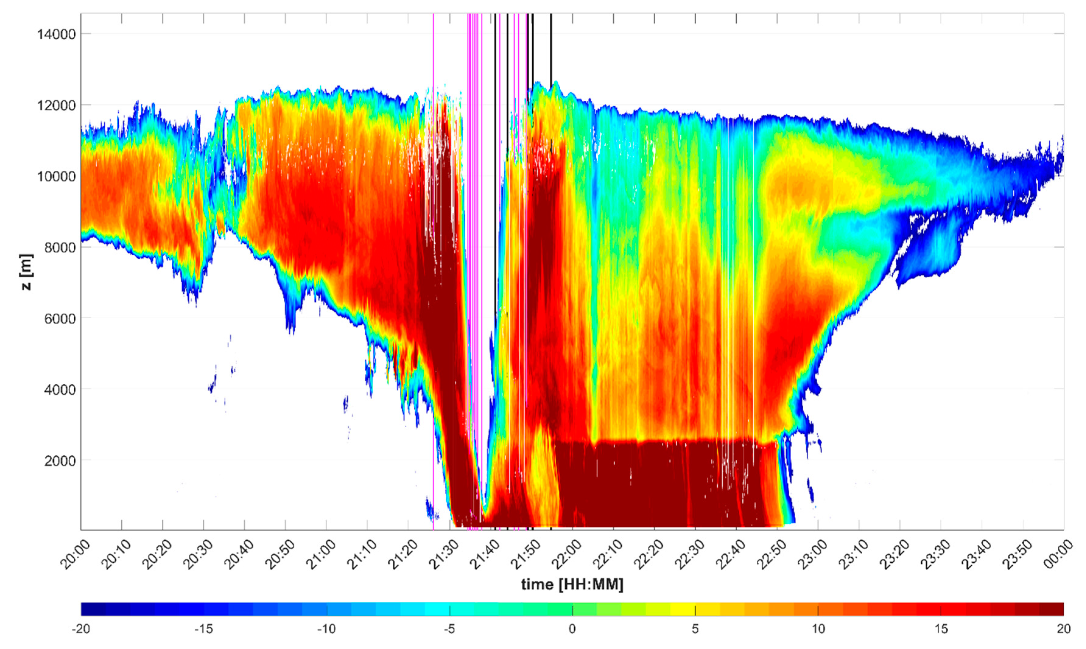
Concerning data of the cloud radar, Figure 4 displays radar reflectivity together with NL (i.e., lightning discharges that occurred not farther than 1 km from the Milešovka observatory). It is obvious from the figure that NL were related to high reflectivity values, although high reflectivity values were also typical for the melting layer and below (i.e., below 2.5 km approximately).
It is worthy of note that between 21:30 and 21:40 approximately, there was a sudden decrease in the vertical span of the thundercloud, according to the cloud radar data (Figure 4). This is the time when most of rainfall was registered at the Milešovka observatory (Figure 3). This is probably caused by the fact that the received signal in the lowest gates was too strong due to heavy rain that the radar was unable to capture signal from higher gates.
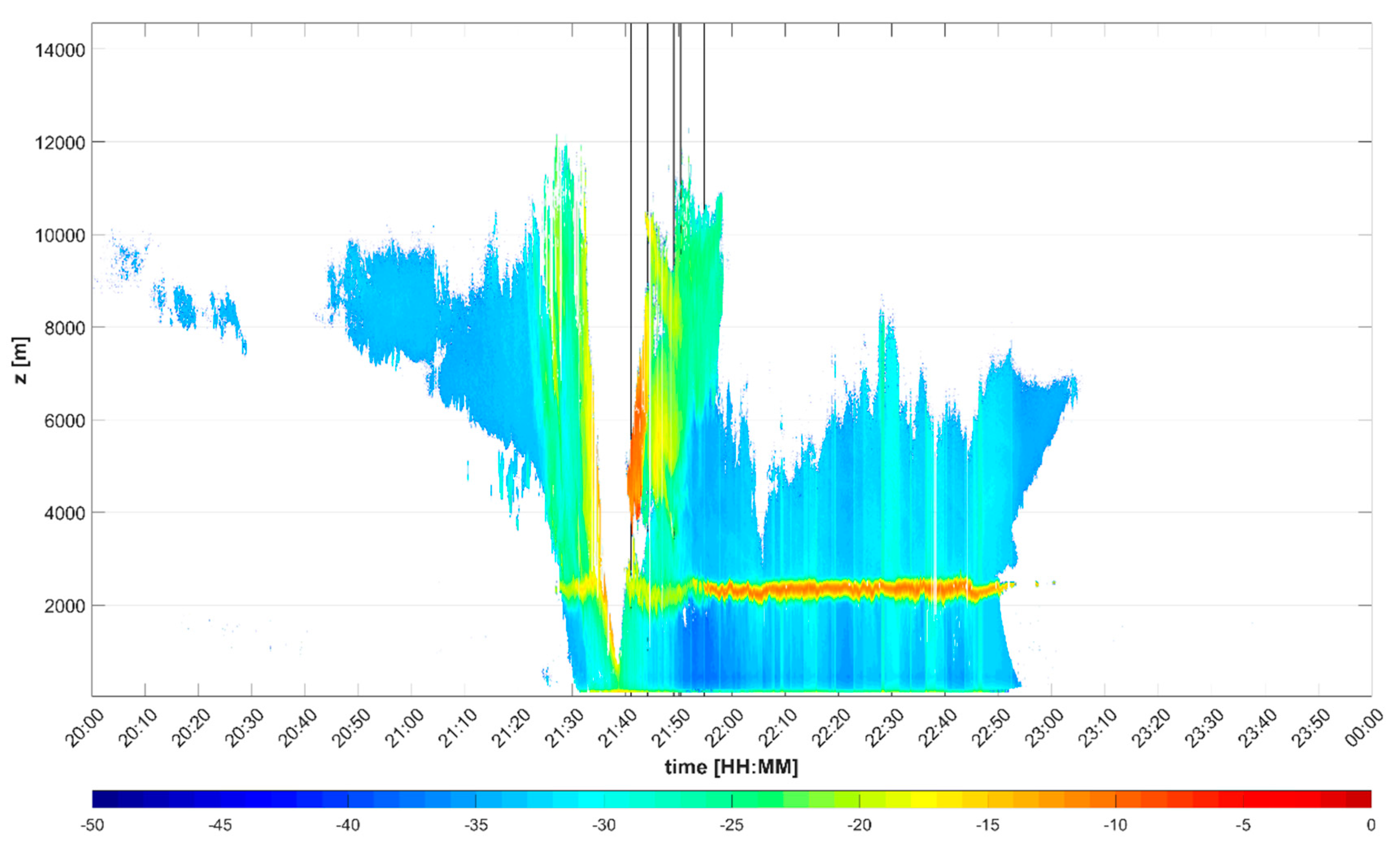
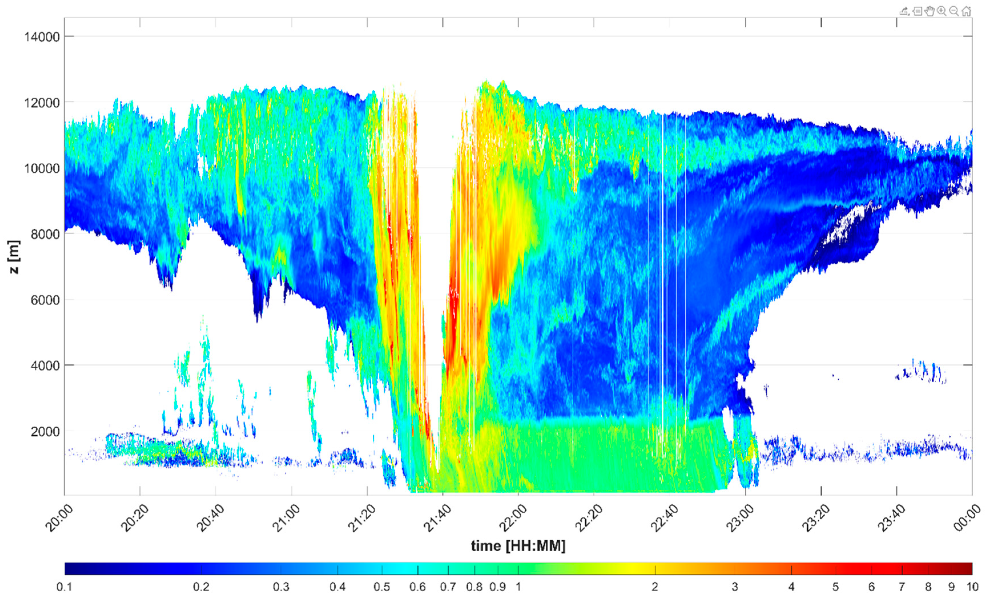
Furthermore, it is interesting to check the temporal evolution of LDR values during the thunderstorm (Figure 5) that were not corrected using the integrated cross-polarization ratios [41]. In Figure 5, high values of LDR clearly show that the melting layer was around 2500 m above ground in the thunderstorm. Another zone of high LDR values is visible from 21:30 to 21:50 at higher altitudes, which is the time interval of intense rainfall (Figure 3) and lightning activity near the radar site (Figure 4). Contrary to very high LDR values in the melting layer, which are commonly associated with melting snow flakes, very high LDR values at higher altitudes, such as 4-7 km, can correspond to non-spherical shape of graupel and/or hail or to aligned ice crystals due to a strong electric field if the crystals are not aligned along with the co-channel, instead they are oriented at angle close to 45° with both the co- and cross-channels [25,42,43]. It is worthy of note that the elevation around 4-7 km, where we observed increased LDR, is also considered as the elevation where the main negatively charged area appears [40]. We discuss this finding further below.
It should be noted that the LDR data are not available at all gates where we obtained radar reflectivity factor data (for example, after 21:50). This is the consequence of the attenuation of the signal received in the plane perpendicular to the transmission plane.
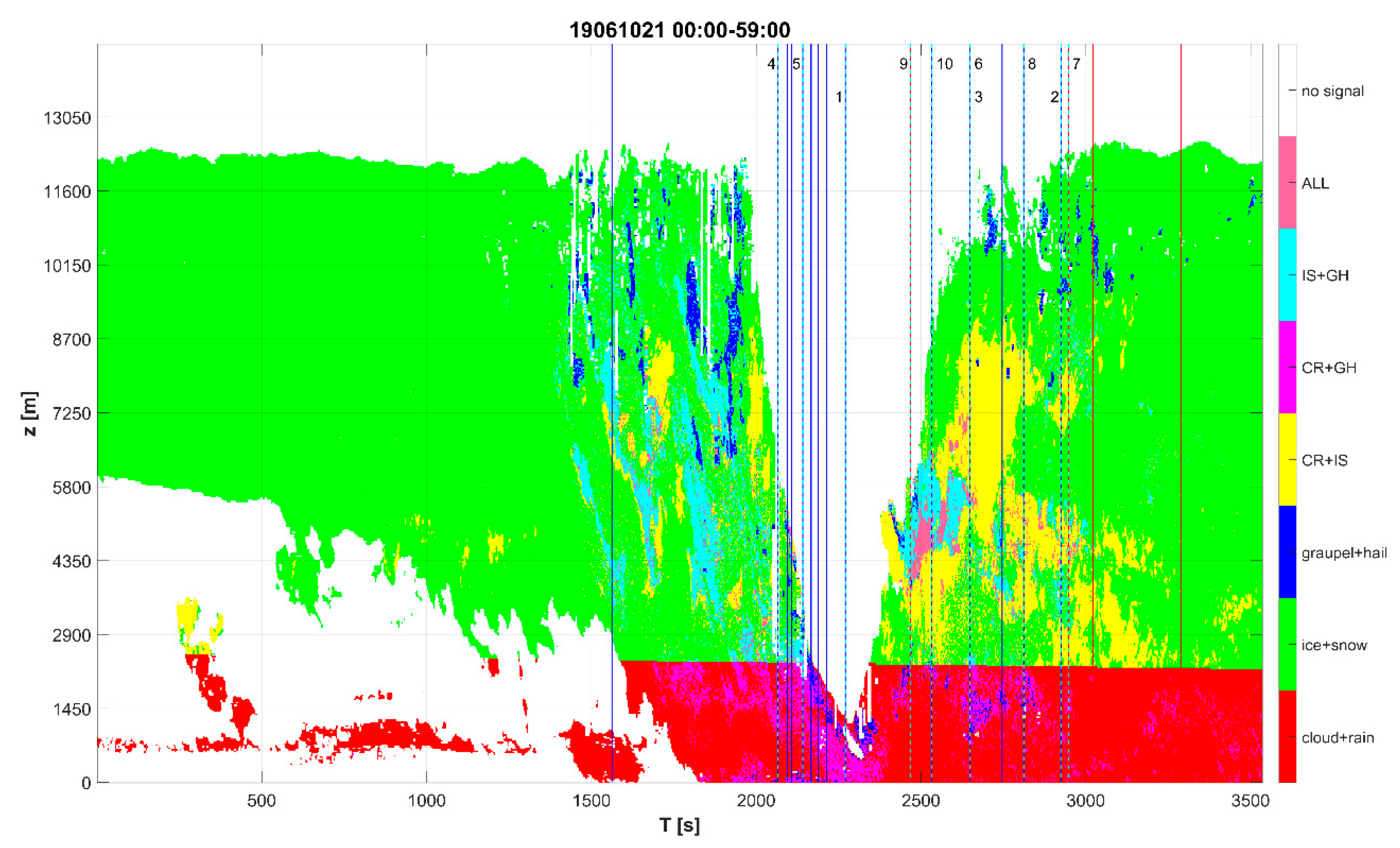
Figure 6 shows the evolution of hydrometeor distribution (resulting from Hclass, Section 2.3) on 10 June 2019 from 21:00 to 21:59 UTC. Clearly, the lack of data in the vertical profiles between approximately 21:30 and 21:40 makes the interpretation of the obtained results difficult, especially because many NL discharges occurred at that time. Nevertheless, the majority of the ten closest discharges (Figure 6) occurred after 21:40, when we had data again, covering almost all the troposphere.
The results of Hclass indicate that the highest LDR values at the elevation from 4 to 7 km (Figure 5) correspond to a mixture of several hydrometeor species with a predominance of ice and snow particles and graupel. These are the species which play major roles in the process of cloud electrification by collisions of hydrometeors according to currently accepted theories [44]. The mixture of many hydrometeor species is also evident during very close lightning activity (between 2400 s and almost 3000 s in Figure 6).
The electrification process by collisions of hydrometeors at an elevation of 4–7 km is also supported by Figure 7, which presents values of the Doppler spectrum width (σ). High values of σ, i.e., large variability of vertical velocities, just after 21:40 confirm the coexistence of various hydrometeors and support the existence of collisions of hydrometeors (light species collide with heavier species having larger terminal velocity). The obtained results of high LDR and sigma values together with the presence of diverse hydrometeor species may bring us to the conclusion that around 21:40, collisions of hydrometeors caused a strong electrification of the thundercloud near the radar site.
3.2. Common Characteristics of Analyzed Thunderstorms
This subsection focuses on results related tall thunderstorms in the dataset (Table 3). It shows their common (different) features and compares them with recent knowledge on lightning processes. Our intention was to compare NL with FL, when clouds were present above the observatory. Therefore, in the statistical evaluation, we used data from only those gates, where Hclass identified at least one hydrometeor species.
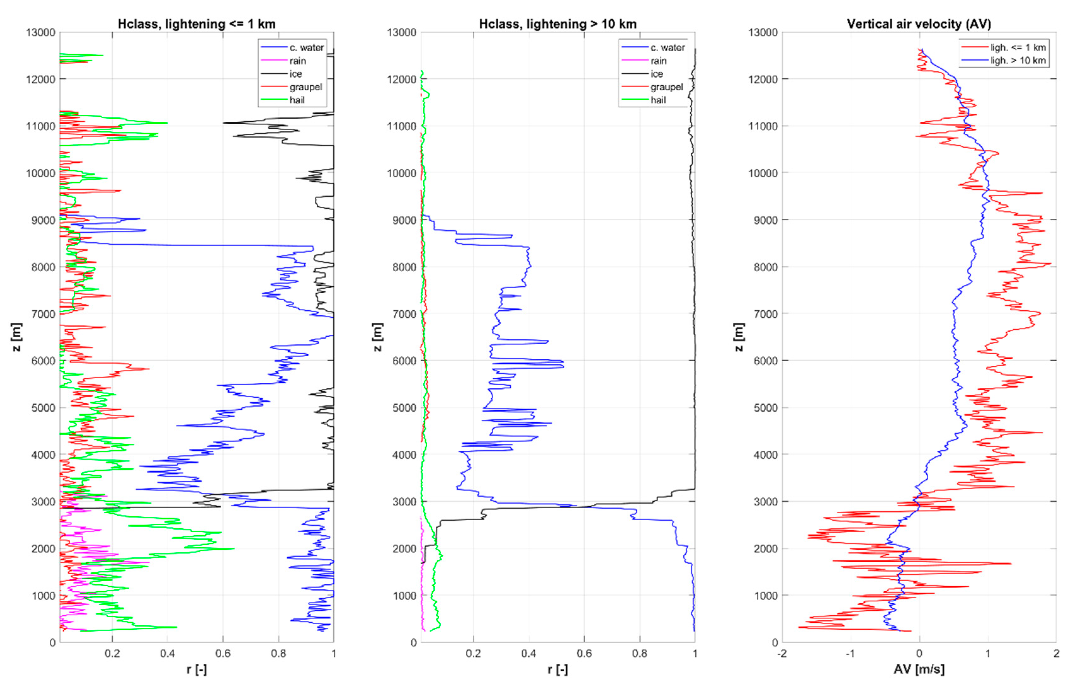
Figure 8 summarizes the results throughout the analyzed thunderstorms at the Milešovka observatory. It depicts radar-derived quantities for NL discharges compared to that for FL discharges. It clearly shows that on average, hail, rain and graupel occurred in lower gates more frequently during NL as compared to FL. For FL, rain and graupel were almost not detected at all. For NL, hail concentration was higher at an elevation of 2000 to 2500 m above ground. This is the level which roughly corresponds to the melting layer (Figure 4). Rain concentration was higher at lower elevations, at 1800 m approximately. Thereby, it can be suggested that the closer the lightning, the higher the concentration of rain and hail. This agrees with our previous results based on 10 thunderstorms [45].
In addition, Figure 8 displays the results of AV for NL vs. FL. It shows that in the case of NL, the downward motion of the air substantially prevails at lower altitudes; from the ground to 1000 m and from 2000 to 3000 m. The layer between 1000 and 2000 m above ground is characterized by fluctuations in AV, which can be related to an interchange of up- and downdrafts. Updrafts mostly dominate the elevation from 3000 m upwards. Slow updrafts are typical for very upper vertical levels (above 9500 m).
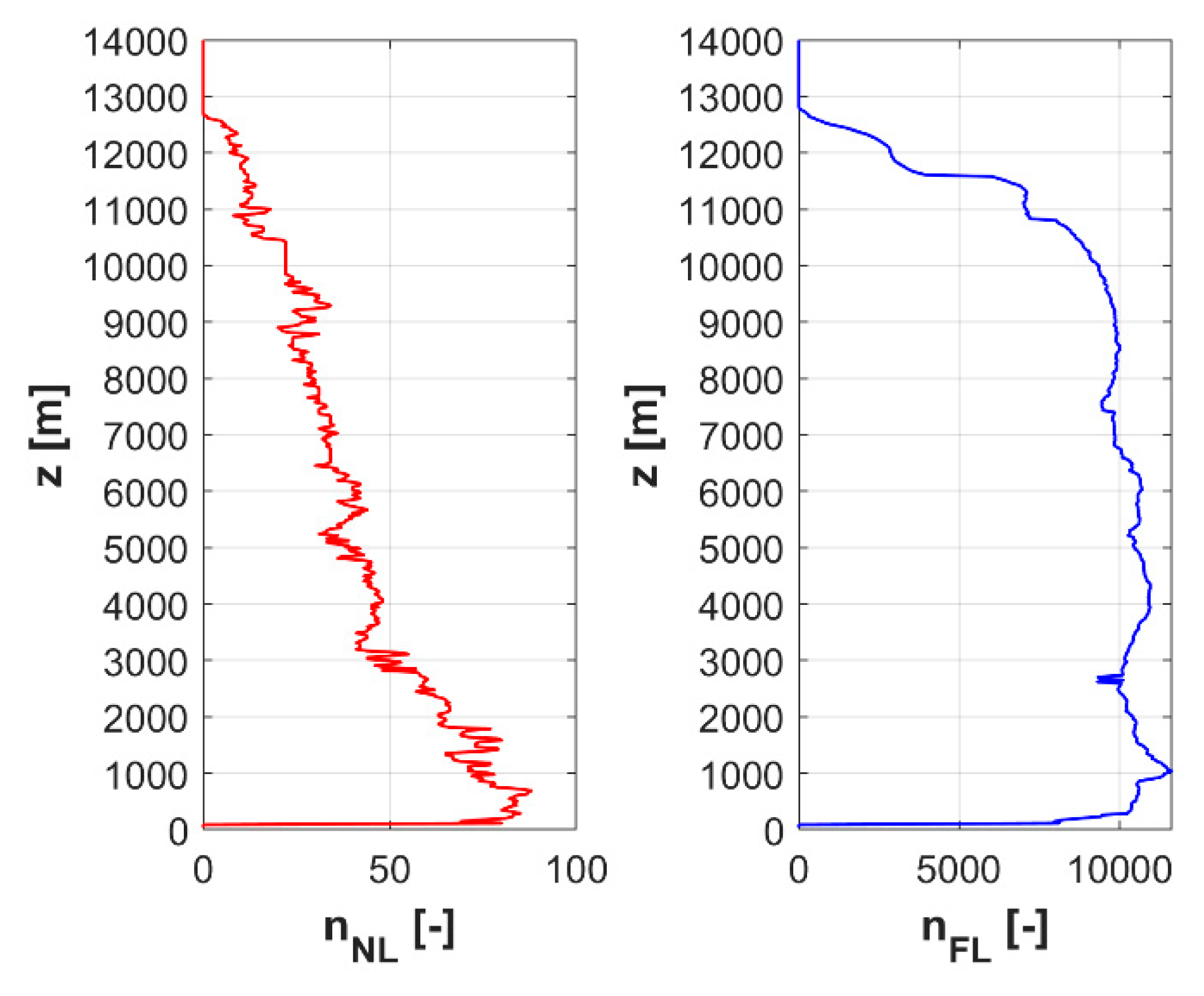
Overall, AV seems to be quite low, which is caused by averaging. The variability in AV among gates seems high for NL. This is caused by much lower number of NL discharges (990) as compared to FL discharges (171,754), as shown in Figure 9. Concerning FL, AV does not fluctuate much on average between neighboring gates, which is due to large number of processed data. Figure 8 also shows that for FL, downward motion prevails from the ground up to 3000 m, while upward motion dominates the layers above 3000 m on average.
Taking into account the distance of the lightning from the observatory, we do not know whether the radar measurements took place in the frontal or back side of the thunderstorms or on their lateral sides. The placement within the thunderstorm may lead to diverse directions and values of AV, which can be confirmed by high variability of AV (not depicted). In addition to the uncertainty regarding the localization of measurements with respect to the movement and development of thunderstorms, it should be emphasized that we present results and quantities that are derived indirectly (i.e., not directly measured). Therefore, the results cannot be explicitly verified. However, we can state that the obtained results are in accordance with the general knowledge about thunderstorms. Therefore, we believe that the technique used to calculate the vertical air velocity and to classify hydrometeors give realistic results.
3.3. LDR during Analyzed Thunderstorms
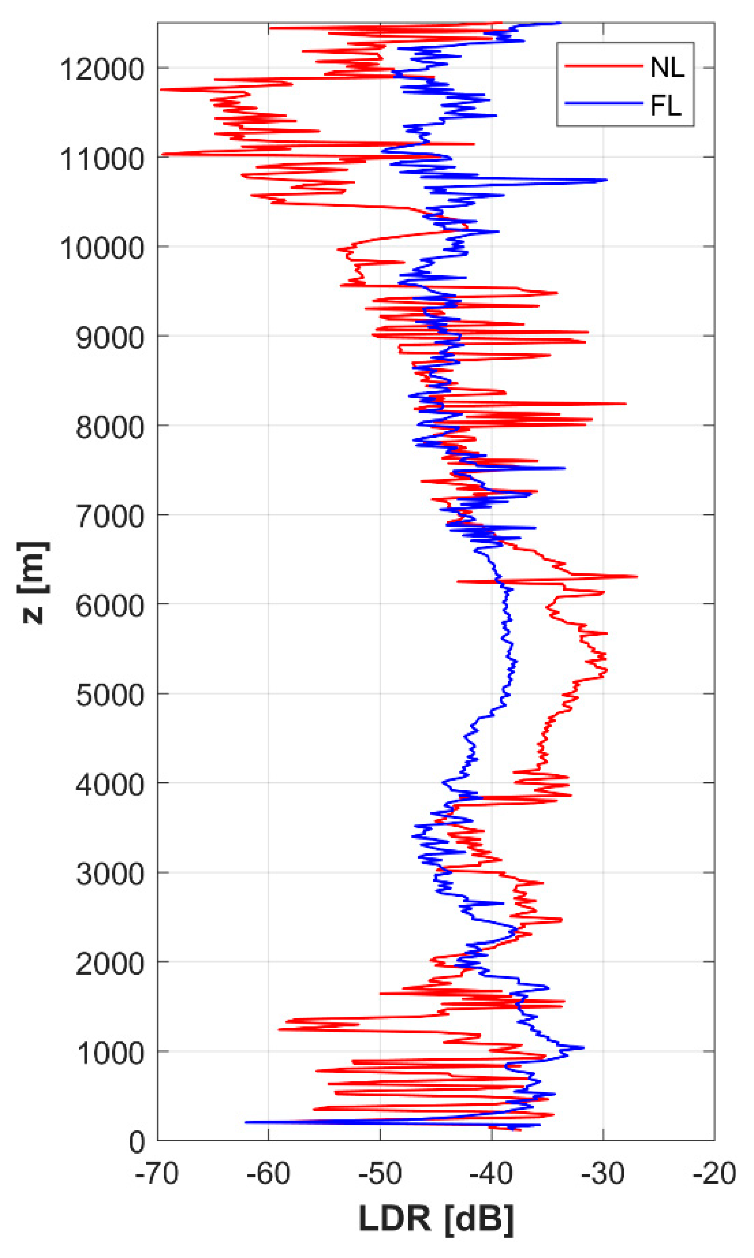
Averages of LDR are depicted in Figure 10 for NL, as compared to FL. For both NL and FL, the melting layer is not pronounced in LDR averages; there is no obvious increase in LDR averages in lowest gates. This is very likely related to the fact that the height of the melting layer depends on current atmospheric conditions, which change from one thunderstorm to another and might also change during one particular thunderstorm. As a consequence, the height of the melting layer becomes smooth in averaging, making it imperceptible in the figure.
The character of the curves in Figure 10 (their oscillation) is influenced by the number of averaged cases (Figure 9). This is especially true for the red curve representing NL discharges. The isolated maxima of LDR averages are probably random. However, Figure 10 clearly depicts that at an elevation of 4 to 6.5 km approximately, there are large LDR averages, which show little oscillations for NL, thus they do not correspond to random processes. These averages are much larger than the LDR averages for FL. As in Section 3.1, we attribute it to electrification by collisions and alignment of ice crystals.
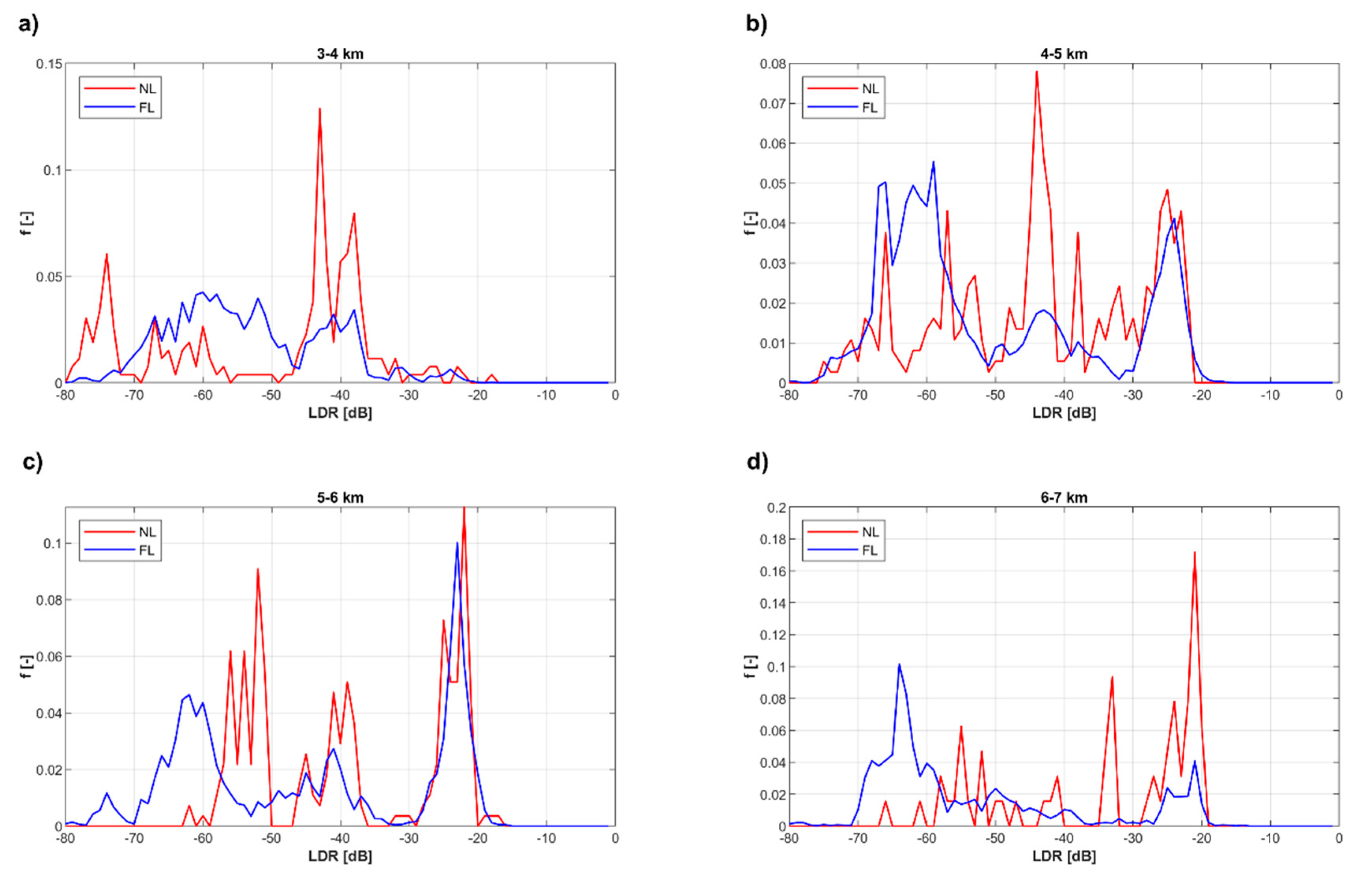
To better assign the cause of increased LDR averages in the middle troposphere, Figure 11 shows 1 km layers of frequency of LDR in profiles with similar distribution of graupel and hail (i.e., rounded hydrometeors). Because concentrations of graupel and hail are similar in both NL and FL (ice or snow being present almost everywhere in these 1 km layers, Figure 8), it is obvious that there had to be another process that made the higher LDR more frequent in the case of NL as compared to FL. We suggest that the additional process could be the alignment of ice crystals observed by other researchers, e.g., by Melnikov et al. [25]. However, we are aware that this hypothesis cannot be exactly verified.
At an elevation between 8 and 9 km, significantly higher averages of LDR for NL, as compared to FL, could be rather random because of high oscillations of that for NL. On the other hand, the high oscillations of LDR averages for NL can also be related to the orientation of aligned ice crystals in an electrified field. LDR can increase if the particles align at an angle close to 45° from both the co- and cross-channels, while it can decrease if the particles align along with the co-channel (LDR reaches large negative values). Thus, the LDR of non-spherical targets, such as ice crystals, can have strongly different values (large and small) depending on the azimuth direction to the channels. Therefore, the variability of LDR may be increased in the case of NL.
The results also suggest that the clouds producing lightning in the vicinity (NL) are vertically massive and higher than clouds producing FL, at least in our dataset.
4. Discussion
The method we chose, to distinguish between NL and FL, was based on the distance of observed lightning from the radar site. The results showed that the method can be applicable in general, however, it would be better if we could also identify in which part of the storm the vertical radar measurements are taken. We plan to focus on an analysis of the possibility to identify the position of radar within storms in future. Specifically, our aim is to study whether the radar is located on the frontal or back side of a storm or on its lateral sides. Such an analysis, however, needs a wider dataset of thunderstorms registered close to the radar, which we expect to obtain in future.
At present, the amount of data during two years of radar operation that meet the condition for NL is not sufficient to allow us to divide data into further subsets, which is necessary for the identification of where—in the thunderstorm—the radar is located. The division of the current dataset into further subsets would not lead to sufficiently robust results. Moreover, determining the position of the radar within a thunderstorm is not trivial and needs thorough investigations.
The distribution of data and the method of processing (averaging) inevitably led to a smoothing of AV. This smoothing (averaging) of vertical velocity resulted in low values of AV, since the dataset comprised both positive and negative velocities, which, after averaging, became naturally low. Nevertheless, regardless of AV smoothing, the profiles of mean AV for NL as compared to that for FL qualitatively correspond to our knowledge. During the mature state of a thunderstorm, (strong) positive as well as negative vertical velocities are supposed to be observed.
The applied technique for the recognition of hydrometeors (Hclass) provides meaningful results, although, of course, we cannot perform its exact verification. However, the structure of hydrometeors seems right during the maximum activity of the thunderstorm on 10 June 2019 (around 21:40 and later). At that time, there was a noticeable occurrence of all types of hydrometeors, including hail and supercooled cloud water throughout the vertical profile. The results obtained by processing all thunderstorms were also reasonable and explainable.
As far as the supercooled cloud water is concerned, there are no given rules on how to determine it exactly. In this study, we used a simple algorithm that allows the supercooled water to occur up to −40 °C under the condition that there are small values in the measured Doppler spectra and there is an updraft of the air motion. We are aware that such an identification of supercooled cloud water is burdened with uncertainties. However, we consider our results satisfying.
We studied how the LDR differs for stormy areas (NL) and non-stormy areas (FL) and in our opinion, we showed, in agreement with other works e.g., [25], that a strong electric field in a thundercloud can be identified by high LDR values. This opinion is based on the fact that the increased averages of LDR at altitudes of 4 to 6.5 km were reflected for NL only. Our analysis showed that it is unlikely that the increase in LDR would be solely related to the presence of hail or graupel. On the contrary, we believe that two processes occur almost simultaneously: (i) electric field formation due to collisions of graupel and ice particles and (ii) the alignment of ice particles in the electric field leading to high LDR. It should be mentioned that aligned targets may cause characteristic signatures in the differential phase between co- and cross-channel IQ signals, but the interpretation of these signatures is difficult and we would like to address them in the future.
5. Conclusions
We investigated 38 days of thunderstorms when lightning discharges were detected in the vicinity of the Milešovka observatory; the site of a vertically-oriented Ka-band cloud radar. We analyzed vertical profiles of diverse cloud radar-derived quantities to find differences between characteristics when a lightning discharge was recorded close to the radar site (≤1 km, NL) and characteristics when a lightning discharge was observed from 10-20 km from the radar site, i.e., there was a non-thunderstorm cloud above the radar (FL).
We concentrated on hydrometeor distribution, values of LDR and vertical air velocities (AV). We are aware that in most cases, we worked with data that were not directly measured; instead, we derived them (hydrometeor species, AV). The way we processed the data and derived the variables may have affected our results. Nevertheless, we believe that the procedure we chose can contribute to the current knowledge and/or the confirmation of the current knowledge on the occurrence of lightning in the atmosphere.
We showed that our technique of classifying hydrometeors provides outputs that reasonably describe thundercloud structures. Since the classification essentially depends on derived AV, our results indirectly prove that the way we derive AV provides acceptable results, although we cannot confirm it exactly.
The analysis of data characteristics of NL as compared to FL showed that:
- In the case of NL, the vertical profiles contain vertically-oriented areas with clearly high LDR, likely caused by an intensified electric field, which makes the ice particles align. The areas with increased LDR are visible at an elevation from 4 to 6.5 km above the radar, approximately. This finding confirms results published in other studies. Unlike other studies, which usually analyze one single event, we processed 38 days of thunderstorms.
- The vertically-oriented areas with increased LDR comprise various hydrometeors, namely the ice and snow particles, graupel, hail, and (supercooled) cloud water. These are the areas which meet the condition for the development of electrification by the collision of hydrometeors. In our opinion, electric field formation due to the collisions of graupel and ice particles is followed by the alignment of ice particles in the electric field and both the processes contribute to increases in LDR.
Author Contributions
Z.S. and J.M. conceived the paper and interpreted the results. Z.S. developed the presented algorithms, applied them, and partly wrote the manuscript. J.M. conducted analyses, graphically processed results, and wrote most of the manuscript. O.F. helped in radar data processing and interpretation of the results. All authors have read and agreed to the published version of the manuscript.
Funding
This research was funded by project CRREAT (reg. number: CZ.02.1.01/0.0/0.0/15_003/0000481) call number 02_15_003 of the Operational Programme Research, Development, and Education. It was also supported by Charles University (UNCE/HUM 018) and by project Strategy AV21, Water for Life.
Acknowledgments
We are very much thankful to Petr Pešice, who helped us in collecting and administrating cloud profiler data from the Milešovka observatory. We also owe great thanks to BLIDS for providing us with lightning data as well as the Czech Hydrometeorological Institute who has delivered us the C-band weather radar data. Moreover, we acknowledge Herman Russchenberg and Christine Unal from Technical University Delft, who were of particular help in basic radar data processing.
Conflicts of Interest
The authors declare no conflict of interest. The funders had no role in the design of the study, in the collection, analyses, or interpretation of data, in the writing of the manuscript, or in the decision to publish the results.
References
- Usoskin, I.G.; Kovaltsov, G.A. Cosmic ray induced ionization in the atmosphere: Full modeling and practical applications. J. Geophys. Res. 2006, 111, D21206. [Google Scholar] [CrossRef] [Green Version]
- Sato, T. Analytical Model for Estimating Terrestrial Cosmic Ray Fluxes Nearly Anytime and Anywhere in the World: Extension of PARMA/EXPACS. PLoS ONE 2015, 10, e0144679. [Google Scholar] [CrossRef] [PubMed] [Green Version]
- Saunders, C.P.R.; Bax-norman, H.; Emersic, C.; Avila, E.E.; Castellano, N.E. Laboratory studies of the effect of cloud conditions on graupel/crystal charge transfer in thunderstorm electrification. Q. J. R. Meteorol. Soc. 2006, 132, 2653–2673. [Google Scholar] [CrossRef]
- Takahashi, T. Riming Electrification as a Charge Generation Mechanism in Thunderstorms. J. Atmos. Sci. 1978, 35, 1536–1548. [Google Scholar] [CrossRef]
- Takahashi, T.; Miyawaki, K. Reexamination of Riming Electrification in a Wind Tunnel. J. Atmos. Sci. 2002, 59, 1018–1025. [Google Scholar] [CrossRef]
- Takahashi, T.; Sugimoto, S.; Kawano, T.; Suzuki, K. Riming Electrification in Hokuriku Winter Clouds and Comparison with Laboratory Observations. J. Atmos. Sci. 2016, 74, 431–447. [Google Scholar] [CrossRef]
- Saunders, C.P.R.; Peck, S.L. Laboratory studies of the influence of the rime accretion rate on charge transfer during crystal/graupel collisions. J. Geophys. Res. Atmos. 1998, 103, 13949–13956. [Google Scholar] [CrossRef]
- Saunders, C. Charge Separation Mechanisms in Clouds. Space Sci. Rev. 2008, 137, 335–353. [Google Scholar] [CrossRef]
- Stolzenburg, M.; Rust, W.D.; Marshall, T.C. Electrical structure in thunderstorm convective regions: 2. Isolated storms. J. Geophys. Res. 1998, 103, 14079–14096. [Google Scholar] [CrossRef]
- MacGorman, D.R.; Biggerstaff, M.I.; Waugh, S.; Pilkey, J.T.; Uman, M.A.; Jordan, D.M.; Ngin, T.; Gamerota, W.R.; Carrie, G.; Hyland, P. Coordinated lightning, balloon-borne electric field, and radar observations of triggered lightning flashes in North Florida: Triggered lightning and storm charge. Geophys. Res. Lett. 2015, 42, 5635–5643. [Google Scholar] [CrossRef]
- Weinheimer, A.J.; Dye, J.E.; Breed, D.W.; Spowart, M.P.; Parrish, J.L.; Hoglin, T.L.; Marshall, T.C. Simultaneous measurements of the charge, size, and shape of hydrometeors in an electrified cloud. J. Geophys. Res. Atmos. 1991, 96, 20809–20829. [Google Scholar] [CrossRef]
- Winn, W.P.; Schwede, G.W.; Moore, C.B. Measurements of electric fields in thunderclouds. J. Geophys. Res. 1974, 79, 1761–1767. [Google Scholar] [CrossRef]
- Weiss, S.A.; Rust, W.D.; MacGorman, D.R.; Bruning, E.C.; Krehbiel, P.R. Evolving Complex Electrical Structures of the STEPS 25 June 2000 Multicell Storm. Mon. Weather Rev. 2008, 136, 741–756. [Google Scholar] [CrossRef]
- Adamo, C.; Goodman, S.; Mugnai, A.; Weinman, J.A. Lightning measurements from satellites and significance for storms in the mediterranean. In Lightning: Principles, Instruments and Applications: Review of Modern Lightning Research; Betz, H.D., Schumann, U., Laroche, P., Eds.; Springer: Dordrecht, Netherlands, 2009; pp. 309–329. ISBN 978-1-4020-9079-0. [Google Scholar]
- Vorpahl, J.A.; Sparrow, J.G.; Ney, E.P. Satellite Observations of Lightning. Science 1970, 169, 860–862. [Google Scholar] [CrossRef] [PubMed]
- Saha, K.; Damase, N.P.; Banik, T.; Paul, B.; Sharma, S.; De, B.K.; Guha, A. Satellite-based observation of lightning climatology over Nepal. J. Earth Syst. Sci. 2019, 128, 221. [Google Scholar] [CrossRef] [Green Version]
- Sparrow, J.G.; Ney, E.P. Lightning Observations by Satellite. Nature 1971, 232, 540–541. [Google Scholar] [CrossRef]
- Labrador, L. The detection of lightning from space. Weather 2017, 72, 54–59. [Google Scholar] [CrossRef]
- Makowski, J.A.; MacGorman, D.R.; Biggerstaff, M.I.; Beasley, W.H. Total Lightning Characteristics Relative to Radar and Satellite Observations of Oklahoma Mesoscale Convective Systems. Mon. Weather Rev. 2012, 141, 1593–1611. [Google Scholar] [CrossRef]
- Vonnegut, B. Orientation of Ice Crystals in the Electric Field of a Thunderstorm. Weather 1965, 20, 310–312. [Google Scholar] [CrossRef]
- Hendry, A.; McCormick, G.C. Radar observations of the alignment of precipitation particles by electrostatic fields in thunderstorms. J. Geophys. Res. 1976, 81, 5353–5357. [Google Scholar] [CrossRef]
- Krehbiel, P.; Chen, T.; McCrary, S.; Rison, W.; Gray, G.; Brook, M. The use of dual channel circular-polarization radar observations for remotely sensing storm electrification. Meteorl. Atmos. Phys. 1996, 59, 65–82. [Google Scholar] [CrossRef]
- Metcalf, J.I. Radar Observations of Changing Orientations of Hydrometeors in Thunderstorms. J. Appl. Meteor. 1995, 34, 757–772. [Google Scholar] [CrossRef] [Green Version]
- Biggerstaff, M.I.; Zounes, Z.; Addison Alford, A.; Carrie, G.D.; Pilkey, J.T.; Uman, M.A.; Jordan, D.M. Flash propagation and inferred charge structure relative to radar-observed ice alignment signatures in a small Florida mesoscale convective system. Geophys. Res. Lett. 2017, 44, 8027–8036. [Google Scholar] [CrossRef] [Green Version]
- Melnikov, V.; Zrnić, D.S.; Weber, M.E.; Fierro, A.O.; MacGorman, D.R. Electrified Cloud Areas Observed in the SHV and LDR Radar Modes. J. Atmos. Ocean. Technol. 2018, 36, 151–159. [Google Scholar] [CrossRef] [Green Version]
- Caylor, I.J.; Chandrasekar, V. Time-varying ice crystal orientation in thunderstorms observed with multiparameter radar. IEEE Trans. Geosci. Remote Sens. 1996, 34, 847–858. [Google Scholar] [CrossRef] [Green Version]
- Ryzhkov, A.V.; Zrnić, D.S. Depolarization in Ice Crystals and Its Effect on Radar Polarimetric Measurements. J. Atmos. Ocean. Technol. 2007, 24, 1256–1267. [Google Scholar] [CrossRef] [Green Version]
- Hubbert, J.C.; Ellis, S.M.; Chang, W.-Y.; Rutledge, S.; Dixon, M. Modeling and Interpretation of S-Band Ice Crystal Depolarization Signatures from Data Obtained by Simultaneously Transmitting Horizontally and Vertically Polarized Fields. J. Appl. Meteor. Climatol. 2014, 53, 1659–1677. [Google Scholar] [CrossRef]
- Kollias, P.; Albrecht, B.A.; Lhermitte, R.; Savtchenko, A. Radar Observations of Updrafts, Downdrafts, and Turbulence in Fair-Weather Cumuli. J. Atmos. Sci. 2001, 58, 1750–1766. [Google Scholar] [CrossRef]
- Gossard, E.E. Measurement of Cloud Droplet Size Spectra by Doppler Radar. J. Atmos. Ocean. Technol. 1994, 11, 712–726. [Google Scholar] [CrossRef] [Green Version]
- Shupe, M.D.; Kollias, P.; Matrosov, S.Y.; Schneider, T.L. Deriving Mixed-Phase Cloud Properties from Doppler Radar Spectra. J. Atmos. Ocean. Technol. 2004, 21, 660–670. [Google Scholar] [CrossRef] [Green Version]
- Zheng, J.; Liu, L.; Zhu, K.; Wu, J.; Wang, B. A Method for Retrieving Vertical Air Velocities in Convective Clouds over the Tibetan Plateau from TIPEX-III Cloud Radar Doppler Spectra. Remote Sens. 2017, 9, 964. [Google Scholar] [CrossRef] [Green Version]
- Sokol, Z.; Minářová, J.; Novák, P. Classification of Hydrometeors Using Measurements of the Ka-Band Cloud Radar Installed at the Milešovka Mountain (Central Europe). Remote Sens. 2018, 10, 1674. [Google Scholar] [CrossRef] [Green Version]
- Sokol, Z.; Zacharov, P.; Skripniková, K. Simulation of the storm on 15 August 2010, using a high resolution COSMO NWP model. Atmos. Res. 2014, 137, 100–111. [Google Scholar] [CrossRef]
- Ge, J.; Zhu, Z.; Zheng, C.; Xie, H.; Zhou, T.; Huang, J.; Fu, Q. An improved hydrometeor detection method for millimeter-wavelength cloud radar. Atmos. Chem. Phys. 2017, 17, 9035–9047. [Google Scholar] [CrossRef] [Green Version]
- BLIDS, Der Blitz Informationsdienst Von Siemens. Available online: https://new.siemens.com/global/de/produkte/services/blids.html (accessed on 10 March 2020).
- Poelman, D.R.; Schulz, W.; Vergeiner, C. Performance Characteristics of Distinct Lightning Detection Networks Covering Belgium. J. Atmos. Ocean. Technol. 2013, 30, 942–951. [Google Scholar] [CrossRef]
- Sokol, Z.; Mejsnar, J.; Pop, L.; Bližňák, V. Probabilistic precipitation nowcasting based on an extrapolation of radar reflectivity and an ensemble approach. Atmos. Res. 2017, 194, 245–257. [Google Scholar] [CrossRef]
- Mejsnar, J.; Sokol, Z.; Minářová, J. Limits of precipitation nowcasting by extrapolation of radar reflectivity for warm season in Central Europe. Atmos. Res. 2018, 213, 288–301. [Google Scholar] [CrossRef]
- Rakov, V.A.; Uman, M.A. Lightning: Physics and Effects; Cambridge University Press: Cambridge, UK, 2003; ISBN 978-0-521-58327-5. [Google Scholar]
- Myagkov, A.; Seifert, P.; Wandinger, U.; Bauer-Pfundstein, M.; Matrosov, S.Y. Effects of Antenna Patterns on Cloud Radar Polarimetric Measurements. J. Atmos. Ocean. Technol. 2015, 32, 1813–1828. [Google Scholar] [CrossRef]
- Kollias, P.; Albrecht, B.A.; Marks, F.D. Cloud radar observations of vertical drafts and microphysics in convective rain. J. Geophys. Res. Atmos. 2003, 108, 108. [Google Scholar] [CrossRef]
- Lhermitte, R.M. Observation of rain at vertical incidence with a 94 GHz Doppler radar: An insight on Mie scattering. Geophys. Res. Lett. 1988, 15, 1125–1128. [Google Scholar] [CrossRef]
- Rakov, V.A. Fundamentals of Lightning; Cambridge University Press: Cambridge, UK, 2016; ISBN 978-1-107-07223-7. [Google Scholar]
- Minářová, J.; Sokol, Z.; Pešice, P. First comparison of measurements of Ka-band cloud radar with lightning in Central Europe. In Proceedings of the 2019 11th Asia-Pacific International Conference on Lightning (APL), Hong Kong, China, 12–14 June 2019; pp. 1–6. [Google Scholar]
Figure 1.
Placement of the cloud radar MIRA35c at the Milešovka observatory situated at the top of Milešovka hill (837 m a.s.l.) and its geographical location in Czechia in Central Europe.
Figure 1.
Placement of the cloud radar MIRA35c at the Milešovka observatory situated at the top of Milešovka hill (837 m a.s.l.) and its geographical location in Czechia in Central Europe.

Figure 2.
Temporal evolution with a 10-min time step of (a) rain rates derived from C-band weather radar data (radar circle domains having a radius of 250 km) and (b) lightning discharges between 21 and 22 h UTC as registered by EUCLID network on 10 June 2019. Note that in (b), blue symbols represent Cloud-to-Cloud (CC) flashes while red symbols display Cloud-to-Ground (CG) flashes. The Milešovka position is shown in Figure 1.


Figure 3.
Rainfall totals with a 1-min time step recorded by a rain gauge at the Milešovka observatory from 21 to 22 h UTC on 10 June 2019.
Figure 3.
Rainfall totals with a 1-min time step recorded by a rain gauge at the Milešovka observatory from 21 to 22 h UTC on 10 June 2019.

Figure 4.
Temporal evolution of radar reflectivity factor (Z [dBZ]) of the cloud radar at the Milešovka observatory during the thunderstorm on 10 June 2019 from 20 to 24 h UTC. Vertical magenta lines depict CC near-lightning (NL) discharges, while vertical black lines display CG NL discharges. Note that y-axis (z [m]) displays the height in meters above the cloud radar situated at an elevation of 837 m a.s.l.

Figure 5.
Temporal evolution of linear depolarization ratio (LDR) [dB] during the thunderstorm on 10 June 2019 from 20 to 24 h UTC at the Milešovka observatory. Vertical (black) lines depict CG NL discharges and y-axis (z [m]) displays the height in meters above the cloud radar situated at an elevation of 837 m a.s.l.

Figure 6.
Hclass during the thunderstorm on 10 June 2019 from 21:00 to 21:59 UTC at the Milešovka observatory. Vertical lines depict NL discharges; blue lines depict CC NL discharges, red lines the CG NL discharges. Ten lightning discharges closest to the observatory are numbered in ascending order starting from the closest discharge denoted no. 1. Dashed lines represent cases, when more CG/CC discharges occurred around the same time (order of ms). Note that capital letters in the legend indicate first letter of classified hydrometeors (Table 2) and y-axis (z [m]) displays the height in meters above the cloud radar situated at an elevation of 837 m a.s.l.

Figure 7.
Doppler spectrum width (σ [m/s]) during the thunderstorm on 10 June 2019 from 20 to 24 h UTC at the Milešovka observatory. Note that the color bar is in logarithmic scale and that y-axis (z [m]) displays the height in meters above the cloud radar situated at an elevation of 837 m a.s.l.
Figure 7.
Doppler spectrum width (σ [m/s]) during the thunderstorm on 10 June 2019 from 20 to 24 h UTC at the Milešovka observatory. Note that the color bar is in logarithmic scale and that y-axis (z [m]) displays the height in meters above the cloud radar situated at an elevation of 837 m a.s.l.

Figure 8.
Vertical profile of the percentage ratio of the occurrence of hydrometeors (r [−]) during analyzed thunderstorms for: NL discharges (left panel) and far-lightning (FL) discharges (middle panel). Right panel depicts the vertical profile of air velocity (AV) oriented upwards from the cloud radar during the thunderstorms: red curve displays averages for NL discharges, while blue curve the averages for FL discharges. Note that y-axis (z [m]) represents the height in meters above the cloud radar situated at an elevation of 837 m a.s.l.

Figure 9.
Number of examined cases of NL (left) and FL (right) with available LDR at gates. Y-axis represents the height [m] above the cloud radar situated at an elevation of 837 m a.s.l.
Figure 9.
Number of examined cases of NL (left) and FL (right) with available LDR at gates. Y-axis represents the height [m] above the cloud radar situated at an elevation of 837 m a.s.l.

Figure 10.
Vertical profile of mean LDR during thunderstorms observed at the Milešovka observatory for NL (red curve) as compared to FL (blue curve). Y-axis represents the height [m] above the cloud radar situated at an elevation of 837 m a.s.l.
Figure 10.
Vertical profile of mean LDR during thunderstorms observed at the Milešovka observatory for NL (red curve) as compared to FL (blue curve). Y-axis represents the height [m] above the cloud radar situated at an elevation of 837 m a.s.l.

Figure 11.
Frequency of LDR (f[−]) at an elevation of: (a) 3–4 km, (b) 4–5 km, (c) 5–6 km and (d) 6–7 km during thunderstorms observed at the Milešovka observatory for NL (red curve) as compared to FL (blue curve), when taking into account similar vertical profiles of graupel and hail concentrations. Y-axis represents the height [m] above the cloud radar situated at an elevation of 837 m a.s.l.


Table 1.
Technical parameters of the cloud radar MIRA35c situated at the Milešovka hill.
| Technical Parameter | Cloud Radar MIRA 35c |
|---|---|
| Radar system | Doppler polarimetric |
| Radar band | Ka-band |
| Radar core | Magnetron type |
| Antenna type | Cassegrain |
| Transmitter frequency | 35.12 GHz +/−0.1 GHz |
| Peak power | 2.5 kW |
| Antenna diameter | 1 m |
| Antenna gain | 48.5 dB |
| Antenna beam width | 0.6° |
| Pulse repetition frequency | 2.5–10 kHz |
| Pulse width | min. 0.1 μs |
| max. 0.4 μs | |
| Detection unambiguous velocity range (± VNyquist) | ±10.65 m/s |
| Original measurements | Doppler spectra |
Table 2.
Terminal velocity range of hydrometeor species classified by Hclass.
| Hydrometeor Specie | Terminal Velocity Range |
|---|---|
| Cloud water (C) | 0.0001–0.15433 m/s |
| Rain (R) | 0.15433–6.3384 m/s |
| Ice & Snow (IS) | 0.0290–1.3133 m/s |
| Graupel (G) | 1.3133–7.7747 m/s |
| Hail (H) | 7.7747–10.0253 m/s |
Table 3.
Date of 38 days of thunderstorms with lightning discharges recorded up to 20 km from the Milešovka observatory in 2018 (left panel) and 2019 (right panel).
Table 3.
Date of 38 days of thunderstorms with lightning discharges recorded up to 20 km from the Milešovka observatory in 2018 (left panel) and 2019 (right panel).
| Thunderstorms in 2018 | Thunderstorms in 2019 |
|---|---|
| 2018-06-01 | 2019-05-20 |
| 2018-06-10 | 2019-05-25 |
| 2018-06-11 | 2019-06-06 |
| 2018-06-27 | 2019-06-10s |
| 2018-06-28 | 2019-06-12 |
| 2018-07-05 | 2019-06-20 |
| 2018-07-21 | 2019-07-21 |
| 2018-07-28 | 2019-07-29 |
| 2018-08-02 | 2019-07-31 |
| 2018-08-03 | 2019-08-02 |
| 2018-08-04 | 2019-08-03 |
| 2018-08-08 | 2019-08-04 |
| 2018-08-13 | 2019-08-7 |
| 2018-08-17 | 2019-08-11 |
| 2018-08-24 | 2019-08-12 |
| 2018-09-21 | 2019-08-27 |
| 2019-08-29 | |
| 2019-09-01 |
© 2020 by the authors. Licensee MDPI, Basel, Switzerland. This article is an open access article distributed under the terms and conditions of the Creative Commons Attribution (CC BY) license (http://creativecommons.org/licenses/by/4.0/).
Share and Cite
MDPI and ACS Style
Sokol, Z.; Minářová, J.; Fišer, O. Hydrometeor Distribution and Linear Depolarization Ratio in Thunderstorms. Remote Sens. 2020, 12, 2144. https://doi.org/10.3390/rs12132144
AMA Style
Sokol Z, Minářová J, Fišer O. Hydrometeor Distribution and Linear Depolarization Ratio in Thunderstorms. Remote Sensing. 2020; 12(13):2144. https://doi.org/10.3390/rs12132144
Chicago/Turabian StyleSokol, Zbyněk, Jana Minářová, and Ondřej Fišer. 2020. "Hydrometeor Distribution and Linear Depolarization Ratio in Thunderstorms" Remote Sensing 12, no. 13: 2144. https://doi.org/10.3390/rs12132144
Note that from the first issue of 2016, this journal uses article numbers instead of page numbers. See further details here.