Assessing Habitat Vulnerability and Loss of Naturalness: Applying the GLOBIO3 Model in the Czech Republic

Abstract

Global and regional biodiversity loss is caused by several drivers including urban development, land use intensification, overexploitation of natural resources, environmental pollution, and climate change. The main aim of our study was to adapt the GLOBIO3 model to the conditions of the Czech Republic (CR) to assess loss of naturalness and biodiversity vulnerability at the habitat level on a detailed scale across the entire CR. An additional aim was to assess the main drivers affecting the biodiversity of habitat types. The GLOBIO3 model was adapted to CZ-GLOBIO by adapting global to local scales and using habitat quality and naturalness data instead of species occurrence data. The total mean species abundance (MSA) index of habitat quality, calculated from the spatial overlay of the four MSA indicators by our new equation, reached the value 0.62. The total value of MSA for natural and near-natural habitats was found to be affected mainly by infrastructure development and fragmentation. Simultaneously, intensity of land use change and atmospheric nitrogen deposition contributed primarily to the low total value of MSA for distant natural habitats. The CZ-GLOBIO model can be an important tool in political decision making to reduce the impact of the main drivers on habitat biodiversity in the CR.

1. Introduction

Intensive agriculture and forestry production, overexploitation of natural resources, the spread of invasive species, urban and infrastructure development, fragmentation, nitrogen deposition, and climate change are the main driving forces of regional and global biodiversity loss [1,2,3,4,5]. The role of biodiversity is important for ecosystem service provision and hence for human well-being [6,7,8]. The relationship between biodiversity and ecosystem services is very close [9]. As biodiversity is continuously declining due to the impact of the above drivers, more targets and strategies, such as the Aichi Biodiversity Targets and the Strategic Plan for Biodiversity 2011–2020, are needed for the conservation of vulnerable ecosystems [10]. Alkemade et al. [11] proposed climate change mitigation, increasing forest plantation intensity, and extending the system of protected areas as the three main ways to mitigate biodiversity loss. Despite these measures, it seems that the situation will not improve in the coming 40–50 years due to persistent economic and demographic development trends [11]. A variety of indices, such as the Natural Capital Index [12], the Biodiversity Integrity Index [13,14], the Index of Biodiversity Intactness [5], and the Living Planet Index [15], can be used to evaluate the current state and decline of biodiversity. On the basis of the Natural Capital Index, expressed as the deviation of remaining native species in an undisturbed pristine situation, the mean species abundance (MSA) indicator was developed within the GLOBIO3 model [11,16]. The conceptual framework GLOBIO3 describes biodiversity as the remaining mean species abundance (MSA) of original species in undisturbed ecosystems by human activities. GLOBIO3 can be used to assess the impact of environmental drivers on biodiversity and to propose the necessary measures to protect biodiversity [11].

The MSA indicator is built on simple cause–effect relationships between selected driving forces and biodiversity impacts. The pressure of individual drivers on biodiversity was determined on the basis of scientific studies on the occurrence of selected species of plants and animals. An MSA indicator with a value of 1 corresponds to the maintenance of all original species, while the value 0 refers to a completely transformed ecosystem without these species. Six major drivers that influence the ecosystem naturalness and directly impact biodiversity are used to assess the biodiversity status. These drivers are intensity of land use change (MSA_LU), infrastructure development (MSA_I), landscape fragmentation impact (MSA_F), atmospheric nitrogen deposition (MSA_N), climate change [11], and human encroachment [16]. The GLOBIO3 model can be used to assess the impacts of environmental drivers on species diversity and to measure the expected trends in biodiversity loss under various future land use change scenarios. It can also be applied to policy decisions that aim to promote and conserve biodiversity at the landscape level [11].

The GLOBIO3 model has been used on a regional scale on all continents. Alkemade et al. [11] predicted that the total worldwide MSA_TOT1 value for plant and animal species will decrease from 0.70 in 2000 to 0.63 in 2050; in Europe specifically from 0.45 to 0.33. Moreover, Schipper et al. [17] estimated the decreasing global MSA_TOT1 value for plants and vertebrates from 0.56 in 2015 to maximally 0.50 in 2050 by upgraded GLOBIO4 model. GLOBIO3 was also used at the national level and produced the following MSA_TOT1 values: Zambia, 0.7 [18]; the northern parts of Scandinavia, Russia, Alaska, and Canada, 0.5–0.7 [19]; Northern Thailand, 0.52 [20]; Central America, 0.48 [21]; and Vietnam, 0.26 [22]. The main driver that decreases the value of biodiversity is land use change due to agricultural and forestry activities and infrastructure development.

The GLOBIO model has been applied mainly in large developing countries, such as Mozabique [23], to estimate the impact of selected drivers on biodiversity at the global level. The GLOBIO model is based on global data that are difficult to use in Central European countries with higher landscape heterogeneity. This model has only rarely been used in Central Europe. In the Czech Republic (CR), most of the input data are regional and the country uses the same parameters and drivers as in the GLOBIO3 model. The MSA value was previously calculated in relation to intensity of land use change and reached the value 0.31 [24,25,26]. Different results for the Czech Republic were achieved by Kaňková [27] and Stržínek [28] when calculating MSA_TOT1 using same model as Alkemade et al. [11]. Kaňková [27] calculated the MSA_TOT1 value from three drivers (MSA_LU, MSA_I, and MSA_F) reaching the value 0.2; for the MSA_LU, the value was 0.26. Stržínek [28] achieved the MSA_TOT1 value of 0.13 for three same drivers while the value for MSA_LU was 0.33. Although in the upgraded version of the GLOBIO4 model [17] the input data of land use impact on biodiversity are more detailed, the model is still focused on large areas defined as The Intergovernmental Science-Policy Platform on Biodiversity and Ecosystem Services (IPBES) regions, and it serves primarily to predict future biodiversity in the world. Similar to Schipper et al. [17], we enter data on a more detailed scale than Alkemade et al. [11]. We modified the GLOBIO3 model to obtain information on biodiversity vulnerability with the same drivers used by Alkemade et al. [11] and Van Rooij [18], except that we used data at the habitat level.

The main objective of this study was to adapt the GLOBIO3 model to assess the loss of naturalness and threats to biodiversity in the Czech Republic. The main change was the use of habitat level input data at a scale of mostly 1:10,000 compared to the use of 1:1,000,000 scale global data in the GLOBO3 model. The outputs of the CZ-GLOBIO model were the MSA values of the four main drivers and MSA_TOT2 indicator reflecting biodiversity vulnerability at the habitat level. We evaluated mainly natural and near-natural habitats, but we also dealt with the predominant distant natural habitats with remnants of biodiversity in the forest–agricultural landscape. An additional aim was to assess main drivers affecting the biodiversity of habitat types. We assessed the impact of four main drivers: land use change; infrastructure development; fragmentation; and atmospheric nitrogen deposition on the biodiversity expressed by the mean species indicator (MSA) of natural, near-natural, and predominantly distant natural habitats. The second major change was the creation of a new equation (Equation (2)) for calculating the total MSA value (MSA_TOT2). The main reason for this change was that calculating the MSA_TOT1 by multiplying by low numbers close to zero of some MSA indicators results in it not being comparable to the values of other MSA indicators.

2. Materials and Methods

2.1. Description of the GLOBIO Model

The core of GLOBIO3 consists of a set of equations describing the impact of individual drivers on biodiversity using the impact–response relationship derived from a database of observations of species’ responses to change. The current version of the database includes data from more than 500 reports. Almost 140 reports are about relationships between species and landscape coverage or land use [29], while over 300 reports deal with infrastructure impacts [30]; approximately 60 reports monitor the requirements for a minimum land area for the species [31] and the fragmentation impact on species [32,33,34,35], whereas 50 reports focus on atmospheric nitrogen deposition [36,37,38,39] and on the impact-response relationships of climate change based on several model studies [40,41,42].

The original GLOBIO3 was presented as a framework or conceptual model [11] because it is just a recommended sequence of methodological steps. We adopted this concept and created the CZ-GLOBIO model at the detailed scale of 1:10,000 at the national level due to the higher fragmentation of the Czech landscape and also due to the biodiversity loss assessment method based on habitat naturalness assessment obtained from habitat mapping data (

Table 1. Driver data for the computation of MSA on a global scale [11] and detailed scale modified by Cudlín et al. [43].

Indicators of MSA	Category of the Input Data	Global Scale (Original Model GLOBIO3)	Detailed Scale (Adapted Model CZ-GLOBIO)
MSALU	Land use, habitats	Global land cover 2000 1:1,000,000	Combined layer of habitats (CL), 1:10,000/1:100,000
MSAI	Roads, settlements	World road map 1:1,000,000	CL, 1:10,000/1:100,000; ZABAGED/open street map 1:10,000
MSAF	Fragmentation	Patches of natural area	CL, 1:10,000/1:100,000, own analyses, 1:10,000
MSAN	Nitrogen critical load exceedance	Outputs from model IMAGE (100 × 100 km)	Detailed combine layer (DCL) 1:10,000; nitrogen deposition map for CR 500 × 500 m (Zapletal unpublished data)

Legend: MSA_LU—MSA of land use change; MSA_I—MSA of infrastructure development; MSA_F—MSA of fragmentation; MSA_N—MSA of atmospheric nitrogen deposition; MSA_TOT2—overlay all four layers of MSA indicators; CL—combined layer, DCL—detailed combined layer. For the abbreviations of MSA titles, see the legend below Table 1.

). We used the data that have a legal basis in the legal norms of the Czech Republic, and the data have an existing declared cycle of their updating. We algorithmized the whole process of data processing from reading the input data, its preprocessing, and calculation of MSA values to the final visualization of each sublayer within CZ-GLOBIO in ArcGIS Pro 2.5+ software environment. The algorithm was performed using ModelBuilder and Python 3. The resulting solution has an introductory interface for entering the path to the input data and the rest of the process runs in semi-automatic mode. Therefore, our solution can be called a CZ-GLOBIO model.

In this study, we refined the calculations of the values of each MSA indicator, but we left a range of values for each driver of GLOBIO3 to compare our results with other studies. We also kept the original setting of the MSA indicator values from 1 (maximum abundance of original species in undisturbed ecosystems) to 0 (completely transformed ecosystem without the original species) [11]. We used habitat quality and naturalness as basic datasets and subsequently our own algorithm development in the ArcGIS software [43]. Of the five drivers originally designed by Alkemade et al. [11] we used the following four: land use change (MSA_LU), infrastructure development (MSA_I), fragmentation (MSA_F), and atmospheric nitrogen deposition (MSA_N). We prepared and used the combined layer (CL) of habitats for the whole territory of the CR. The value of the MSA indicators of all drivers was calculated by weighted average of the individual habitat types in the polygon. Water surfaces were not included in the calculation of MSA indicators. The CL consists of the Habitat mapping layer of the CR from 2013, containing 138 natural and near-natural habitats according to Habitat catalogue of the Czech Republic [44] with a minimum area of 0.0025 ha for the whole area of the CR, and 14 degraded habitats (distant natural, unnatural, and anthropogenic habitat groups) [45], completed with land cover categories from the Corine Land Cover 2006 layer for the rest of the CR. Distant natural habitats include intensively managed forests and meadows, wetlands and shrubs influenced by human activity, and rocks with quarries. The unnatural habitats include parks and gardens, recreational sport areas, and arable land. The last group represents anthropogenic habitats: completely built-up areas with minimum vegetation, transport networks, industrial and storage objects, and waste dumps [46]. This CL was used for most drivers (MSA_LU, MSA_I, MSA_F), except for atmospheric nitrogen deposition because it required a more accurate display of degraded habitats. Therefore, this driver required the design of the detailed combined layer (DCL) of habitats using the Habitat mapping layer from 2013 and the Consolidated Layer of Ecosystems of the Czech Republic [47]. The DCL contains, besides the Habitat mapping layer, the following sources and layers: ZABAGED, a basic database of geographical data by the European Environment Agency; Urban Atlas, land use and land cover data for large urban zones available online from the European Commission; Digital Base of Water Management Data (DIBAVOD); Hydroecological Information System (HEIS); Corine Land Cover 2006; and LPIS, the register of agricultural land provided by the Ministry of Agriculture of the CR [48].

The total MSA value (MSA_TOT) is an overlay of all available MSA indicators [11]. According to Alkemade et al. [11], it is a simple product of values (Equation (1)). We changed the equation created by Alkemade et al. [11] for calculating the MSA_TOT1 value for the following two reasons. First, Equation (1) is mathematically correct, but calculating MSA_TOT1 by multiplying by low numbers close to zero of some MSA indicators results in the MSA_TOT1 indicator not being comparable to the values of other MSA indicators. Second, the Globio3 model calculates the MSA indicator on the basis of the ratio of the remaining mean species abundance (MSA) of the original species in disturbed ecosystems compared to the mean species abundance of the original undisturbed ecosystems. For this reason, it is appropriate to use a version of Equation (1) that follows the central limit theorem in logarithmic space. In our study, we determined the MSA indicator on the basis of the naturalness of the habitat, and therefore it was more appropriate to use the central limit theorem in arithmetic space to calculate the MSA_TOT2 indicator by Equation (2).

MSA_TOT1 = MSA_LU × MSA_I × MSA_F × MSA_N

(1)

$${\mathrm{MSA}}_{\mathrm{TOT}2}=\frac{\sqrt{{\mathrm{MSA}}_{\mathrm{LU}}^2+{\mathrm{MSA}}_{\mathrm{I}}^2+{\mathrm{MSA}}_{\mathrm{F}}^2+{\mathrm{MSA}}_{\mathrm{N}}^2}}{\sqrt{4}}$$

(2)

2.2. Detailed Characteristics of MSA Indicators of the CZ-GLOBIO Model

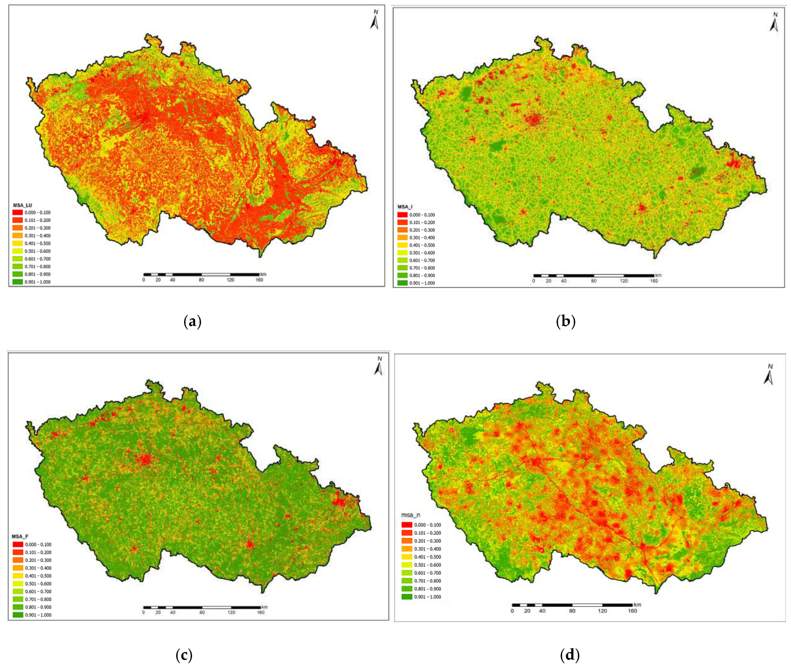
2.2.1. MSA of Land Use Change (MSA_LU)

Whereas in the original GLOBIO3 model, the main Global land cover classes are used to classify the MSA_LU from 0.05 (built-up area) to 1 (snow and ice, bare vegetation, forests) [11], we used the CL to calculate the MSA_LU for the territory of the CR. The quality of natural and near-natural habitats was valuated according to their representativeness and preservation following the Czech Habitat Assessment Methodology from 2000 to 2004 [49]. Representativeness expresses the extent to which the assessed habitat is identical to the description of the natural habitat type according to the Habitat catalogue of the Czech Republic [44]. Preservation assesses the state of the habitat from the perspective of nature conservation. In 2006, the Habitat mapping layer was updated with another methodology [50]. Two new evaluation characteristics were defined: representativeness and degree of degradation. The determination of representativeness differs from the old methodology by focusing on the phytocenological conformity of the evaluated stand with the habitat type. The degree of degradation expresses the intensity of the anthropogenic influence expressed by the presence of synanthropic species. The MSA_LU achieved the values 0.7 to 1 for natural habitats and 0.6 to 0.9 for near-natural habitats, according to both methodologies [49,50]. The range of values for degraded habitats was assigned according to Alkemade et al. [11]; the values of individual degraded habitats were estimated using the degree of naturalness and vulnerability of habitats [46] from 0.1 for anthropogenic habitats to 0.5 for distant natural habitats.

2.2.2. MSA of Infrastructure Development (MSA_I)

The value of MSA_I reached a lower value when infrastructure (mainly roads) was close to the assessed area, and therefore the impact of infrastructure on biodiversity was higher. Cities and agricultural land were not included in the original GLOBIO3 model [11]. However, in accordance with the aim of our study, we also calculated the infrastructure impact for urban and agricultural areas to evaluate the MSA_I for the whole CR. Infrastructure is defined as the road networks and built-up areas that form degraded habitats. We determined three parameters for each habitat to assess the load of its existing infrastructure. The first parameter was expressed as a direct impact of infrastructure and was defined as the distance from the infrastructure to the borders of the assessed area from 0 to 15 km, classified in several buffer zones. The second parameter expressed the sensitivity of the assessed area to the infrastructure on a scale from 1 as very sensitive, 2 as sensitive, and 3 as low-sensitive areas. The last parameter represented the population density, and it was expressed by the number of inhabitants per one square kilometer divided into three categories: 0–10, 10–50, and more than 50 inhabitants per square kilometer. All three parameters were calculated on a continuous scale according to Van Rooij [18] and appeared in GIS vector format. We performed spatial overlay operations between buffer zones, defining the specified distances of individual habitats from the infrastructure, classified by population density layer and habitat map with three levels of sensitivity. This was followed by attribute selection according to the combinations listed in

Table 2. The MSA_I values for individual combinations of sensitivity, buffer zone, and population density in the assessed area. This table was modified according to Van Rooij [18].

Very SensitiveAreas, Sensitivity Value = 1
Buffer zone (km)	0–0.5	0.5–1.0	1.0–1.5	1.5–3	3–4.5	4.5–5	5–10	10–15	>15
Density 0–10	0.5	0.75	0.75	0.9	0.9	0.9	1	1	1
Density 10–50	0.5	0.5	0.75	0.75	0.9	0.9	0.9	1	1
Density >50	0.5	0.5	0.5	0.75	0.75	0.9	0.9	0.9	1
SensitiveAreas, Sensitivity Value = 2
Buffer zone (km)	0–0.25	0.25–0.5	0.5–0.75	0.75–1.5	1.5–2.25	2.25–5	5–7.5		>7.5
Density 0–10	0.5	0.75	0.75	0.9	0.9	1	1		1
Density 10–50	0.5	0.5	0.75	0.75	0.9	0.9	1		1
Density >50	0.5	0.5	0.5	0.75	0.75	0.9	0.9		0.9
Low-Sensitive Areas,Sensitivity Value = 3
Buffer zone (km)	0–0.15	0.15–0.3	0.3–0.45	0.45–0.9	0.9–1.35	1.35–1.5	1.5–3	3–4.5	>4.5
Density 0–10	0.5	0.75	0.75	0.9	0.9	0.9	1	1	1
Density 10–50	0.5	0.5	0.75	0.75	0.9	0.9	0.9	1	1
Density >50	0.5	0.5	0.5	0.75	0.75	0.9	0.9	0.9	1

.

2.2.3. MSA of Fragmentation (MSA_F)

According to the original GLOBIO3 model, the most vulnerable areas of fragmentation are small areas of natural habitats that have the lowest MSA_F value. The least vulnerable areas are the large, protected areas and already degraded areas, such as arable land and cities that have the highest MSA_F value because they are not threatened by fragmentation [11]. In our CZ-GLOBIO modification, we kept the highest values of MSA_F for the large protected little fragmented areas and low values for highly fragmented natural and near-natural areas. However, unlike the original GLOBIO3, we also assigned low values to areas with low naturalness (for example, urban areas) because the current fragmentation impact cannot reduce their habitat naturalness further; these areas were almost fully fragmented during their transformation to anthropogenic habitats.

Fragmentation elements (roads, railways, buildings) were defined by Van Rooij [18], and individual types of habitats were merged according to the five types of habitat naturalness (natural, near-natural, distant natural, unnatural, and anthropogenic habitat groups). Subsequently, the merged habitats in the CL were divided into fragmentation elements, and the newly created areas of fragmented segments were calculated and divided by size into six categories (

Table 3. Value of the MSA_F for a detailed scale throughout the CR. The table was modified on the basis of Van Rooij [18] for the value of the MSA_F on a regional scale.

Area (km2)	MSAF
<0.5	0.3
1	0.6
2	0.7
4.5	0.9
10	0.95
>10	1

). This step created a layer with MSA_F values for the area of the whole CR. To express the MSA_F value of individual habitats, we cut this layer again according to the CL, and the average size of the fragmented segment of each habitat type was calculated.

2.2.4. MSA of Atmospheric Nitrogen Deposition (MSA_N)

The effect of nitrogen deposition was derived from critical load values for major ecosystems using a soil map and the sensitivity of ecosystems to nitrogen inputs. The nitrogen deposition driver was applied only to natural lands, not to croplands or urban areas [11]. We evaluated the nitrogen deposition from a nitrogen deposition map with 500 × 500 m pixels from 2007 for the whole territory of the CR (Zapletal, unpublished data). The empirical critical load value of nitrogen was calculated as the ratio between the number of ground vegetation species in N-treated habitat and species number in control habitats [36]. The critical load value was assessed for non-forest natural and near-natural habitats by Bobbink [36], Bobbink and Hettelingh [38], and Zapletal et al. [51]. For natural forest habitats, the critical load values calculated for long-term steady state conditions according to UBA [52] were assessed by Zapletal (unpublished data). The empirical critical load values for degraded habitats were derived from the percentage of remaining diagnostic species from the Habitat catalogue of the Czech Republic [44], corresponding to the nearest types of natural or near-natural habitats.

The value of nitrogen exceedance (NE) for each habitat was calculated as the difference between the atmospheric nitrogen deposition and the empirical critical load of nitrogen. Finally, we calculated the MSA_N value according to Equation (3) derived from Alkemade et al. [11] without coefficients for individual biomes if the value of NE was exceeded. An MSA_N with values less than 1 showed that the exceedance was higher than the buffering capacity of the ecosystem and its structure when diversity of plant species and ecosystem functioning were beginning to be disrupted or were already disrupted [36,51]. If the NE value was not exceeded, an MSA_N value close to 1 was assigned to the habitat.

MSA_N = 1 − ln (NE + 1)

(3)

3. Results

The outputs of the CZ-GLOBIO model are the MSA values of four main drivers, and they reflect the loss of naturalness and biodiversity vulnerability at the habitat level. The total MSA value (MSA_TOT2) was calculated as a space overlay of all layers of four MSA indicators for the whole CR (

Table 4. The mean values of MSA for all drivers and MSA_TOT2.

Values/MSA Indicators	MSALU	MSAI	MSAF	MSAN	MSATOT2
Weighted average of MSA	0.38	0.62	0.74	0.52	0.62
Number of habitat segments in the CR	2,051,876	8,781,992	580,983	6,329,639	33,133,951

For the abbreviations of the MSA indicators, see the legend below Table 1.

and

Table 5. The representation of each MSA indicator in the five intervals of the achieved MSA values (0–1).

Category	Interval of MSA Value (%)	MSALU %	MSAI %	MSAF %	MSAN %	MSATOT2 %
1	>0 and ≤0.2	41.8	8.2	6.8	12.17	6.12
2	>0.2 and ≤0.4	20	<1	14.9	20.13	10.01
3	>0.4 and ≤0.6	21	35.8	7	17.04	28.94
4	>0.6 and ≤0.8	7.8	38.5	9.3	15.62	47.28
5	>0.8 and ≤1	9.5	17.5	62	35.04	7.65

For the abbreviations of the MSA indicators, see the legend below Table 1.

; Figure 1 and Figure 2). The MSA values of all drivers and of MSA_TOT2 are presented in two ways. First, the average MSA value of each driver was calculated as a weighted average of the MSA values representing the areas of individual habitat types in the CR (Table 4). Second, we calculated the percentage of each MSA indicator represented in five intervals of MSA values from 0 to 1 (Table 5) to give a better overview of the pressure of each driver on the original biodiversity.

The average MSA_TOT2 value was 0.62. The MSA_LU indicator, characterizing the current naturalness of habitats, reached only the value 0.38 (a value of 1 represents the original state of habitat biodiversity). The remaining indicators of infrastructure development, fragmentation, and atmospheric nitrogen deposition reached higher MSA values (from 0.52 to 0.74) in the original habitat status. Concerning the representation of MSA indicators in five intervals of MSA values, the MSA_TOT2 value reached only 16% in the interval of MSA value from 0 to 0.4. The indicators MSA_LU and MSA_N reached a higher representation (62% and 32%) in the interval of MSA values from 0 to 0.4 compared to MSA_I (8%) and MSA_F (22%) (Table 5).

The highest values of all MSA indicators were found in the mountainous border zones and in the hilly parts in the military areas of the CR. These high values of MSA indicators mostly corresponded with the occurrence of large, protected areas. The lowest values of indicators were found in the vicinity of large cities and in arable land areas (Figure 1 and Figure 2).

We also assessed the MSA indicators of four selected drivers affecting the biodiversity for natural, near-natural, and degraded habitat types (distant natural, unnatural, and anthropogenic habitats) with the different degrees of naturalness established by Seják et al. [46]. The groups of natural and near-natural habitats reached the highest values of MSA_TOT2, ranging from 0.66 to 0.84. The MSA_LU values ranged from 0.72 to 0.98. The other three indicators (MSA_I, MSA_F, MSA_N) had a large range of MSA with values from 0.38 to 0.98 for groups of natural and near-natural habitats (

Table 6. The average values of MSA weighted by area for each group of natural and near-natural habitats. Habitat classification according to Chytrý et al. [44].

Category of Habitat Types	Groups of Natural, Near-Natural Habitats	MSALU	MSAI	MSAF	MSAN	MSATOT2
Grasslands	Alluvial meadows	0.72	0.67	0.48	1.00	0.76
	Dry meadows	0.75	0.67	0.52	0.99	0.77
	Mesic meadows	0.72	0.59	0.51	0.99	0.74
	Alpine grasslands	0.85	0.74	0.76	0.54	0.76
	Heaths	0.77	0.66	0.55	0.72	0.70
Forests	Alluvial forests	0.82	0.62	0.53	0.95	0.77
	Oak and oak–hornbeam forests	0.82	0.62	0.57	0.88	0.76
	Ravine forests	0.84	0.60	0.64	0.97	0.79
	Beech forests	0.84	0.66	0.64	0.87	0.78
	Dry pine forests	0.81	0.65	0.54	0.75	0.72
	Spruce forests	0.87	0.75	0.82	0.74	0.81
	Bog forests	0.85	0.69	0.75	0.66	0.76
	Native dwarf pine scrub	0.98	0.84	0.98	0.38	0.84
	Native shrub vegetation	0.73	0.59	0.46	0.78	0.68
Wetlands	Wetlands and littoral vegetation	0.73	0.63	0.46	0.73	0.68
	Peatbogs and springs	0.87	0.80	0.75	0.64	0.80
Rocks, rubble		0.83	0.60	0.64	0.40	0.66

For the abbreviations of the MSA indicators, see the legend below Table 1.

). The groups of distant natural habitats reached lower values of MSA_TOT2 ranging from 0.38 to 0.64, with MSA_LU values from 0.21 to 0.49. The groups of unnatural and anthropogenic habitats achieved the lowest values. The values for MSA_TOT2 ranged from 0.24 to 0.54, while MSA_LU values were from 0.10 to 0.28 (

Table 7. The average values of MSA weighted by area for each groups of degraded habitats (distant natural, unnatural, and anthropogenic habitat groups) classified according to Frélichová et al. [47].

Degree of Naturalness of Habitat	Category of Habitat Types	MSALU	MSAI	MSAF	MSAN	MSATOT2
Distant natural	Non-native dwarf pine	0.49	0.69	0.67	0.33	0.57
	Intensive mixed forests	0.46	0.59	0.60	0.63	0.63
	Intensive broad-leaved forests	0.43	0.49	0.65	0.48	0.54
	Anthropogenic swamps	0.42	0.62	0.71	0.38	0.58
	Intensive coniferous forests	0.42	0.66	0.55	0.53	0.63
	Introduced shrub vegetation	0.34	0.54	0.62	0.44	0.54
	Intensive grasslands	0.31	0.58	0.76	0.77	0.64
	Artificial rocks and quarries	0.21	0.36	0.65	0.25	0.38
Unnatural	Orchards and gardens	0.29	0.57	0.71	0.32	0.53
	Vineyard	0.28	0.51	0.44	0.27	0.45
	Hop fields	0.27	0.59	0.57	0.34	0.54
	Green urban areas (parks, gardens, cemeteries)	0.25	0.25	0.68	0.27	0.32
	Recreation sport areas	0.24	0.42	0.22	0.29	0.42
	Arable land	0.24	0.61	0.72	0.26	0.53
Anthropogenic	Discontinuous urban fabric	0.19	0.34	0.38	0.25	0.35
	Dumps and construction units	0.16	0.29	0.42	0.24	0.32
	Industrial and commercial units	0.12	0.22	0.26	0.22	0.27
	Transport network	0.12	0.40	0.49	0.24	0.37
	Continuous urban fabric	0.10	0.19	0.34	0.21	0.24

For the abbreviations of the MSA indicators, see the legend below Table 1.

).

Significant differences were also identified in the influence of the four drivers on the biodiversity of individual habitat groups according to the degree of their naturalness. The natural and near-natural habitat groups of mesic meadows and natural scrub vegetation were the most threatened by infrastructure development, whereas other habitat groups, such as native dwarf pine scrubs, spruce forests, peatbogs and springs, and alpine grasslands, were the least threatened by this driver. Non-forest habitat groups (alluvial, dry, mesic meadows and wetlands, and littoral vegetation) and forest habitat groups (alluvial forests, oak and oak–hornbeam forests, and natural shrub vegetation) were most threatened by fragmentation. Most habitats did not appear to be at risk of atmospheric nitrogen deposition, but the habitat groups that include rocks, rubble, native shrub vegetation, wetlands and littoral vegetation, and heaths were threatened by this driver (Table 6).

The distant natural habitat groups of artificial rocks and quarries, intensive grasslands, and introduced shrub vegetation were most threatened by land use change. On the other hand, habitat groups that include artificial rocks and quarries, anthropogenic swamps, and non-native dwarf pine were most affected by atmospheric nitrogen deposition. As we expected, unnatural and anthropogenic habitats had the lowest values of all MSA indicators (Table 7).

4. Discussion

The main aim of our study was to assess the loss of naturalness and the vulnerability of biodiversity at the habitat level on a detailed scale across the Czech Republic (CR) using the CZ-GLOBIO model derived from GLOBIO3. The MSA_TOT2 value was 0.62 but the mean values of individual MSA indicators ranged from 0.38 to 0.74 (Table 6 and Table 7). The values of MSA indicators provide information about the current transformation of natural and near-natural habitats into degraded habitats and their vulnerability to land use change, proximity to infrastructure, fragmentation, and atmospheric nitrogen deposition. The MSA indicators reached higher values of MSA_LU and MSA_N for groups of natural and near-natural habitats compared to distant natural habitat groups. This is caused by the degradation of naturalness of distant natural habitats, the reduction of their buffering capacity, and an increase in nitrogen deposition due to industry and automobile traffic [53]. On the other hand, MSA_F values were the same for natural and near-natural habitats and distant natural habitats while the MSA_I values for groups of distant natural habitats were higher than those for natural and near-natural habitats. Infrastructure development appears to have a greater effect on reducing biodiversity in natural and near-natural habitats [44] (Table 6). According to Stenhouse [54], these drivers can reduce the biodiversity of the last remnants of natural and near-natural habitats near large cities, even in nature reservations, through the fragmentation effect. It is possible to convert relatively easily distant natural habitats back to natural and near-natural habitats through revitalization processes [55]. However, inappropriate management or land use change can transform these habitats into unnatural or anthropogenic habitats according to by Ellenberg’s degradation series concept [56]. For this reason, it is necessary to monitor the entire spectrum of degradation and regradation series from natural and near-natural habitats to distant natural, unnatural, and anthropogenic habitats, as well as to maintain habitats with the highest degree of naturalness [57].

Only 16% of the MSA_TOT2 values were found in the interval from 0 to 0.4 for the whole CR. This occurred because the indicators MSA_I, MSA_F, and MSA_N ranged only from 8 to 32% in the MSA interval 0–0.4. This result was caused by the lower vulnerability of large-scale areas of distant natural and unnatural habitats to infrastructure development and fragmentation (Table 5 and Table 7).

We compared our results of the MSA values with other studies from the CR. Kaňková [27] calculated the MSA_TOT1 value from the same drivers without atmospheric nitrogen deposition but achieved only the value 0.2 for MSA_TOT1 in the CR compared with our MSA_TOT2 value of 0.62. This significant difference could be caused by two factors. First, Kaňková [27] used the original method on a global scale following Alkemade et al. [11], whereas we used the data on a detailed scale across the CR. Second, we used Equation (2) for calculating MSA_TOT2, whereas Kaňková [27] used Equation (1) according to Alkemade et al. [11]. This latter factor seems to be more influential. When we recalculated our MSA_TOT2 using Equation (1) for the same three MSA indicators as Kaňková [27], we achieved a similar MSA_TOT1 value of 0.17. When we recalculated the total MSA value from Kaňková’s [27] data using our Equation (2), the result of the MSA_TOT2 changed to 0.78.

We assume that it is more appropriate to use our modification of the MSA_TOT2 indicator through our Equation (2) when we have determined the MSA indicator on the basis of the naturalness of the habitats. Alkemade et al. [11] calculated the MSA indicator on the basis of the remaining species abundance compared to the abundance of original species in undisturbed ecosystems, and for this reason it was appropriate to use a version of Equation (1) that follows the central limit theorem in logarithmic space. If we apply Equation (1) of Alkemade et al. [11], the value of MSA_TOT1 reaches 0.1 of our four MSA indicators. However, it is possible to calculate the MSA_TOT value from the values of each MSA indicator to compare with any equation. Some studies only consider partial MSA indicators and drivers, or they did not count the MSA_TOT indicator. Trisurat [20] and Vačkář [25] evaluated only the land use change drivers. Meyer and McLean [21] assessed the effect of each of the five drivers on biodiversity separately and did not consider the MSA_TOT indicator.

Differences between our MSA_LU value (0.38), the result (0.26) from Kaňková [27], and the result (0.31) from Vačkář et al. [25] based on data of a similar scale were smaller. Recently, Vačkářů and Grammatikopoulou [26] compared the calculation of MSA_LU from regional-scale data (CORINE LC) and on a detailed scale across the CR (Consolidated Layer of Ecosystems) without finding significant differences. Compared to our results, Kaňková’s results [27] for the two remaining MSA indicators (MSA_I, MSA_F) reached the higher values of 0.95 and 0.93, respectively. This was due to the fact that the fragmentation and infrastructure development drivers were counted only in areas where the MSA_LU values were higher than 0.5. The main reason was the assumption that these two drivers significantly impact natural and near-natural areas [27].

The MSA_TOT1 calculated in other studies using Equation (1) according to Alkemade et al. [11] reached the values of 0.26 in Vietnam [22], 0.52 in Thailand [20], and 0.55 in Zambia [18]. Land use change, infrastructure development, and fragmentation could reduce the MSA_TOT1 value in the future on the basis of the model prediction calculated by Trisurat et al. [20] since deforestation in particular can also affect protected areas. In our study, we found the lowest values for land use change produced the lowest values. The values then increased with atmospheric nitrogen deposition, infrastructure development, and finally fragmentation. The main reason for the higher impact of atmospheric nitrogen deposition could be the growth of urban areas associated with infrastructure development [58,59] and the distant transport of pollution to higher altitudes [60]. According to Trisurat et al. [20], the highest MSA_TOT1 value is associated with high altitude and inaccessible areas. In line with this finding, we observed the highest MSA_TOT2 value in the mountains with high altitudes along the CR state border (Figure 1 and Figure 2), especially in large protected areas such as national parks, landscape protected areas, and military areas with limited settlements [61]. Similarly, Vačkář et al. [25] revealed higher MSA_LU values in large-scale protected areas with a higher proportion of natural habitats (0.48) than in non-protected cultural forest–agriculture landscapes (0.28).

The additional aim of our study was to determine the vulnerability of habitat types according to the individual drivers. Threats differed for each driver and naturalness type of natural, near-natural, and degraded habitats. According to our results, the mean values of MSA_LU for the whole CR reached only 0.38. This corresponds to historical land use changes. After 1950, due to the communist regime, these changes mainly involved the collectivization of agricultural land and the centralization of its management, resulting in large blocks of arable land and the elimination of grassland boundaries and hedgerows. In many areas, nearly 800,000 ha of agricultural land was converted from grassland to arable land and/or drainage [62]. Later, since the regime change in 1989, progressive urbanization and construction of commercial centers took place [53,63,64], resulting in permanent loss of high quality arable land. Among the most significant changes since 1989 has been the conversion of low-quality arable land to grassland, which was encouraged by subsidies after 2000. Almost 50% of grassland in 2010 was in the less -favored areas with higher elevations and steeper slopes [65]. However, habitat quality was also declining in grasslands. Floodplain meadows were either converted into managed meadows, pastures, and arable land, or they were used for construction. A similar situation exists today in Slovakia [66] and in northern Germany [67].

Infrastructure development connected with fragmentation have reduced the biodiversity of many natural, near-natural, and distant natural habitats, especially native and introduced shrub vegetation habitats along roads, which are affected by regular cutting and new communication lines. The road network also reduces the quality of natural habitats with the spreading of weeds and invasive plants [68]. Highway construction has led to the additional occupation of adjacent habitats 75 m from the edge of the highways themselves caused by changes in the heat balance [69], and 200 m from the edge as a result of the secondary development of commercial and residential areas [59]. The share of unfragmented areas decreased from 81% in 1980 to 64% in 2005 due to road transport across the CR, and the average size of individual unfragmented areas also decreased from 307 km² in 1980 to 218 km² in 2005 [70]. These figures show that infrastructure with accompanying fragmentation has a strong impact on reducing the naturalness of habitats. However, in our study, infrastructure accompanied with fragmentation had the strongest influence on the anthropogenic habitat groups and also on the unnatural habitat group such as urban green spaces and recreational sports areas. These results are related to the establishment of infrastructure and fragmentation drivers. The driver infrastructure was expressed by the direct influence of infrastructure (roads, railways), the sensitivity of the assessed area to infrastructure, and the population density expressed by the number of inhabitants per one square kilometer. A fragmentation driver is associated with the infrastructure driver. This driver was expressed by the size of habitats and their degree of naturalness. The highest values of MSA_F had large protected and low fragmented areas, while low values had highly fragmented natural and semi-natural areas and areas with low naturalness (e.g., urban areas). This phenomenon could be due to the connection of habitat blocks with the same degree of naturalness, which then form larger complexes (Table 4).

Infrastructure development and fragmentation have affected grassland habitats (especially meadows of all types) more than forest habitats in Central Europe due to long-term human management [71]. The least affected natural forest habitats are native dwarf pine scrubs and spruce forests due to their occurrence in inaccessible locations such as large, protected areas (Table 6). However, fragmentation of the forest landscape caused by the development of the road network between 1960 and 2016 significantly reduced the compact forest habitats in large, protected areas such as the Šumava NP and the Krkonoše Mountains NP [64]. Further, the habitats of alluvial forests and oak and oak–hornbeam forests are most likely to be threatened by fragmentation and infrastructure, probably due to their occurrence in cultural forest–agriculture landscape near settlements and infrastructure development.

Atmospheric nitrogen deposition had the highest impact on habitats of native dwarf pine scrub, rocks, screes, and alpine grasslands occurring in high mountains with an elevated atmospheric nitrogen deposition due to distant transport. This process started 40 years ago in the Krkonoše Mts. [72] and Jeseníky Mts. [60]. In the Krkonoše Mts., the deposition of SO₂ rapidly decreased after the desulphurization of coal power stations during the years 1990–2000 [73], whereas nitrogen deposition still significantly exceeded the critical load for nutrient nitrogen in 2005 [74]. Nevertheless, spruce forest habitats have slowly started to regenerate in the Krkonoše Mts. The authors of [38] found that there was a lower empirical critical load value of nitrogen (5–15 kg N ha⁻¹ year⁻¹) for native dwarf pine scrubs and alpine grasslands than for spruce forest habitats (10–15 kg N ha⁻¹ year⁻¹). This wide range of values was determined by analyzing either changes and decline in plant species composition or the decreased biomass of fine roots and soil fauna. Using long-term steady-state conditions (Zapletal, unpublished data), we found that the critical load value for the natural habitats of spruce forests was 11–12 kg N ha⁻¹ year⁻¹.

Atmospheric nitrogen deposition has also had a significant influence on unnatural habitats such as arable land, vineyards, recreation sport areas, and green urban areas, as well as on anthropogenic habitats such as discontinuous urban fabric, continuous and discontinuous urban fabric, industrial and commercial units, transport networks, and dumps and construction units. The MSA_N values ranged only from 0.21 to 0.29 due to the high amount of atmospheric deposition, while the empirical critical load value of nitrogen ranged from 1 to 3 kg N ha⁻¹ year⁻¹. These values concur with the current finding that the largest sources of nitrogen are automobile traffic [75] and big cities [76]. However, the most natural, near-natural, and distant natural habitats were less affected by the nitrogen driver and reached an MSA_N value in the range from 0.44 to often more than 0.6. The MSA_N indicator reached the values 0.25–0.40 only a few times for habitats of rocks, rubble, anthropogenic swamps, artificial rocks, and quarries. According to Chytrý et al. [44], the habitats of tall grasslands on rock ledges and habitat tall-sedge beds are threatened by eutrophication, which is currently caused by the atmospheric nitrogen deposition. These findings concur with the results of Kolář et al. [77], who evidenced a reduction of nitrogen oxide emissions across the Czech Republic after 1990, together with a decreased in the fertilization rate of farmland, particularly fields [78]. However, atmospheric nitrogen deposition has remained at a significantly high level, mainly in the forests [79].

According to our results, the total value of the MSA_TOT2 indicator for CR is still high (0.62). However, the low values of MSA_LU show a distinct decrease in biodiversity compared to the original natural habitats as confirmed by Sklenicka [58], Kaňková [24], and Vačkář et al. [25]. Land transformation for intensive agriculture, forestry plantations, and urbanization both in the CR and worldwide has been the most significant reason for biodiversity loss. For biodiversity loss to be reduced at the habitat level, it is necessary to effectively protect natural and near-natural habitats, consider the sustainable use of arable land, and establish plantation forestry on degraded land [11].

The main limitation of our investigation concerns the interpretation of the CZ-GLOBIO results due to inaccurate input data. Although we tried to work with the most recent data available, most of the data used were not older than 10 years. Therefore, we assume that with more recent data, the values of some drivers would probably be different, especially for the land use change driver. Similarly, we tried to use the most detailed classification of land use available in the Czech Republic regarding the variability of environmental conditions of Central Europe and their frequent changes under the influence of natural and socio-economic drivers [53,65]. Because it was problematic to obtain data on the loss of biodiversity in comparison with natural communities, we assessed habitat naturalness using the expert method of “Biotope Valuation Method” [46]. We consider not using the available plant database data for the CR because these data have a variable distribution in space and highly variable time records. Therefore, it is not possible to use these species data to describe the condition of habitats in a defined time period for which we are assessing the condition of threats to landscape biodiversity in the CR. For this reason, we used habitat type assessment data from habitat mapping in the CR. The methodology of habitat mapping in the Natura2000 system at the Czech Republic is largely compatible with Europe-wide mapping [49,50]. Automation of processing of heterogeneous input data and processing of a large number of spatial combinations (segments of individual drivers have a size of units up to tens of millions) are solvable only with the use of spatially oriented software tools. For our CZ-GLOBIO model, we used the ArcGIS Pro software. With this software, it is possible to process data at a detailed scale for the entire Czech Republic in a relatively short time (on the order of 10 h).

We are working on the creation of a climate change driver for the CZ-GLOBIO model using EUROMOVE module. The impacts of climate change are more likely to affect habitats that are in extreme conditions, such as alpine mountain grasslands, dry grasslands, and peat bogs. An increase in temperature with the same amount of precipitation will also have a negative impact on habitats that already occur in dry areas, e.g., South Moravia. At the same time, a change in climatic conditions may lead to a more intensive spread of alien and invasive species downstream of transport routes and watercourses. A more accurate prediction of the response of individual habitats to changes in climatic conditions needs to be made only after the driver of climate change has been incorporated into the CZ-GLOBIO model.

On the basis of our investigation, we propose the adaptation of the assessment of the MSA indicators to habitat naturalness and using the CZ-GLOBIO model for political decision-making on biodiversity protection at the national level. The habitat quality is a good proxy for biodiversity status, and land use data about habitat occurrences are easily available to the government [80]. In the CR context, in order to include the CZ-GLOBIO model in the decision-making processes of the state administration, we recommend applying the most up-to-date data on driver impacts, on the state of land use, and on natural habitat occurrences. Habitat mapping is regularly updated via surveillance following the Habitat Directive obligations by the Nature Conservation Agency of the Czech Republic [81].

5. Conclusions

The GLOBIO3 model has been modified to CZ-GLOBIO to assess the loss of naturalness and current vulnerability of biodiversity at the habitat level in the Czech Republic at the scale 1:10,000. The main reason was the need for more detailed data to determine the loss of biodiversity in time and space for all habitats in the Czech Republic. Therefore, we also changed the original Equation (1) used to calculate the MSA_TOT1 of Alkemade et al. [11] to Equation (2). We applied the four drivers of land use change, infrastructure development, fragmentation, and atmospheric nitrogen deposition. The MSA_TOT2 calculated from the spatial overlay of the four MSA indicators reached 0.62 according to our version of Equation (2), and according to Equation (1), the MSA_TOT1 reached the value 0.1 for the whole Czech Republic. On the basis of a comparison of MSA_TOT values from two different equations, we recommend using MSA_TOT to compare landscape segment values within a one study and using individual MSA indicators to compare biodiversity loss between studies.

The highest values of all MSA indicators were found in the naturally protected mountains with high slopes in the border zone and in the hilly parts in the military areas of the CR. In these areas, the negative impact of humans on habitats was lower in the past due to the more difficult accessibility of these areas. Moreover, a large part of these areas is currently designated as protected areas [25].

Natural and near-natural habitats are threatened by infrastructure development and fragmentation. These drivers can reduce the biodiversity of the last remnants of natural and near-natural habitats near large cities, even in nature reserves. Distant natural habitats are threatened by land use change and atmospheric nitrogen deposition. These habitats can relatively easily be converted to natural and near-natural habitats through revitalization measures, but they are at risk of becoming unnatural or anthropogenic habitats through inappropriate management or land use change. Nevertheless, the MSA_TOT2 value for distant natural habitats has decreased by 25% compared to the MSA_TOT2 for natural and near-natural habitats. The important land use change driver reached only the value 0.38 for the CR, but this finding is in accordance with the results of other local studies.

For the loss of biodiversity to be reduced at the habitat level, it is necessary to better control urban development and to protect more intensively the residues of natural and near-natural habitats. The modified CZ-GLOBIO model based on the quality of habitats seems to be a suitable tool for political decision making on biodiversity protection at the national level. For the GLOBIO model to be successfully applied, however, it is necessary to use up-to-date detailed data of the state of biodiversity and individual drivers of biodiversity loss in the areas of interest. Using the CZ-GLOBIO model in ArcGIS software, we are able to process input data at a detailed scale for the entire Czech Republic in a relatively short time.

References

1. Salafsky, N.; Salzer, D.; Stattersfield, A.J.; Hilton-Taylor, C.; Neugarten, R.; Butchart, S.H.M.; Collen, B.; Cox, N.; Master, L.L.; O’Connor, S.; et al. A standard lexicon for biodiversity conservation: Unified classifications of threats and actions. Conserv. Biol. 2008, 22, 897–911. [Google Scholar] [CrossRef] [PubMed]
2. Pereira, H.M.; Leadley, P.W.; Proenca, V. Scenarios for Global Biodiversity in the 21st Century. Science 2010, 330, 1496–1501. [Google Scholar] [CrossRef] [PubMed] [Green Version]
3. Kok, M.; Alkemade, R. How Sectors Can Contribute to Sustainable Use and Conservation of Biodiversity. Secretariat of the Convention on Biological Diversity; Technical Series 79; PBL Netherlands Environmental Assessment Agency: Hague, The Netherlands, 2014; 230p.
4. Fischer, M.; Rounsevell, M.; Torre-Marin Rando, A.; Mader, A.D.; Church, A.; Elbakidze, M.; Elias, V.; Hahn, T.; Harrison, P.A.; Hauck, J.; et al. Summary for Policymakers of the Regional Assessment Report on Biodiversity and Ecosystem Services for Europe and Central Asia of the Intergovernmental Science-Policy Platform on Biodiversity and Ecosystem Services; IPBES Secretariat: Bonn, Germany, 2018; 48p. [Google Scholar]
5. Scholes, R.J.; Biggs, R. A biodiversity intactness index. Nature 2005, 434, 45–49. [Google Scholar] [CrossRef] [PubMed]
6. MEA. Millennium Ecosystem Assessment. Ecosystems and Human Well-Being. Synthesis; Island Press: Washington, DC, USA, 2005; 155p.
7. CICES. Available online: https://cices.eu/cices-structure/ (accessed on 16 March 2020).
8. TEEB. Available online: http://www.teebweb.org/resources/ecosystem-services/ (accessed on 16 March 2020).
9. Scholes, R.; Montanarella, L.; Brainich, A.; Barger, N.; ten Brink, B.; Cantele, M.; Erasmus, B.; Fisher, J.; Gardner, T.; Holland, T.G.; et al. Summary for Policymakers of the Assessment Report on Land Degradation and Restoration of the Intergovernmental Science-Policy Platform on Biodiversity and Ecosystem Services; IPBES Secretariat: Bonn, Germany, 2018; 44p. [Google Scholar]
10. Leadley, P.W.; Krug, C.B.; Alkemade, R.; Pereira, H.M.; Sumaila, U.R.; Walpole, M.; Marques, A.; Newbold, T.; Teh, L.S.L.; van Kolck, J.; et al. Progress towards the Aichi Biodiversity Targets: An Assessment of Biodiversity Trends, Policy Scenarios and Key Actions; Technical Series 78; Secretariat of the Convention on Biological Diversity: Montreal, QC, Canada, 2014; 502p.
11. Alkemade, R.; van Oorschot, M.; Miles, L.; Nellemann, C.; Bakkenes, M.; ten Brink, B. GLOBIO3: A Framework to Investigate Options for Reducing Global Terrestrial Biodiversity Loss. Ecosystems 2009, 12, 374–390. [Google Scholar] [CrossRef] [Green Version]
12. Brink, B. Biodiversity Indicators for the OECD Environmental Outlook and Strategy: A feasibility Study; RIVN Report; National Institute of Public Health and the Environment: Bilthoven, The Netherlands, 2000; 52p. [Google Scholar]
13. Majer, J.D.; Beeston, G. The biodiversity Integrity Index: An illustration usingants in Western Australia. Conserv. Biol. 1996, 10, 65–73. [Google Scholar] [CrossRef] [Green Version]
14. Andreasen, J.K.; O’Neill, R.V.; Noss, R.; Slosser, N.C. Considerations for the development of a terrestrial index of ecological integrity. Ecol. Indic. 2001, 1, 21–35. [Google Scholar] [CrossRef]
15. Loh, J.; Green, R.E.; Ricketts, T.; Lamoreux, J.; Jenkins, M.; Kapos, V.; Randers, J. The living planet index: Using species population time series to track trends in biodiversity. Philosophical Transactions of the Royal Society of London B. Biol. Sci. 2005, 360, 289–295. [Google Scholar] [CrossRef] [PubMed] [Green Version]
16. Schipper, A.; Bakkenes, M.; Meijer, J.; Alkemade, R.; Huijbregts, M. The GLOBIO Model. A Technical Description of Version 3.5; PBL Netherlands Environmental Assessment Agency: Hague, The Netherlands, 2016; 36p.
17. Schipper, A.; Hilbers, J.P.; Meijer, J.; Antao, L.H.; Benítez-López, A.; de Jonge, M.M.J.; Leemans, L.H.; Scheper, E.; Alkemade, R.; Doelman, J.C.; et al. Projecting terrestrial biodiversity intactness with GLOBIO4. Glob. Chang. Biol. 2020, 26, 760–771. [Google Scholar] [CrossRef] [PubMed] [Green Version]
18. Van Rooij, W. Manual for Biodiversity Modelling on a National Scale. Using GLOBIO3 and CLUE Methodology to Calculate Current and Future Status of Biodiversity; Case study area: Zambia; PBL Netherlands Environmental Assessment Agency: Bilthoven, The Netherlands, 2008; 25p.
19. Glomsrød, S.; Duhaime, G.; Aslaksen, I. The Economy of the North 2015; Statistics Norway: Oslo–Kongsvinger, Norway, 2017; 172p.
20. Trisurat, Y.; Alkemade, R.; Verburg, P.H. Projecting Land-Use Change and Its Consequences for Biodiversity in Northern Thailand. Environ. Manag. 2010, 45, 626–639. [Google Scholar] [CrossRef] [PubMed] [Green Version]
21. Meyer, S.T.; McLean, D. Current and Future Status of Biodiversity in Central America. Technical Report, Strategic Biodiversity Monitoring and Evaluation Program (PROMEBIO); Central America Commission for Environment and Development: Mexico City, Mexican, 2011; 208p. [Google Scholar]
22. Son, V.T. Biodiversity assessment and modeling: Review and potential application in Vietnam. In Proceedings of the GeoInformatics for Spatial-Infrastructure Development in Earth and Allied Sciences (GIS-IDEAS), Hanoi, Vietnam, 4–6 December 2008. [Google Scholar]
23. Mücher, C.A.; van der Meer, P.J. Widening the Analytical Scope of GLOBIO3—Modeling Global Biodiversity; Project Biodiversity International of the Netherlands Environmental Assessment Agency (MNP); PBL Netherlands Environmental Assessment Agency: Hague, The Netherlands, 2006.
24. Kaňková, H. Assessment of human pressure on forest ecosystems in the Czech Republic. In Proceedings of the Bionature 2015, The Sixth International Conference on Bioenvironment, Biodiversity and Renewable Energie, IARA, Rome, Italy, 24–29 May 2015; pp. 34–35. [Google Scholar]
25. Vačkář, D.; Hamáčková, V.Z.; Kaňková, H.; Stupková, K. Human transformation of ecosystems: Comparing protected and unprotected areas with natural baselines. Ecol. Indic. 2016, 66, 321–328. [Google Scholar] [CrossRef]
26. Vačkářů, D.; Grammatikopoulou, I. Toward development of ecosystem asset accounts at the national level. Ecosyst. Health Sustain. 2019, 5, 1–11. [Google Scholar] [CrossRef]
27. Kaňková, H. Assesment of Land Use Influence on Landscape Naturalness. Master’s Thesis, Charles University, Prague, Czech Republic, 2013. [Google Scholar]
28. Stržínek, F. Multiscale Application of the Model GLOBIO. Master’s Thesis, Palacky University in Olomouc, Olomouc, Czech Republic, 2018. [Google Scholar]
29. Trisurat, Y.; Shrestha, R.P.; Alkemade, R. Land Use, Climate Change and Biodiversity Modeling: Perspectives and Applications, 1st ed.; IGI Global: Hershey, PA, USA, 2011; 512p. [Google Scholar]
30. UNEP. GLOBIO. Global Methodology for Mapping Human Impacts on the Biosphere; Report UNEP/DEWA/TR 25; United Nations Environment Programme: Nairobi, Kenya, 2001; 48p. [Google Scholar]
31. Verboom, J.; Snep, R.P.H.; Stouten, J.; Pouwels, R.; Pe’er, G.; Goedhart, P.W.; van Adrichem, M.H.C.; Alkemade, J.R.M.; Jones-Walters, L.M. Using Minimum Area Requirements (MAR) for Assemblages of Mammal and Bird Species in Global Biodiversity Assessments; Research Reports; Alterra: Wageningen, The Netherlands, 2014; 22p. [Google Scholar]
32. Woodroffe, R.; Ginsberg, J.R. Edge effects and the extinction of populations inside protected areas. Science 1998, 280, 2126–2128. [Google Scholar] [CrossRef] [PubMed] [Green Version]
33. Allen, C.R.; Pearlstine, L.G.; Kitchens, W.M. Modeling viable mammal populations in gap analyses. Biol. Conserv. 2001, 99, 135–144. [Google Scholar] [CrossRef] [Green Version]
34. Bouwman, A.F.; Van Vuuren, D.P.; Derwent, R.G.; Posch, M. A global analysis of acidification and eutrophication of terrestrial ecosystems. Water Air Soil Pollut. 2002, 141, 349–382. [Google Scholar] [CrossRef]
35. Verboom, J.; Alkemade, R.; Klijn, J.; Metzger, M.J.; Reijnen, R. Combining biodiversity modeling with political and economic development scenarios for 25 EU countries. Ecol. Econ. 2007, 22, 267–276. [Google Scholar] [CrossRef]
36. Bobbink, R. Plant Species Richness and the Exceedance of Empirical Nitrogen Critical Loads: An Inventory; Manuskript; Utrecht University: Utrecht, The Netherlands, 2004; 20p. [Google Scholar]
37. Bobbink, R.; Hicks, K.; Galloway, J.; Spranger, T.; Alkemade, R.; Ashmore, M.; de Vries, W. Global assessment of nitrogen deposition effects on terrestrial plant diversity: A synthesis. Ecol. Appl. 2010, 20, 30–59. [Google Scholar] [CrossRef] [PubMed] [Green Version]
38. Bobbink, R.; Hettelingh, J.P. Review and revision of empirical critical loads and dose-response relationships. In Proceedings of the an Expert Workshop (EUNIS), Noordwijkerhout, The Netherlands, 23–25 June 2010; B-WARE Research Centre: Noordwijkerhout, The Netherlands, 2011. [Google Scholar]
39. Midolo, G.; Alkemade, R.; Schipper, A.M.; Benítez-López, A.; Perring, M.P.; De Vries, W. Impacts of nitrogen addition on plant species richness and abundance: A global meta-analysis. Glob. Ecol. Biogeogr. 2018, 28, 398–413. [Google Scholar] [CrossRef] [Green Version]
40. Bakkenes, M.; Alkemade, J.R.M.; Ihle, F.; Leemans, R.; Latour, J.B. Assessing effects of forecasted climate change on the diversity and distribution of European higher plants for 2050. Glob. Chang. Biol. 2002, 8, 390–407. [Google Scholar] [CrossRef]
41. Bakkenes, M.; Eickhout, B.; Alkemade, R. Impacts of different climate stabilisation scenarios on plant species in Europe. Glob. Environ. Chang. 2006, 16, 19–28. [Google Scholar] [CrossRef]
42. Leemans, R.; Eickhout, B. Another reason for concern: Regional and global impacts on ecosystems for different levels of climate change. Glob. Environ. Chang. Hum. Policy Dimens. 2004, 14, 219–228. [Google Scholar] [CrossRef]
43. Cudlín, P.; Pechanec, V.; Štěrbová, L.; Cudlín, O.; Purkyt, J. Integrated approach to the mitigation of biodiversity lost in Central Europe. In Ecological Integrity and Land Use: Sovereignty, Governance, Displacements and Land Grabs; Westra, L., Bosselmann, K., Zabrano, V., Eds.; Nova Science Publishers: New York, NY, USA, 2019; pp. 75–86. [Google Scholar]
44. Chytrý, M.; Kučera, T.; Kočí, M.; Grulich, V.; Lustyk, P. Catalog of Habitats of the Czech Republic, 2nd ed.; Nature Conservation Agency of the Czech Republic: Prague, Czech Republic, 2010; p. 447. [Google Scholar]
45. The Occurrence of Natural Habitat in the Czech Republic. NCA CR, Habitat Mapping Layer (Electronic Database), Version 2014; Nature Conservation Agency of the Czech Republic: Prague, Czech Rapublic, 2014. [Google Scholar]
46. Seják, J.; Dejmal, I.; Petříček, V.; Cudlín, P.; Míchal, I.; Černý, K.; Kučera, T.; Vyskot, I.; Strejček, J.; Cudlínová, E. Assessment and Valuation of Habitats Czech Republic, 1st ed.; Czech Environmental Institute, Ministry of the Environment: Prague, Czech Republic, 2003; 422p. [Google Scholar]
47. Frélichová, J.; Vačkář, D.; Pártl, A.; Loučková, B.; Harmáčková, Z.; Lorencová, E. Integrated assessment of ecosystem services in the Czech Republic. Ecosyst. Serv. 2014, 8, 110–117. [Google Scholar] [CrossRef]
48. Pechanec, V.; Machar, I.; Štěrbová, L.; Prokopová, M.; Kilianová, H.; Chobot, K.; Cudlín, P. Monetary Valuation of Natural Forest Habitats in Protected Areas. Forests 2017, 8, 427. [Google Scholar] [CrossRef] [Green Version]
49. Guth, J. Natura 2000 and Emerald Habitat Mapping Methodologies (Detailed and Contextual Mapping Methodologies), 3rd ed.; Nature Conservation Agency of the Czech Republic: Prague, Czech Republic, 2002; p. 22. [Google Scholar]
50. Lustyk, P.; Guth, J. Methodology for Updating the Habitat Mapping Layer; Manuscript; Nature Conservation Agency of the Czech Republic: Praha, Czech, 2009; p. 31. [Google Scholar]
51. Zapletal, M.; Skořepová, I.; Buriánek, V. The Condition of Forest Soils as A Determining Factor in The Development of Health Status, Biodiversity and the Fulfillment of Production and Non-Production Functions of Forests; Report on the Progress of the Project NAZV QI112A168; Forestry and Game Management Research Institute: Prague, Czech Republic, 2014. [Google Scholar]
52. UBA. Manual on Methodologies and Criteria for Modelling and Mapping Critical Loads and Levels and Air Pollutions Effects, Risks and Trends; Federal Environmental Agency (Umweltbundesamt): Berlin, Germany, 2004; Texte 52/04. [Google Scholar]
53. Skokanová, H.; Falťan, V.; Havlíček, M. Driving forces of main landscape change processes from past 200 years in Central Europe—Differences between old democratic and post-socialist countries. Ekológia (Bratisl.) 2016, 35, 50–65. [Google Scholar] [CrossRef] [Green Version]
54. Stenhouse, R.N. Fragmentation and internal disturbance of native vegetation reserves in the Perth metropolitan area, Western Australia. Landsc. Urban Plan. 2004, 68, 389–401. [Google Scholar] [CrossRef]
55. Clewell, F.; Aronson, J. Ecological Restoration, Second Edition. Principles, Values, and Structure of an Emerging Profession, 2nd ed.; Island Press: Washington, DC, USA, 2013; 336p. [Google Scholar]
56. Ellenberg, H. Vegetation Mitteleuropas Mit den Alpen, in Kausaler, Dynamischer Und Historischer Sicht, 1st ed.; Eugen Ulmer: Stuttgart, Germany, 1963; 981p. [Google Scholar]
57. Seják, J.; Cudlín, P. On measuring the natural and environmental resource value and damages. Studia Ecol. 2010, 4, 53–68. [Google Scholar]
58. Sklenicka, P.; Molnarova, K.; Pixova, K.C.; Salek, M.E. Factors affecting farmland prices in the Czech Republic. Land Use Policy 2013, 30, 130–136. [Google Scholar] [CrossRef]
59. Keken, Z.; Sebkova, M.; Skaloš, J. Analyzing land cover change—The impact of the motorway construction and their operation on landscape structure. J. Geogr. Inf. Syst. 2014, 6, 559–571. [Google Scholar] [CrossRef] [Green Version]
60. Zapletal, M.; Chroust, P.; Kunak, D. The relationship between defoliation of Norway spruce and atmospheric deposition of sulphur and nitrogen compounds in Hruby Jesenik Mountains (the Czech Republic). Ecology 2003, 22, 337–347. [Google Scholar]
61. Cudlín, O.; Pechanec, V.; Purkyt, J.; Chobot, K.; Salvati, L.; Cudlín, P. Are valuable and representative natural habitats sufficiently protected? Application of Marxan model in the Czech Republic. Sustainability 2020, 12, 402. [Google Scholar] [CrossRef] [Green Version]
62. Vopravil, J.; Khel, T.; Vrabcová, T. Soil and Its Evaluation in the Czech Republic, Part I; Research Institute of Land Reclamation and Soil Protection: Prague, Czech Republic, 2009; 148p. [Google Scholar]
63. Smolová, I.; Szczyrba, Z. Large commercial centers in the Czech Republic–landscape and regionally aspects of development (contribution to the study of the problematic). Acta Univ. Palacki. Olomuc. Geogr. 2000, 36, 81–87. [Google Scholar]
64. Kupková, L.; Bičík, I. Landscape transition after the collapse of communism in Czechia. J. Maps 2016, 12, 526–531. [Google Scholar] [CrossRef]
65. Stych, P.; Kabrda, J.; Bicik, I.; Lastovicka, J. Regional Differentiation of Long-Term Land Use Changes: A Case Study of Czechia. Land 2019, 8, 165. [Google Scholar] [CrossRef] [Green Version]
66. Halada, L.; Ružičková, H.; David, S.; Halabuk, A. Semi-natural grasslands under impact of changing land use during last 30 years: Trollio-Cirsietum community in the Liptov region (N Slovakia). Community Ekol. 2008, 9, 115. [Google Scholar]
67. Krause, B.; Culmsee, H.; Wesche, K.; Bergmeier, E.; Leuschner, C. Habitat loss of floodplain meadows in north Germany since the 1950s. Biodivers. Conserv. 2011, 20, 2347–2364. [Google Scholar] [CrossRef] [Green Version]
68. Šerá, B. Road vegetation in Central Europe—An example from the Czech Republic. Biologia 2008, 63, 1085–1088. [Google Scholar] [CrossRef]
69. Nedbal, V.; Brom, J. Impact of highway construction on land surface energy balance and local climate derived from LANDSAT satellite data. Sci. Total Environ. 2018, 633, 658–667. [Google Scholar] [CrossRef] [PubMed]
70. Anděl, P.; Andreas, M.; Gorčicová, I.; Hlaváč, V.; Mináriková, T.; Romportl, D.; Strnad, M.; Zieglerová, A. The Concept of Protection of Migration Corridors of Large Mammals and the Territorial System of Ecological Stability; Proceedings of ÚSES-Green Backbone of the Landscape; The Silva Tarouca Research Institute for Landscape and Ornamental Gardening: Kostelec nad Černými lesy, Czech Republic, 2009; pp. 1–8. [Google Scholar]
71. Hejcman, M.; Hejcmanová, P.; Pavlů, V.; Beneš, J. Origin and history of grasslands in Central Europe—A review. Grass Forage Sci. 2013, 68, 345–363. [Google Scholar] [CrossRef]
72. Romportl, D. (Ed.) Final Report for 2018 on the Contract on the Implementation and Provision of Activities and Services in the Public Contract “Biological Research and Monitoring at the Landscape Level of the Czech Republic—Providing Professional Support for the Activities of the Ministry of the Environment. Part D: Changes in the Landscape and Trends in Landscape Development; The Silva Tarouca Research Institute for Landscape and Ornamental Gardening: Prague, Czech Republic, 2018. [Google Scholar]
73. Vacek, S.; Bílek, L.; Schwarz, O.; Hejcmanová, P.; Mikeska, P. Effect of air pollution on the health status of spruce stands. A case study in the Krkonoše Mountains, Czech Republic. Mt. Res. Dev. 2013, 33, 40–50. [Google Scholar] [CrossRef]
74. Hošek, J.; Schwarz, O.; Svoboda, T. Results of a ten-year measurement of atmospheric deposition in the Krkonoše Mountains. In Geoecological Problems of the Krkonoše Mountains, 1st ed.; Štursa, J., Knapik, R., Eds.; Sborník Mez. Věd. Konf.: Svoboda nad Úpou, Czech Republic, 2006; pp. 179–191. [Google Scholar]
75. Jandová, V.; Dostál, I.; Pelikán, L.; Špička, L.; Ličbinský, R. Study on Transport Trends from Environmental Viewpoints in the Czech Republic 2017; Transport Research Centre: Brno, Czech Republic, 2018; 191p. [Google Scholar]
76. Sejak, J.; Cudlin, P.; Pokorny, J.; Zapletal, M.; Petricek, V.; Guth, J.; Chuman, T.; Romportl, D.; Skorepova, I.; Vacek, V.; et al. Assessment of Ecosystem Functions and Services in the Czech Republic, 1st ed.; University, J.E., Ed.; Purkyne: Usti nad Labem, Czech Republic, 2010; 197p. [Google Scholar]
77. Kolář, T.; Čermák, P.; Oulehle, F.; Trnka, M.; Štěpánek, P.; Cudlín, P.; Hruška, J.; Büntgen, U.; Rybníček, M. Pollution control enhanced spruce growth in the “Black Triangle” near the Czech-Polish border. Sci. Total Environ. 2015, 538, 703–711. [Google Scholar] [CrossRef]
78. Chloupek, O.; Hrstkova, P.; Schweigert, P. Yield and its stability, crop diversity, adaptability and response to climate change, weather and fertilisation over 75 years in the Czech Republic in comparison to some European countries. Field Crops Res. 2004, 85, 67–190. [Google Scholar] [CrossRef]
79. Hůnová, I.; Kurfürst, P.; Vlček, O.; Stráník, V.; Stoklasová, P.; Schovánková, J.; Srbová, D. Towards a better spatial quantification of nitrogen deposition: A case study for Czech forests. Environ. Pollut. 2016, 213, 1028–1041. [Google Scholar] [CrossRef] [PubMed]
80. Kucera, T.; Pojer, F. Habitat mapping for the European Natura 2000 system in the Czech Republic. In Habitats and Their Vegetation Interpretation in the Czech Republic, 1st ed.; Kucera, T., Navrátilová, J., Eds.; Czech Botanical Society: Prague, Czech Republic, 2006; pp. 3–6. [Google Scholar]
81. Lustyk, P.; Oušková, V. Habitat mapping layer and its updating—The first possibilities of data comparison. Ochr. Přírody 2011, 66, 20–22. [Google Scholar]
Figure 1. The map of MSATOT2 calculated by overlaying all the layers of the four MSA indicators expressing loss of naturalness and biodiversity vulnerability at the habitat level in the Czech Republic.
Sustainability 13 05355 g001
Figure 2. The maps of four MSA indicators expressing loss of naturalness and biodiversity vulnerability at the habitat level in the Czech Republic: MSALU (a), MSAI (b), MSAF (c), MSAN (d). For the abbreviations of each MSA indicator, see the legend below Table 1.
Sustainability 13 05355 g002