
Development of Machine Learning Models to Evaluate the Toughness of OPH Alloys

 , ,
, ,
Abstract
:1. Introduction
2. Materials and Methods
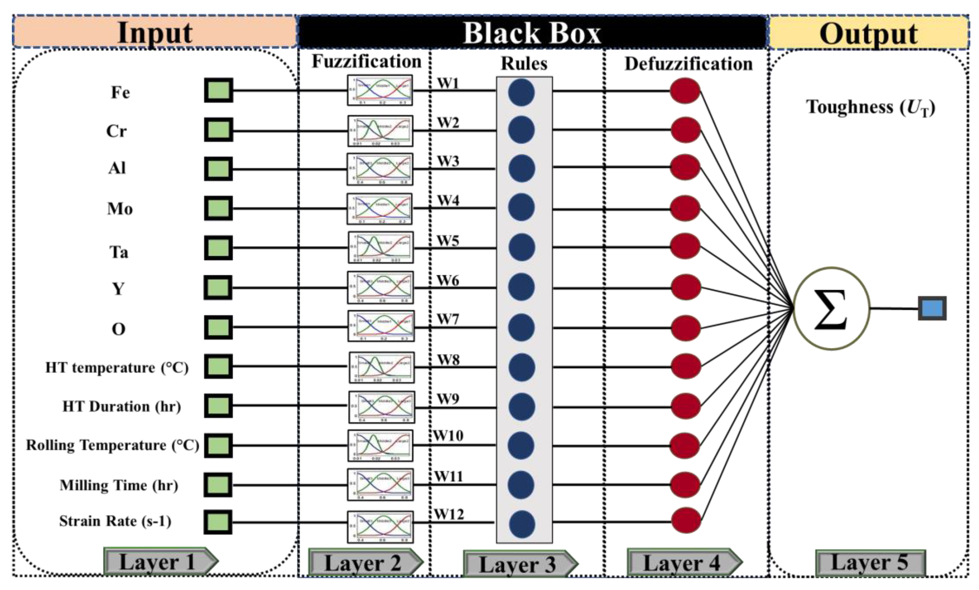
3. Machine Learning Methods Procedure
3.1. Artificial Neural Network (ANN)
3.2. Adaptive Neuro-Fuzzy Inference Systems (ANIFS)
3.3. Support Vector Regression (SVR)
4. Results and Discussion
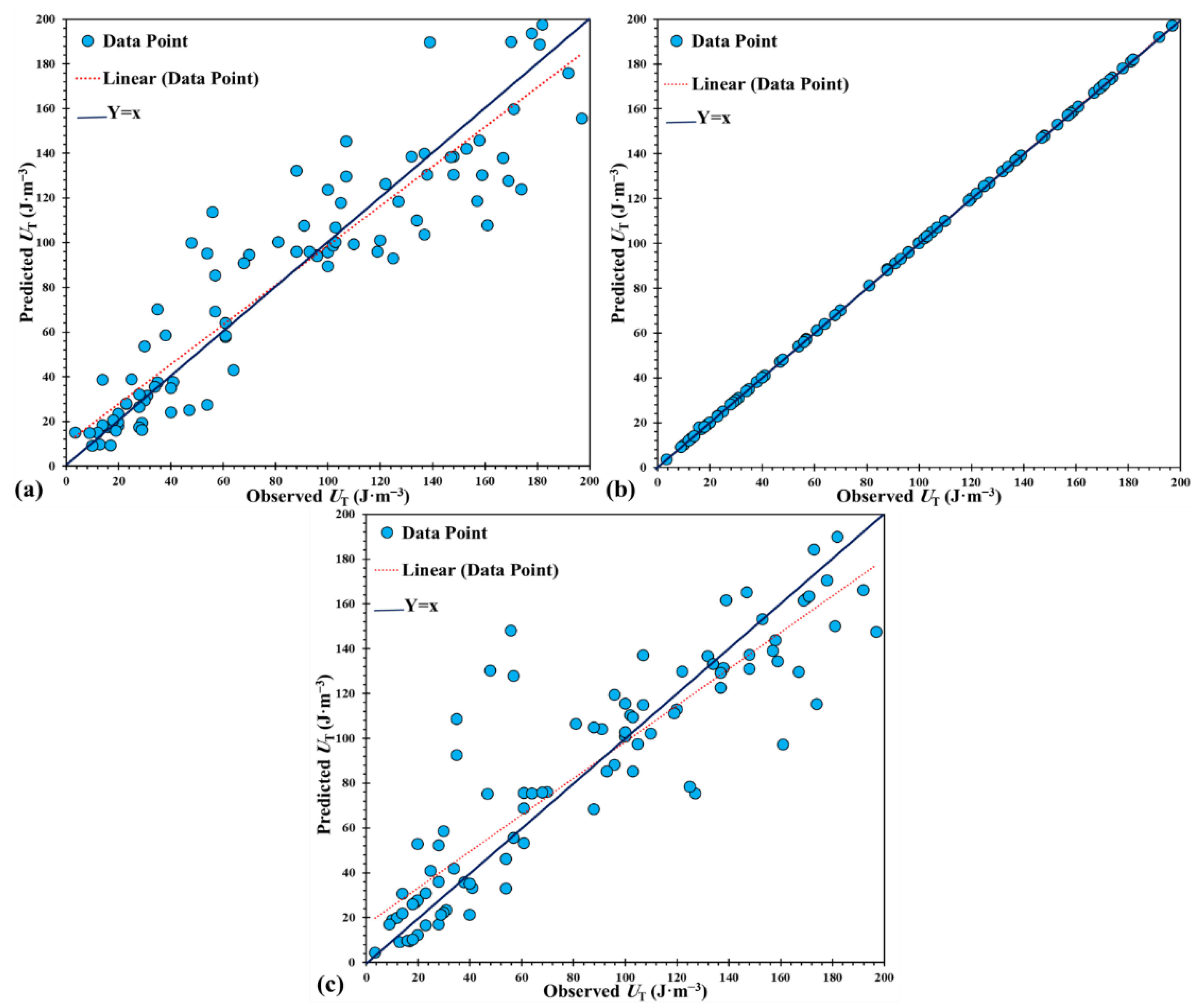
4.1. The Analysis of the Constructed Models
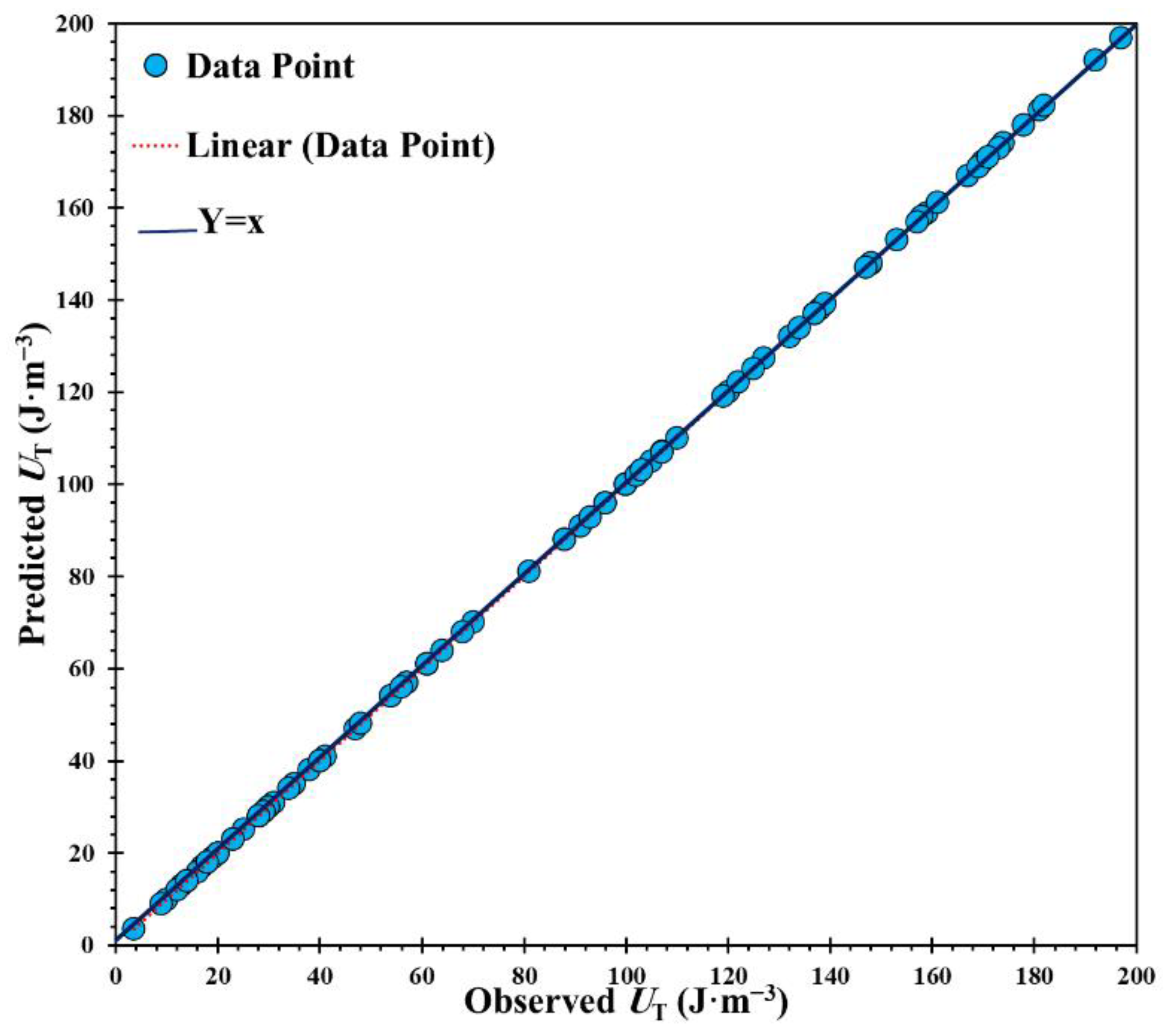
4.2. Analysis of the Validity and Performance of the Constructed Models
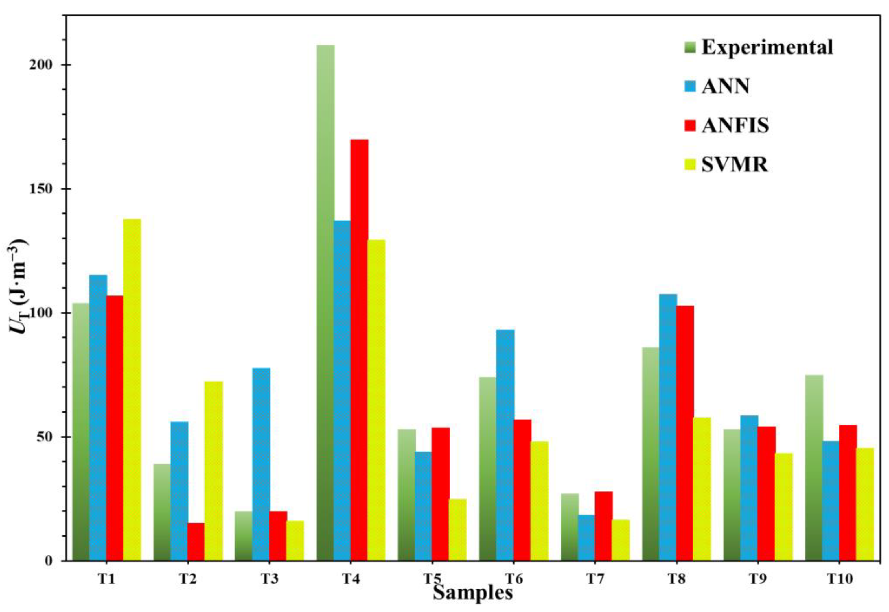
4.3. Prediction of the Toughness of OPH Alloys
4.4. Sensitivity Analysis (SA) of Input Parameters
5. Conclusions
Author Contributions
Funding
Institutional Review Board Statement
Informed Consent Statement
Data Availability Statement
Conflicts of Interest
References
- Oñoro, M.; Macías-Delgado, J.; Auger, M.; de Castro, V.; Leguey, T. Mechanical properties and stability of precipitates of an ODS steel after thermal cycling and aging. Nucl. Mater. Energy 2020, 24, 100758. [Google Scholar] [CrossRef]
- Zhao, H.; Liu, T.; Bai, Z.; Wang, L.; Gao, W.; Zhang, L. Corrosion behaviour of 14Cr ODS steel in supercritical water: The influence of substituting Y2O3 with Y2Ti2O7 nanoparticles. Corros. Sci. 2020, 163, 108272. [Google Scholar] [CrossRef]
- Kang, Z.; Shen, H.; Bai, Z.; Zhao, H.; Liu, T. Influences of different hydride nanoparticles on microstructure and mechanical properties of 14Cr3Al ferritic ODS steels. Powder Technol. 2019, 343, 137–144. [Google Scholar] [CrossRef]
- Wang, L.; Bai, Z.; Shen, H.; Wang, C.; Liu, T. Creation of Y2Ti2O7 nanoprecipitates to strengthen the Fe-14Cr-3Al-2W steels by adding Ti hydride and Y2O3 nanoparticles. J. Nucl. Mater. 2017, 488, 319–327. [Google Scholar] [CrossRef]
- Khalaj, O.; Saebnoori, E.; Jirková, H.; Chocholatý, O.; Svoboda, J. High Temperature and Corrosion Properties of A Newly Developed Fe-Al-O Based OPH Alloy. Metals 2020, 10, 167. [Google Scholar] [CrossRef] [Green Version]
- Zhao, Q.; Yu, L.; Liu, Y.; Li, H. Morphology and structure evolution of Y2O3 nanoparticles in ODS steel powders during mechanical alloying and annealing. Adv. Powder Technol. 2015, 26, 1578–1582. [Google Scholar] [CrossRef]
- Xu, H.; Lu, Z.; Wang, D.; Liu, C. Effect of zirconium addition on the microstructure and mechanical properties of 15Cr-ODS ferritic Steels consolidated by hot isostatic pressing. Fusion Eng. Des. 2017, 114, 33–39. [Google Scholar] [CrossRef]
- Zhang, L.; Yu, L.; Liu, Y.; Liu, C.; Li, H.; Wu, J. Influence of Zr addition on the microstructures and mechanical properties of 14Cr ODS steels. Mater. Sci. Eng. A 2017, 695, 66–73. [Google Scholar] [CrossRef]
- Parida, P.K.; Dasgupta, A.; Jayasankar, K.; Kamruddin, M.; Saroja, S. Structural studies of Y2O3 dispersoids during mechanical milling and annealing in a Fe-15 Y2O3 model ODS alloy. J. Nucl. Mater. 2013, 441, 331–336. [Google Scholar] [CrossRef]
- Brocq, M.; Radiguet, B.; Le Breton, J.-M.; Cuvilly, F.; Pareige, P.; Legendre, F. Nanoscale characterisation and clustering mechanism in an Fe-Y2O3 model ODS alloy processed by reactive ball milling and annealing. Acta Mater. 2010, 58, 1806–1814. [Google Scholar] [CrossRef]
- Khalaj, O.; Jirková, H.; Janda, T.; Kučerová, L.; Studený, T.; Svoboda, J. Improving the high-temperature properties of a new generation of Fe-Al-O oxide-precipitation-hardened steels. Mater. Technol. 2019, 53, 495–504. [Google Scholar] [CrossRef]
- Parida, P.K.; Dasgupta, A.; Raghavendra, K.; Jayasankar, K.; Saroja, S. Structural Studies of Dispersoids in Fe–15 wt% Y2O3–5 wt% Ti Model ODS Alloys During Milling and Subsequent Annealing. Trans. Indian Inst. Met. 2017, 70, 1409–1415. [Google Scholar] [CrossRef]
- Khalaj, O.; Jirková, H.; Masek, B.; Hassasroudsari, P.; Studecký, T.; Svoboda, J. Using thermomechanical treatments to improve the grain growth of new-generation ODS alloys. Mater. Technol. 2018, 52, 475–482. [Google Scholar] [CrossRef]
- Khalaj, O.; Jirková, H.; Burdová, K.; Stehlík, A.; Kučerová, L.; Vrtáček, J.; Svoboda, J. Hot Rolling vs. Forging: Newly Developed Fe-Al-O Based OPH Alloy. Metals 2021, 11, 228. [Google Scholar] [CrossRef]
- Khalaj, O.; Saebnoori, E.; Jirková, H.; Chocholatý, O.; Kučerová, L.; Hajšman, J.; Svoboda, J. The Effect of Heat Treatment on the Tribological Properties and Room Temperature Corrosion Behaviour of Fe–Cr–Al-Based OPH Alloy. Materials 2020, 13, 5465. [Google Scholar] [CrossRef] [PubMed]
- Khalaj, O.; Masek, B.; Jirková, H.; Bublíková, D.; Svoboda, J. Influence of thermomechanical treatment on the grain-growth behaviour of new Fe-Al based alloys with fine Al2O3 precipitates. Materiali in tehnologije 2017, 51, 759–768. [Google Scholar] [CrossRef]
- Masek, B.; Khalaj, O.; Novy, Z.; Kubina, T.; Jirkova, H.; Svoboda, J.; Stadler, C. Behaviour of new ODS alloys under single and multiple deformation. Mater. Technol. 2016, 50, 891–898. [Google Scholar] [CrossRef]
- Golafshani, E.M.; Behnood, A.; Arashpour, M. Predicting the compressive strength of normal and High-Performance Concretes using ANN and ANFIS hybridized with Grey Wolf Optimizer. Constr. Build. Mater. 2020, 232, 117266. [Google Scholar] [CrossRef]
- Akhtari-Goshayeshi, A.; Ghobadi, M.; Saebnoori, E.; Zarezadeh, A.; Rostami, M.; Nematollahi, M. Prediction of Corrosion Rate for Carbon Steel in Soil Environment by Artificial Neural Network and Genetic Algorithm. J. Adv. Mater. Process. 2019, 7, 29–38. [Google Scholar]
- Gupta, T.; Patel, K.; Siddique, S.; Sharma, R.K.; Chaudhary, S. Prediction of mechanical properties of rubberised concrete exposed to elevated temperature using ANN. Measurement 2019, 147, 106870. [Google Scholar] [CrossRef]
- Hernández-Julio, Y.F.; Prieto-Guevara, M.J.; Nieto-Bernal, W. Fuzzy clustering and dynamic tables for knowledge discovery and decision-making: Analysis of the reproductive performance of the marine copepod Cyclopina sp. Aquaculture 2020, 523, 735183. [Google Scholar] [CrossRef]
- Hosseinzadeh, A.; Zhou, J.L.; Altaee, A.; Baziar, M.; Li, X. Modelling water flux in osmotic membrane bioreactor by adaptive network-based fuzzy inference system and artificial neural network. Bioresour. Technol. 2020, 310, 123391. [Google Scholar] [CrossRef] [PubMed]
- Ghobadi, M.; Zaarei, D.; Naderi, R.; Asadi, N.; Seyedi, S.R.; Avard, M.R. Improvement the protection performance of lanolin based temporary coating using benzotriazole and cerium (III) nitrate: Combined experimental and computational analysis. Prog. Org. Coat. 2021, 151, 106085. [Google Scholar] [CrossRef]
- Jajarmi, E.; Sajjadi, S.A.; Mohebbi, J. Predicting the relative density and hardness of 3YPSZ/316L composites using adaptive neuro-fuzzy inference system and support vector regression models. Measurement 2019, 145, 472–479. [Google Scholar] [CrossRef]
- Xiong, J.; Shi, S.-Q.; Zhang, T.-Y. Machine learning of phases and mechanical properties in complex concentrated alloys. J. Mater. Sci. Technol. 2021, 87, 133–142. [Google Scholar] [CrossRef]
- Liu, G.; Jia, L.; Kong, B.; Feng, S.; Zhang, H.; Zhang, H. Artificial neural network application to microstructure design of Nb-Si alloy to improve ultimate tensile strength. Mater. Sci. Eng. A 2017, 707, 452–458. [Google Scholar] [CrossRef]
- Wu, J.; Huang, Z.; Qiao, H.; Zhao, Y.; Li, J.; Zhao, J. Artificial neural network approach for mechanical properties prediction of TC4 titanium alloy treated by laser shock processing. Opt. Laser Technol. 2021, 143, 107385. [Google Scholar] [CrossRef]
- Zhang, L.; Qian, K.; Huang, J.; Liu, M.; Shibuta, Y. Molecular dynamics simulation and machine learning of mechanical response in non-equiatomic FeCrNiCoMn high entropy alloy. J. Mater. Res. Technol. 2021, 232, 117266. [Google Scholar]
- Durodola, J. Machine learning for design, phase transformation and mechanical properties of alloys. Prog. Mater. Sci. 2021, 123, 100797. [Google Scholar] [CrossRef]
- Krishna, Y.V.; Jaiswal, U.K.; Rahul, M. Machine learning approach to predict new multiphase high entropy alloys. Scr. Mater. 2021, 197, 113804. [Google Scholar] [CrossRef]
- Li, M.; Mesbah, M.; Fallahpour, A.; Nasiri-Tabrizi, B.; Liu, B. Mechanical strength estimation of ultrafine-grained magnesium implant by neural-based predictive machine learning. Mater. Lett. 2021, 305, 130627. [Google Scholar] [CrossRef]
- Badmos, A.; Bhadeshia, H.; MacKay, D. Tensile properties of mechanically alloyed oxide dispersion strengthened iron alloys Part 1-Neural networkmodels. Mater. Sci. Technol. 1998, 14, 793–809. [Google Scholar] [CrossRef]
- Khalaj, O.; Ghobadi, M.; Zarezadeh, A.; Saebnoori, E.; Jirková, H.; Chocholaty, O.; Svoboda, J. Potential role of machine learning techniques for modelling the hardness of OPH steels. Mater. Today Commun. 2021, 26, 101806. [Google Scholar] [CrossRef]
- Kumar, D.; Prakash, U.; Dabhade, V.V.; Laha, K.; Sakthivel, T. High yttria ferritic ODS steels through powder forging. J. Nucl. Mater. 2017, 488, 75–82. [Google Scholar] [CrossRef]
- Franco, D.S.; Duarte, F.A.; Salau, N.P.G.; Dotto, G.L. Analysis of indium (III) adsorption from leachates of LCD screens using artificial neural networks (ANN) and adaptive neuro-fuzzy inference systems (ANIFS). J. Hazard. Mater. 2020, 384, 121137. [Google Scholar] [CrossRef] [PubMed]
- Zhou, Q.; Wang, F.; Zhu, F. Estimation of compressive strength of hollow concrete masonry prisms using artificial neural networks and adaptive neuro-fuzzy inference systems. Constr. Build. Mater. 2016, 125, 417–426. [Google Scholar] [CrossRef]
- Xu, J.; Zhao, X.; Yu, Y.; Xie, T.; Yang, G.; Xue, J. Parametric sensitivity analysis and modelling of mechanical properties of normal-and high-strength recycled aggregate concrete using grey theory, multiple nonlinear regression and artificial neural networks. Constr. Build. Mater. 2019, 211, 479–491. [Google Scholar] [CrossRef]
- Sugeno, M.; Kang, G. Structure identification of fuzzy model. Fuzzy Sets and Systems 1988, 28, 15–33. [Google Scholar] [CrossRef]
- Akkaya, E. ANFIS based prediction model for biomass heating value using proximate analysis components. Fuel 2016, 180, 687–693. [Google Scholar] [CrossRef]
- Cakmakci, M. Adaptive neuro-fuzzy modelling of anaerobic digestion of primary sedimentation sludge. Bioprocess Biosystems Eng. 2007, 30, 349–357. [Google Scholar] [CrossRef]
- Alrashed, A.A.; Gharibdousti, M.S.; Goodarzi, M.; de Oliveira, L.R.; Safaei, M.R.; Bandarra Filho, E.P. Effects on thermophysical properties of carbon based nanofluids: Experimental data, modelling using regression, ANFIS and ANN. Int. J. Heat Mass Transf. 2018, 125, 920–932. [Google Scholar] [CrossRef]
- Thissen, U.; Pepers, M.; Üstün, B.; Melssen, W.; Buydens, L. Comparing support vector machines to PLS for spectral regression applications. Chemom. Intell. Lab. Syst. 2004, 73, 169–179. [Google Scholar] [CrossRef]
- Smith, G.N. Probability and Statistics in Civil Engineering; Nichols Publishing Company: New York, NY, USA, 1986. [Google Scholar]
- Gandomi, A.H.; Mohammadzadeh, D.; Pérez-Ordóñez, J.L.; Alavi, A.H. Linear genetic programming for shear strength prediction of reinforced concrete beams without stirrups. Appl. Soft Comput. 2014, 19, 112–120. [Google Scholar] [CrossRef]
- Roy, P.P.; Roy, K. On some aspects of variable selection for partial least squares regression models. QSA Comb. Sci. 2008, 27, 302–313. [Google Scholar] [CrossRef]
- Tavana, M.; Fallahpour, A.; Di Caprio, D.; Santos-Arteaga, F.J. A hybrid intelligent fuzzy predictive model with simulation for supplier evaluation and selection. Expert Syst. Appl. 2016, 61, 129–144. [Google Scholar] [CrossRef]
- Tenza-Abril, A.J.; Villacampa, Y.; Solak, A.M.; Baeza-Brotons, F. Prediction and sensitivity analysis of compressive strength in segregated lightweight concrete based on artificial neural network using ultrasonic pulse velocity. Constr. Build. Mater. 2018, 189, 1173–1183. [Google Scholar] [CrossRef]
- Ibrahim, S.; Choong, C.E.; El-Shafie, A. Sensitivity analysis of artificial neural networks for just-suspension speed prediction in solid-liquid mixing systems: Performance comparison of MLPNN and RBFNN. Adv. Eng. Inform. 2019, 39, 278–291. [Google Scholar] [CrossRef]
- Yaïci, W.; Longo, M.; Entchev, E.; Foiadelli, F. Simulation study on the effect of reduced inputs of artificial neural networks on the predictive performance of the solar energy system. Sustainability 2017, 9, 1382. [Google Scholar] [CrossRef] [Green Version]
- Pasini, A. Artificial neural networks for small dataset analysis. J. Thorac. Dis. 2015, 7, 953. [Google Scholar]


| Variable | Unit | Range |
|---|---|---|
| Fe | wt % | 0.7106–0.8743 |
| Cr | wt % | 0–0.1533 |
| Al | wt % | 0.0032−0.1093 |
| Mo | wt % | 0–0.0383 |
| Ta | wt % | 0–0.0083 |
| Y | wt % | 0–0.0364 |
| O | wt % | 0–0.0098 |
| Milling time | hours | 150–480 |
| Rolling Temperature | °C | 850–960 |
| HT duration | hours | 0–20 |
| HT temperature | °C | 25–1200 |
| Strain Rate | s−1 | 0.001–10 |
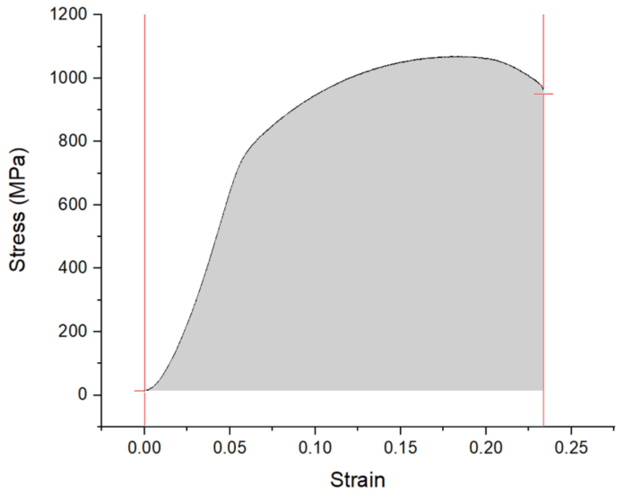
| Toughness | J·m−3 | 3.5–208 |
| ANN Models | Training Algorithm | Symbol | MSE | MAE | R2 |
|---|---|---|---|---|---|
| ANN-1 | Resilient backpropagation | RP | 776.65 | 20.85 | 0.76 |
| ANN-2 | BFGS quasi-Newton backpropagation | BFG | 785.53 | 20.37 | 0.75 |
| ANN-3 | Scaled Conjugate Gradient | SCG | 812.58 | 22.65 | 0.67 |
| ANN-4 | Levenberg–Marquardt backpropagation | LM | 459.22 | 15.75 | 0.86 |
| ANN-5 | Conjugate Gradient with Powell/Beale Restarts | CGB | 876.25 | 27.47 | 0.60 |
| ANFIS Models | RI | SF | The Number of Input MF | Number of Rules | Epochs | RMSE |
|---|---|---|---|---|---|---|
| ANFIS-SC1 | 1 | 2 | 6 | 6 | 20 | 38.49 |
| ANFIS-SC2 | 0.9 | 1.5 | 11 | 11 | 40 | 262.48 |
| ANFIS-SC3 | 0.8 | 3 | 4 | 4 | 60 | 32.68 |
| ANFIS-SC4 | 0.7 | 1.75 | 14 | 14 | 80 | 29.41 |
| ANFIS-SC5 | 0.6 | 2.5 | 11 | 11 | 50 | 71.36 |
| ANFIS-SC6 | 0.5 | 1.25 | 30 | 30 | 30 | 10.35 |
| ANFIS-SC7 | 0.4 | 2.25 | 26 | 26 | 70 | 14.56 |
| ANFIS-SC8 | 0.3 | 1 | 61 | 61 | 100 | 0.20 |
| ANFIS-SC9 | 0.2 | 6 | 26 | 26 | 90 | 56.55 |
| ANFIS-SC10 | 0.1 | 7 | 48 | 48 | 15 | 6.44 |
| Item | Formula | Condition | ANN | ANFIS | SVR |
|---|---|---|---|---|---|
| 1 | R = | 0.8 < R | 0.926 | 0.999 | 0.892 |
| 2 | k = | 0.85 < k < 1.15 | 0.969 | 1.0001 | 0.953 |
| 3 | k′ = | 0.85 < k′ < 1.15 | 0.986 | 0.999 | 0.983 |
| 4 | = 1 − , = k × ti | 1 | 0.997 | 0.999 | 0.992 |
| 5 | = 1 − , = k′ × hi | 1 | 0.999 | 0.999 | 0.999 |
| Material No. | Milling Time (h) | Rolling Temp. (°C) | Annealing | Strain Rate (S−1) | Chemical Composition (wt %) | Experimental UT (J·m−3) | Predicted UT (J·m−3) | ||
|---|---|---|---|---|---|---|---|---|---|
| ANN (R2 = 0.60) | ANFIS (R2 = 0.88) | SVR (R2 = 0.55) | |||||||
| T1 | 150 | 925 | 1200 °C-1 h | 0.1 | 1250 gZ + 90 gAl + 40 gY2O3 + 50Mo + 12Ta, Z = 83Fe + 17Cr | 104 | 115.2745 | 106.9551 | 137.825 |
| T2 | 230 | 925 | 1200 °C-5 h | 0.001 | 1500 gZ + 108 gAl + 70 gY2O3 + 60Mo + 14Ta, Z = 83Fe + 17Cr | 39 | 55.9562 | 15.27325 | 72.43799 |
| T3 | 230 | 925 | 1000 °C-5 h | 10 | 1500 gZ + 108 gAl + 70 gY2O3 + 60Mo + 14Ta, Z = 83Fe + 17Cr | 20 | 77.6837 | 19.93451 | 16.01895 |
| T4 | 480 | 960 | 1100 °C-5 h | 0.001 | 800Fe + 100Al + 30Y2O3 + 7Y | 208 | 137.1719 | 169.7749 | 129.4625 |
| T5 | 480 | 960 | 1000 °C-20 h | 0.001 | 800Fe + 100Al + 15O2 | 53 | 44.1085 | 53.7416 | 24.93518 |
| T6 | 230 | 850 | 1000 °C-20 h | 0.001 | 400 gFe + 80 gCr + 36 gAl + 20 gY2O3 | 74 | 93.2575 | 56.98798 | 48.08971 |
| T7 | 230 | 865 | 800 °C-1 h | 0.1 | 1200 gFe + 240 gCr + 108 gAl + 75 gY2O3 | 27 | 18.5657 | 27.99824 | 16.53388 |
| T8 | 230 | 865 | 1100 °C-20 h | 0.1 | 1200 gFe + 240 gCr + 108 gAl + 75 gY2O3 | 86 | 107.5968 | 102.7684 | 57.76867 |
| T9 | 230 | 873 | 800 °C-5 h | 0.1 | 2400 gFe + 480 gCr + 216 gAl + 120 gY2O3 + 120Mo | 53 | 58.5657 | 54.1952 | 43.41673 |
| T10 | 230 | 860 | 800 °C-1 h | 0.001 | 2400 gFe + 480 gCr + 216 gAl + 120 gY2O3 + 120Mo | 75 | 48.3064 | 54.646 | 45.41388 |
| No. | ANFIS Model | R2 | MSE | MAE |
|---|---|---|---|---|
| 1 | 11 Input Parameters | 0.9999868 | 0.0417606 | 0.0517638 |
| 2 | 10 Input Parameters (without Fe) | 0.9999917 | 0.0261573 | 0.0442478 |
| 3 | 10 Input Parameters (without Cr) | 0.9999994 | 0.0017188 | 0.0186334 |
| 4 | 10 Input Parameters (without Al) | 0.9968289 | 10.1001732 | 0.4402436 |
| 5 | 10 Input Parameters (without Mo) | 0.9927615 | 23.0551972 | 1.4600404 |
| 6 | 10 Input Parameters (without Ta) | 0.9505068 | 157.6411613 | 2.0653843 |
| 7 | 10 Input Parameters (without Y) | 0.9999796 | 0.0648635 | 0.1063068 |
| 8 | 10 Input Parameters (without O) | 0.9948345 | 16.4525800 | 0.5791974 |
| 9 | 10 Input Parameters (without Milling time) | 0.9950622 | 15.7271643 | 1.1247957 |
| 10 | 10 Input Parameters (without Rolling Temperature) | 0.9678562 | 102.3813008 | 3.1022166 |
| 11 | 10 Input Parameters (without HT temperature) | 0.5434395 | 1454.195369 | 27.4952115 |
| 12 | 10 Input Parameters (without HT duration) | 0.8766828 | 392.7787824 | 13.4959577 |
| 13 | 10 Input Parameters (without Strain rate) | 0.9810307 | 60.4190996 | 3.2876585 |
| Error | R2 | MSE | MAE | |
|---|---|---|---|---|
| Model | ||||
| ANFIS | 0.9999868 | 0.0417606 | 0.0517638 | |
| Optimized ANFIS | 0.9999988 | 0.0039412 | 0.0299045 | |
Publisher’s Note: MDPI stays neutral with regard to jurisdictional claims in published maps and institutional affiliations. |
© 2021 by the authors. Licensee MDPI, Basel, Switzerland. This article is an open access article distributed under the terms and conditions of the Creative Commons Attribution (CC BY) license (https://creativecommons.org/licenses/by/4.0/).
Share and Cite
Khalaj, O.; Ghobadi, M.; Saebnoori, E.; Zarezadeh, A.; Shishesaz, M.; Mašek, B.; Štadler, C.; Svoboda, J. Development of Machine Learning Models to Evaluate the Toughness of OPH Alloys. Materials 2021, 14, 6713. https://doi.org/10.3390/ma14216713
Khalaj O, Ghobadi M, Saebnoori E, Zarezadeh A, Shishesaz M, Mašek B, Štadler C, Svoboda J. Development of Machine Learning Models to Evaluate the Toughness of OPH Alloys. Materials. 2021; 14(21):6713. https://doi.org/10.3390/ma14216713
Chicago/Turabian StyleKhalaj, Omid, Moslem Ghobadi, Ehsan Saebnoori, Alireza Zarezadeh, Mohammadreza Shishesaz, Bohuslav Mašek, Ctibor Štadler, and Jiří Svoboda. 2021. "Development of Machine Learning Models to Evaluate the Toughness of OPH Alloys" Materials 14, no. 21: 6713. https://doi.org/10.3390/ma14216713