Article

Advanced Computational Fluid Dynamics Study of the Dissolved Oxygen Concentration within a Thin-Layer Cascade Reactor for Microalgae Cultivation

by
Karel Petera
1,*,
Štěpán Papáček
2,
Cristian Inostroza González
3,
José María Fernández-Sevilla
3 and
Francisco Gabriel Acién Fernández
3
1
Department of Process Engineering, Faculty of Mechanical Engineering, Czech Technical University in Prague, Technická 4, 16000 Prague, Czech Republic
2
The Czech Academy of Sciences, Institute of Information Theory and Automation, Pod vodárenskou věží 4, 18000 Prague, Czech Republic
3
Chemical Engineering Department, University of Almería, Ctra. Sacramento s/n La Cañada de San Urbano, 04120 Almería, Spain
*
Author to whom correspondence should be addressed.
Energies 2021, 14(21), 7284; https://doi.org/10.3390/en14217284
Submission received: 3 October 2021 / Revised: 25 October 2021 / Accepted: 30 October 2021 / Published: 3 November 2021
(This article belongs to the Special Issue Modeling, Optimization and Control in Algal Biotechnology)

Abstract

:
High concentration of dissolved oxygen within microalgae cultures reduces the performance of corresponding microalgae cultivation system (MCS). The main aim of this study is to provide a reliable computational fluid dynamics (CFD)-based methodology enabling to simulate two relevant phenomena governing the distribution of dissolved oxygen within MCS: (i) mass transfer through the liquid–air interface and (ii) oxygen evolution due to microalgae photosynthesis including the inhibition by the same dissolved oxygen. On an open thin-layer cascade (TLC) reactor, a benchmark numerical study to assess the oxygen distribution was conducted. While the mass transfer phenomenon is embedded within CFD code ANSYS Fluent, the oxygen evolution rate has to be implemented via user-defined function (UDF). To validate our methodology, experimental data for dissolved oxygen distribution within the 80 meter long open thin-layer cascade reactor are compared against numerical results. Moreover, the consistency of numerical results with theoretical expectations has been shown on the newly derived differential equation describing the balance of dissolved oxygen along the longitudinal direction of TLC. We argue that employing our methodology, the dissolved oxygen distribution within any MCS can be reliably determined in silico, and eventually optimized or/and controlled.

1. Introduction

First-generation biofuels were an interesting alternative to provide energy for the automotive and air travel sectors but its reliance on edible feedstocks undermined their viability. Although it is technically possible to obtain biofuels from microalgae, commercial production is still not possible due to economic and other limiting factors, but the scientific community did not lose interest in working with these simple photosynthetic microorganisms such as cyanobacteria and microalgae [1]. These incredibly versatile microorganisms have been attracting much research interest for more than half a century, mainly for high photosynthetic efficiency, biomass growth, and lipid content [2]. Microalgae are oxygenic unicellular phototrophs, which utilize light energy to fix inorganic carbon (CO 2 ) to synthetize more complex organic molecules in photosynthetic reactions. Moreover, they produce oxygen but also consume inorganic nitrogen and phosphorus, thus may participate in wastewater treatment processes [2,3].
However, there are two limiting factors or drawbacks for microalgae products commercialization: (i) the high costs of microalgae biomass production in microalgae culture systems (MCS), e.g., photobioreactors (PBRs), and (ii) lack of reliable mathematical models for further in silico optimization of the whole production process. Leaving apart the first point, we would rather dedicate our efforts to overcome the second one. The complexity of mathematical modeling of MCS resides in the fact that we deal with multiple physical and biological (inherently nonlinear) phenomena, e.g., three-dimensional multiphase (gas–liquid–solid) flow dynamics (with mass transfer through the air–liquid interface), irradiance distribution within the illuminated parts of MCS, and multi-level functionality of cellular processes. Moreover, all these parts, which have to be integrated with the corresponding PBR operation mode, interact across different timescales. Although there exist new measurement technologies and theoretical approaches, most studies of general MCS are focused on partial problems without clear interconnection, cf. [4,5]. Resuming, reliable methods with predictive power for in silico simulation of microbial growth in MCS are rather slowly emerging than being well established [6].
In this study, we present a solution of one specific yet cumbersome problem consisting in modeling and simulation of the dissolved oxygen distribution within a MCS, as far as we know, not yet resolved. It is well known that factors causing environmental stress act simultaneously [7]; here, we point out the high oxygen concentrations. It was reported that the dissolved oxygen concentration above values of 250% Sat. reduce the performance of microalgae cultures in closed photobioreactors [8,9] as well as open systems, i.e., thin-layer cascades [10,11] and raceways [12,13]. Recently, Kazbar et al. [14] used an improved kinetic growth model to explain the discrepancy in performance between two photobioreactor geometries. Furthermore, the authors of [14] proposed to control the gas–liquid mass transfer via aeration in order to enhance the photobioreactor performance. Moreover, Sousa et al. [15] reported that elevated oxygen concentrations do not contribute to photooxidative damage at the light conditions that are predominantly experienced by algae in closed photobioreactors, but only inhibit the growth via photorespiration effects. As Sforza et al. [9] stated: “Only a few quantitative approaches have attempted to describe and model oxygen inhibition, which is the result of different biological mechanisms.” In their study, they applied a photorespirometric protocol to assess and quantify the effect of high oxygen concentration on photosynthetic production rate, resulting in a new formula to describe the photosynthetic rate as a function of oxygen concentration. Let us underline, that our CFD-based methodology is independent on a particular oxygen inhibition model, i.e., any particular model can be implemented via user-defined function (UDF).
As follows, rather than propose a solution for a specific problem concerning microalgae cultivation within MCS, we present an advanced computational fluid dynamics (CFD) study of the dissolved oxygen concentration within a thin-layer cascade reactor for microalgae cultivation. The modeling framework integrating the fluid dynamics and photosynthetic oxygen evolution within CFD code is described in Section 2. In addition, a simplified description of the system in terms of an ordinary differential equation is presented there. Section 3 provides results and discussion of numerical simulations, illustration of mass transfer effects, and comparison with experimental data presented in illustrative figures, showing the consistency of numerical results with theoretical expectations. Finally, in Section 4, we draw some conclusions and future goals.

2. Materials and Methods

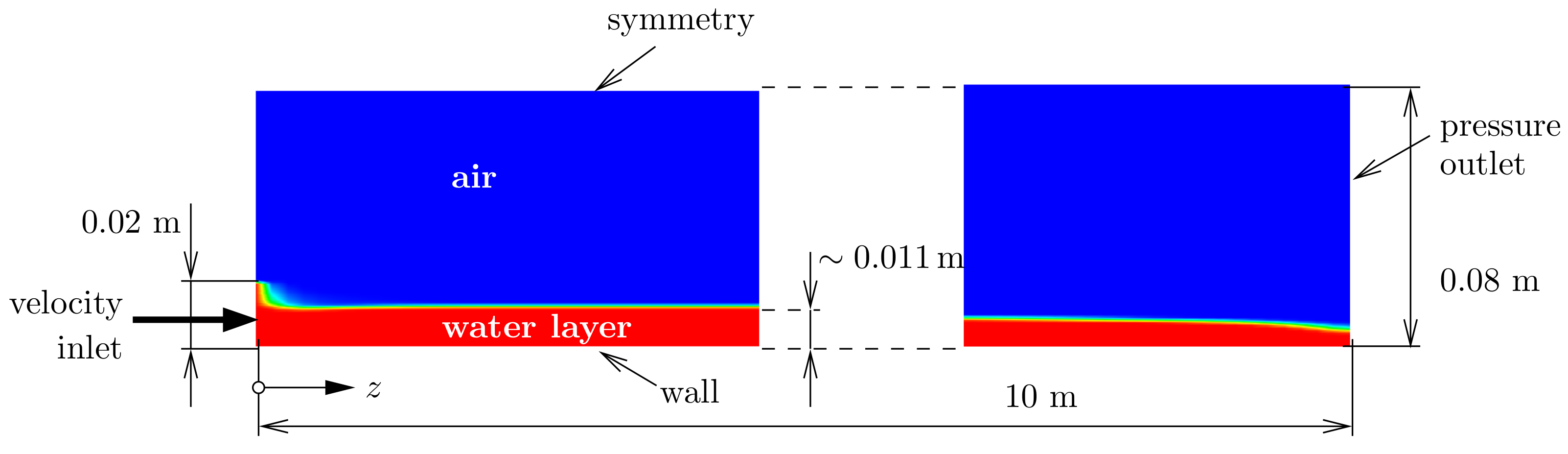
2.1. Thin-Layer Reactor Design and Operating Conditions

The first generation of the so-called thin-layer cascades (TLC) for microalgae production were developed at the end of the 1950s in former Czechoslovakia, see [16]. In this study, we used the experimental data measured on the TLC reactor located at the IFAPA Research Centre (Almería, Spain). This reactor consists of two sloped illuminated cultivation plates, each 40 m long and 1.5 m wide, connected by a flat channel. This reactor has a total volume of microalgae culture of 3.4 m 3 and is composed of three main parts: (a) two inclined channels with a solar radiation capture surface of 120 m 2 capable of containing 2.4 m 3 of culture with 0.02 m depth approximately, (b) tank or reservoir with 0.7 m 3 of culture, and (c) bubble column with 0.3 m 3 of culture with constant aeration which purpose is twofold: (i) to avoid the accumulation of dissolved oxygen, and (ii) to adjust the pH when necessary by the injection of CO 2 . TLC operation consists in circulating the microalgae culture by a hydraulic pump from the reservoir to the inclined channels, previously adjusting chemical parameters in the bubble column. Due to the area-volume ratio this type of reactors has a high photosynthetic efficiency and it worked in continuous production mode harvesting up to 1.0 m 3 /day (dilution ratio of 0.3/day), see [11] for details.
Based on the above operating conditions, the numerical model and corresponding boundary conditions have been set up, see Section 2.3.

2.2. Dissolved Oxygen Concentration within TLC and Its Impact on Photosynthetic Efficiency

The spatial inhomogeneity of culture conditions (average irradiance, temperature, pH, and dissolved oxygen) was found in different studies, see, e.g., in [10,11]. In this study, only the spatial variation of dissolved oxygen concentration is in the scope of our interest, and the microalgae strain Scenedesmus almeriensis (CCAP 276/24) is selected for its adaptability and abundant growth in outdoor reactors such as TLC. Barceló-Villalobos et al. [11] found that the dissolved oxygen concentration increased along the channel length due to photosynthetic oxygen evolution, see Figure 2D in [11]. The mean values of dissolved oxygen concentration ranged from 141 to 197% Sat (Table 1 in [11]), although values up to 225% Sat were experimentally determined.
As follows, the relations for the photosynthesis rate (depending on some parameters and the average irradiance only), as well as for the reduction of the photosynthetic efficiency due to the high dissolved oxygen concentration values, are important in the description of such systems. As a model for the photosynthesis rate, the hyperbolic model proposed in [17] is used:
PO 2 = PO 2 , max I av n I k n + I av n ,
and to quantify the reduction of photosynthetic efficiency, the same model as in [11] (adopted from [18,19]) is used:
PO 2 , inhib = PO 2 1 x O 2 x O 2 , max m .

2.3. CFD Model

2D rectangular geometry representing a cross section of the thin-layer photobioreactor was used in our CFD simulations. The length of the simulated system was 10 m and its height was 0.08 m. The system is slightly inclined, with a 1% slope which was reflected by a modified gravity vector g = ( 0.01 , 9.81 ) m s 2 in ANSYS Fluent. A structured mesh was created with the number of cells ~200 thousand. The Euler–Euler Multiphase model was used in ANSYS Fluent with Species Transport activated (the standard VOF multiphase model cannot be used with species transport simultaneously). Realizable variant of k ε turbulence model was used (with Enhanced Wall Treatment). In the first stage, only the momentum and volume fraction equations were solved to get developed velocity profile as well as the position of gas–liquid interface. Figure 1 illustrates the basic geometry including volume fraction contours and boundary conditions. The average thickness of the water layer developed along the bottom wall was ~11 mm; it decreases from the maximum 20 mm at the inlet to the minimum at the outlet 6 mm approximately.
To decrease the computational requirements in the next stage of simulations, the equations describing the momentum balance and volume fraction were not solved assuming that they will not change substantially, and only equations describing species transport and reaction were solved.

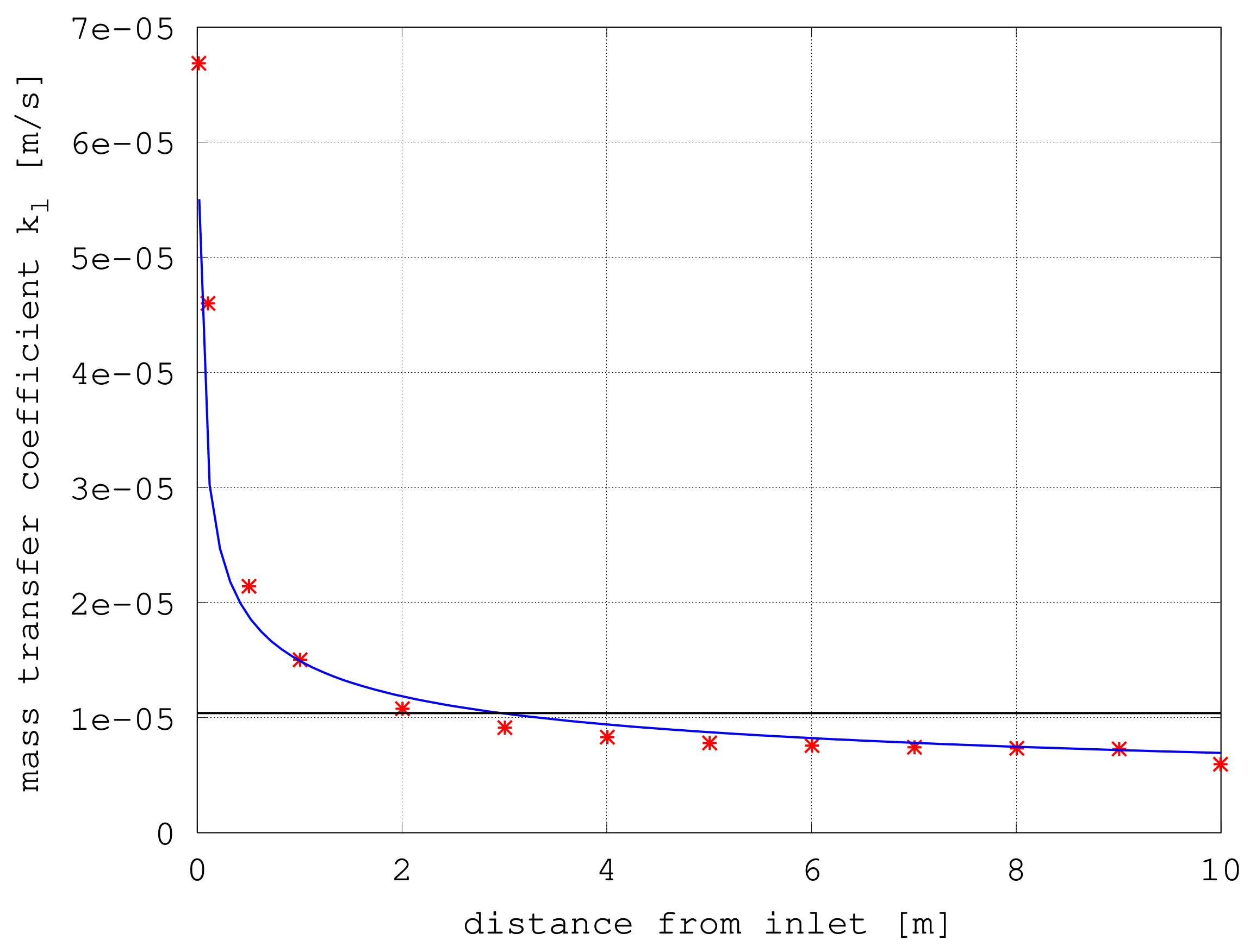
2.4. Mass Transfer across Gas–Liquid Interface

Mass transfer across the gas–liquid interface can be expressed using the mass transfer coefficients on both sides [20], in the liquid and in the gas phase. Their combination will give the overall mass transfer coefficient as
1 K L = 1 k l + 1 H O 2 k g .
H O 2 is Henry coefficient describing equilibrium between the concentration in the gas and liquid phases according to Henry’s law:
c G , O 2 = H O 2 c L , O 2 .
ANSYS Fluent has correlations describing the mass transfer coefficient but they are oriented to flow past spherical particles (bubbles) like Ranz–Marshall or Hugmark models [21]. These models are not suitable for this case of moving thin-water layer, therefore constant values of mass transfer coefficients were used instead. The gas side mass transfer coefficient was approximated using the correlation describing the flow along a flat plate as k g = 5.2 × 10 4 m s 1 . To determine the mass transfer coefficient on the liquid side, a separate CFD simulation describing the flow of the thin water layer with constant height was performed. In general, the mass transfer coefficient depends on the location, as it is illustrated in Figure 2.
At the locations near the the inlet, the values of the mass transfer coefficients are much larger than further from the inlet (theoretically, infinitely large for zero distance). The average value over the whole length (10 m in this case) was evaluated from an overall mass balance as k l = 1.02 × 10 5 m s 1 in this case, which corresponds to the experimental value already measured in [12]. Its value is much smaller than the gas-side coefficient, therefore the resistance to mass transfer is much larger in the liquid phase and we can safely assume that the overall mass transfer coefficient will be almost equal to the liquid-side mass transfer coefficient, that is, K L = k l . The dependency of the mass transfer coefficient (on the liquid side only) illustrated on Figure 2 could be described by the following equation:
k l = 1.5 × 10 5 z 1 / 3 [ m s 1 ] ,
where the asymptotic confidence interval of the leading constant is 8.7%. This equation could be then transformed into the correlation for the local value of the Sherwood number as
Sh z = k l z D O 2 = 0.243 Re z 2 / 3 Sc 1 / 3 , Re z = u z ν ,
where the distance from the inlet z is the characteristic length in both the Sherwood and Reynolds numbers. In general, the longer would be the system, the smaller dependency on the distance could be expected; thus, a constant average value would be a good approximation in such cases.

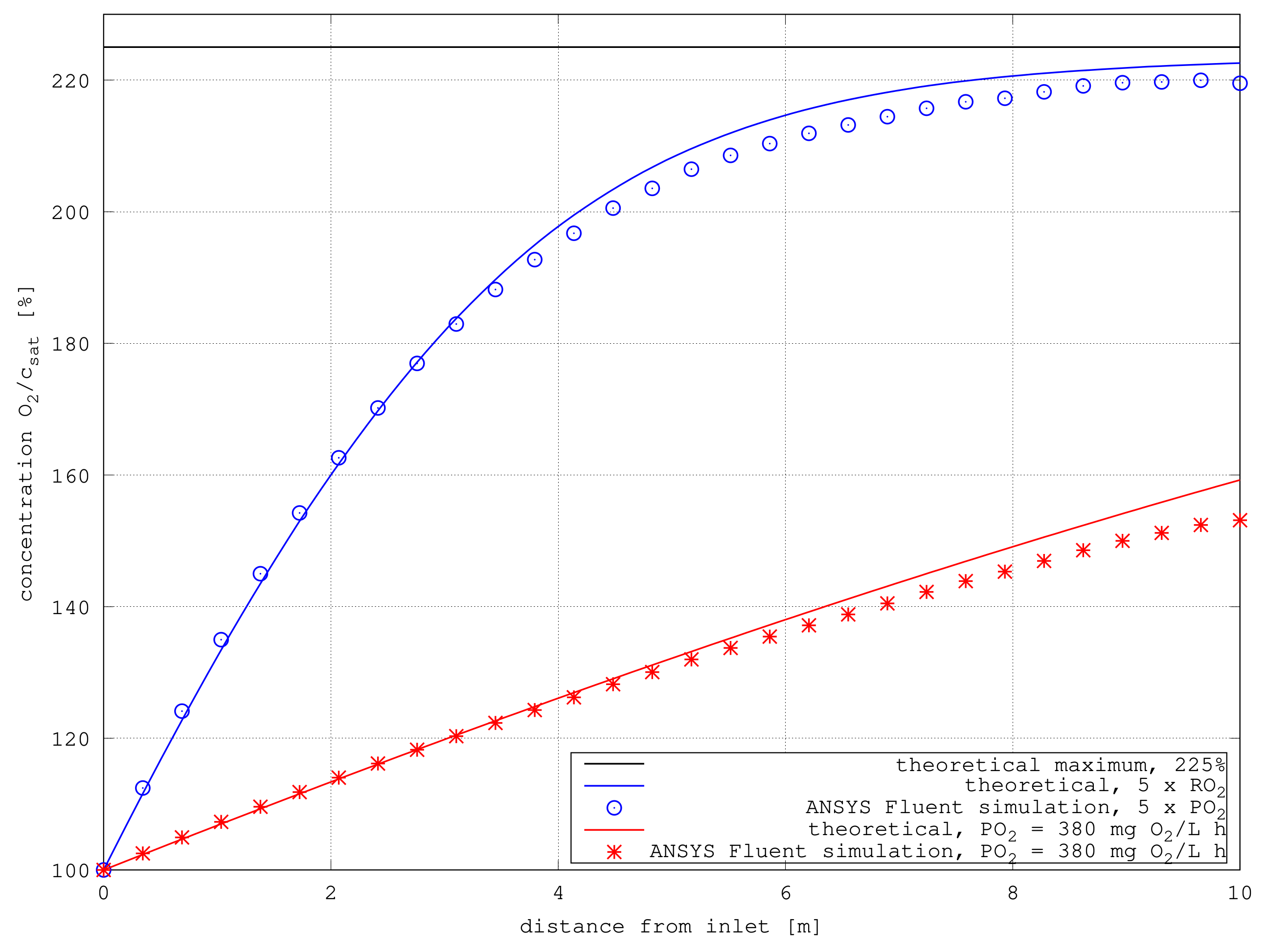
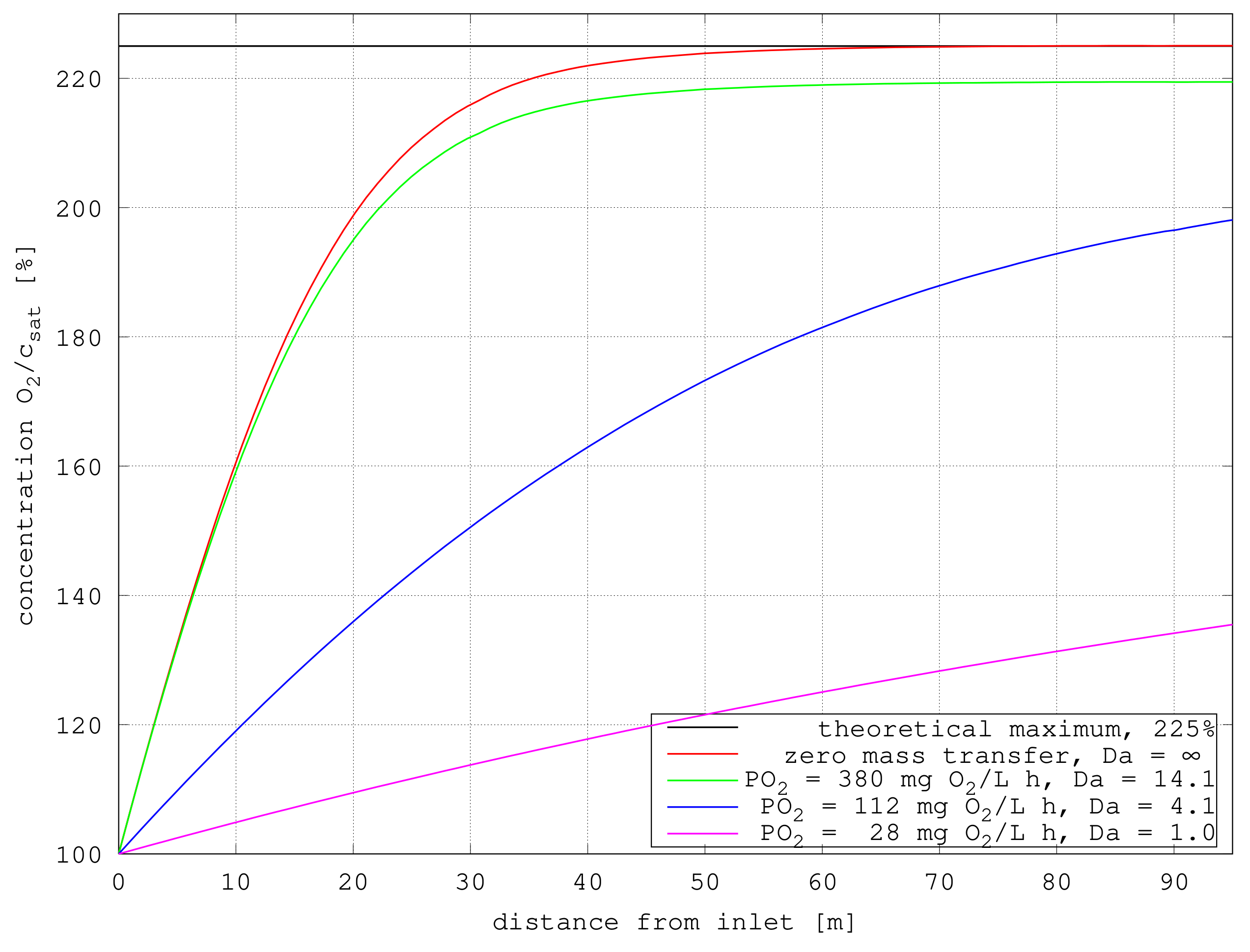
2.5. Simplified Description of Oxygen Concentration Profile

If we wanted to avoid time-consuming CFD simulations with this geometrical case of TLC reactor, we can simplify the thin water layer as a plug-flow system with constant velocity in the cross section. Then, it is possible to describe the concentration of dissolved oxygen along the length of the system (z-coordinate, see Figure 1) by the following differential equation:
N L d x O 2 d z = K L a c L , O 2 * x O 2 c L + PO 2 .
Here, N L is the molar flux of the liquid phase ( kmol m 2 s 1 ), x O 2 is molar fraction of dissolved oxygen, and c L , O 2 * is the corresponding concentration of oxygen in the gas phase transformed to equilibrium concentration in the liquid using Henry’s law (4) as c L , O 2 * = c G , O 2 / H O 2 . The term c L represents the total molar concentration of the liquid phase (it is close to the molar concentration of water as the amount of the dissolved oxygen is relatively small), and PO 2 is a reaction term representing the production of oxygen by microalgae cells. Term a in Equation (7) represents the specific surface of the interfacial area which can be derived from the ratio of differential element surface d A and its volume d V , i.e., d A d V , giving just reciprocal value of the liquid layer thickness a = 1 / h (h~11 mm in average for the developed layer, see Figure 1).
Reaction term PO 2 in Equation (7) can depend on various parameters, mainly the irradiation of the algae cells and corresponding rate of photosynthesis. The dependency on irradiance can be described by Equation (1) with parameters determined in [11] as PO 2 , max = 380 mg O 2 / L h , I k = 200 μ E / m 2 s , n = 2 . An average value of the irradiance I av is used, provided the sufficient mixing in TLC reactor, cf. [22]. Moreover, it was difficult to find a clear tendency describing the local values along the length of the reactor [11]. If the values of dissolved oxygen in the water are too large, they can inhibit the growth rate and photosynthesis, which was in our model described by Equation (2), where x O 2 , max , representing maximum concentration tolerated by the culture, was determined as 225% of saturated concentration along with parameter m = 3.5 [11]. Equation (1) along with (2) can be then used to replace the reaction term in Equation (7):
PO 2 = PO 2 , max I av n I k n + I av n 1 x O 2 x O 2 , max m
and reflect the inhibition by the dissolved oxygen in such way. For CFD simulations, this term was implemented in ANSYS Fluent through a user-defined function and DEFINE_VR_RATE macro. This equation provides the possibility to include also the dependency of the irradiance on the depth (or distance from the irradiated surface) using Beer–Lambert’s law, for example, see in [23] for an implementation of such dependency. Although the implementation of an irradiance model for local irradiance depending on the water depth does not represent neither theoretical nor computational difficulties, in this study, for the sake of clarity, based on the relatively small height of the water, we used the average irradiance value I av instead. Equations (7) and (8) represent a simplified description of the system which could be used to perform a parametric analysis of the whole system (with more complex geometries and flow patterns this would not be possible and CFD simulations would represent the only way in such cases).

3. Results and Discussion

3.1. CFD Simulations

ANSYS Fluent software package was used to perform CFD simulations in this work. A user-defined function (UDF) was implemented for the reaction term including the inhibition by dissolved oxygen (Equation (8)). Even though there would be a possibility to include also the spatial dependency of the irradiation according to the Beer–Lambert law, we operated here with constant irradiance getting us close to the maximum value PO 2 , max mentioned above ( 380 mg O 2 / L h recalculated as 3.3 × 10 6 kmol O 2 m 3 s 1 because these are units which must be used in ANSYS Fluent UDF).
At the inlet of the liquid phase, it was assumed that the concentration of the dissolved oxygen was equal to the saturated value, and the same value was used as the initial condition in the whole liquid domain. It was assumed to be constant even though it depends on temperature, in general. Concerning the gas phase as air, standard oxygen molar fraction was used (21%). A time-step analysis was performed according to the grid convergence index analysis [24], and the simulations describing the species transport including the reaction were finally performed with time step 0.01 s (developed velocity field and volume fraction were based on simulations with time step 0.001 s) which provided numerical accuracy expressed in terms of GCI below 1%. To get a steady-state representation of the concentration profiles along the reactor 10 m long, the total time of 100 s was simulated.
Figure 3 illustrates the concentration of dissolved oxygen along the almost horizontal line traced 5 mm from the bottom of the cultivation plate (that is, roughly in the middle of the thin liquid layer) for the standard value of the maximum reaction rate (see above) and 5 times larger which clearly approaches the maximum possible concentration representing 225% of the saturated value (depicted as a horizontal line at the top of the figure). The continuous lines in the figure represent the numerical solutions of ordinary differential Equation (7), and good agreement can be seen here.

3.2. Mass Transfer Effects

To assess the effect of mass transfer across the gas-liquid interface, we can focus on a steady-state balance of oxygen in the liquid phase, that is, on a situation with large length of the system where the derivative with respect to coordinate z in Equation (7) approaches zero:
0 = K L a c L x O 2 * x O 2 + PO 2 1 x O 2 x O 2 , max m .
After some manipulation, the previous equation can be transformed to the following form:
0 = 1 x O 2 x O 2 * + Da 1 x O 2 x O 2 , max m , Da = PO 2 K L a c L x O 2 * ,
where Da represents a variant of the Damköhler number, widely used in chemical engineering. Here, it represents the ratio of the reaction rate and mass transfer rate. The larger is the reaction rate compared to the mass transfer rate, that is, the larger is the value of the Damköhler number, the smaller is the impact of the mass transfer on the results, and vice versa. With zero mass transfer, that is Da , Equations (9) or (10) will result in concentration profile of dissolved oxygen approaching x O 2 , max . It is illustrated on Figure 4, where it is compared with other values of reaction (production) rate R O 2 and corresponding Damköhler number.

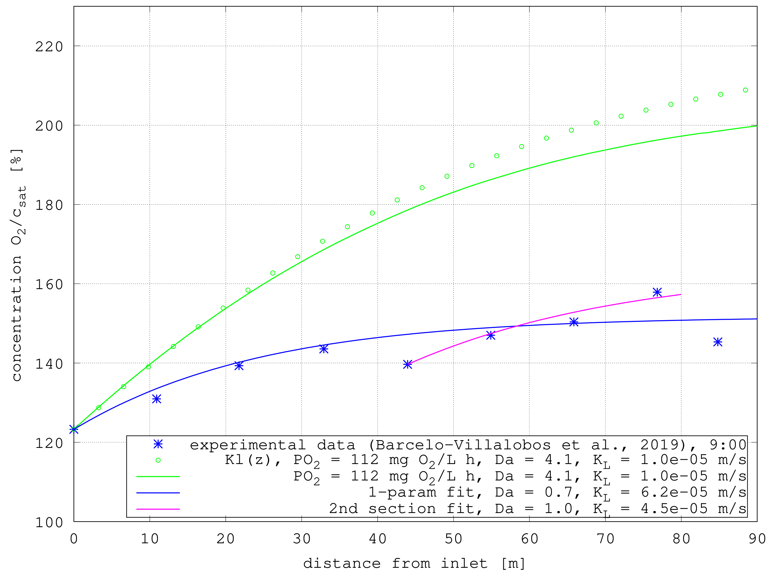
3.3. Comparison with Experimental Data

Experimental data and regression analysis can be used to determine parameters in Equation (7) representing the simplified description of the whole system. Using the measured concentrations along the reactor length as presented by [11], we can find the value of mass transfer coefficient K L (or K L a ) which would fit the experimental data best. The following Figure 5 shows the result for the data set corresponding to the measuring time 9:00 with I av = 129 μ E / m 2 s , which yields PO 2 = 112 mg O 2 / L h according to Equation (1). The fitted value of the overall mass transfer coefficient is K L = 6.2 × 10 5 m s 1 (with 14.5% confidence interval) for all data points excluding the last one, which is much larger than the value used in CFD simulations K L = 1.02 × 10 5 m s 1 (which was based on a separate simulation describing mass transfer in a moving liquid film of constant height and it is illustrated in the figure as well—see the top-most green curve there).
However, concerning the experimental data, there is a visible drop in the concentration between 40 and 50 m distance, which corresponds to the transition between two 40 m long sections of the whole system [11]. Applying the fitting procedure to the data points in the second section only (excluding the last point which was probably in the sump already), the appropriate value of the mass transfer coefficient would be K L = 4.5 × 10 5 m s 1 (with 17.5% confidence interval), which is smaller than the fitted value for the whole system. This is in accordance with the fact that at the beginning of the system, the mass transfer coefficient is larger due to entrance effects. The dependency of mass transfer coefficient on the distance was already illustrated on Figure 2 and described by Equation (5). As it was based on CFD simulation for a 10 m long system only, it would not make sense to apply it to the much longer 80 m system [11]; nevertheless, the top-most green points in Figure 5 illustrates the impact of this dependency on the concentration profile of the dissolved oxygen. It clearly shows that the decreasing value of the mass transfer coefficients along the system length yields in larger concentrations of the dissolved oxygen in the liquid phase. Of course, with longer system the dependency on distance would be different, fitting the experimental data depicted in Figure 5 gives the following correlation:
k l = 8.2 × 10 5 z 0.09 , Sh z = 0.079 Re z 0.91 Sc 1 / 3 .
Here, the exponent of z coordinate is much smaller (−0.09) compared to the shorter system (−1/3), that is, the entrance effects have a much smaller impact. A statistical F-test [25] comparing two variants of the model function fitting the data, one with the power dependency on coordinate z as in Equation (11) and the second one being a simpler model representing a constant value, was performed, and it showed that there is no statistically significant difference between these two models therefore the constant value representing an average over the whole length of the system ( 6.2 × 10 5 m / s , ± 14.5 % ) can be safely used here.

4. Conclusions

In this work, the dissolved oxygen concentration within a thin-layer cascade reactor for microalgae cultivation was simulated using commercial ANSYS Fluent software with user-defined function (UDF) implemented. While the mass transfer phenomena represent a standard problem (embedded within the software package), the reaction term including the inhibition of photosynthetic efficiency by the dissolved oxygen has to be specially modeled. We have also proposed a simplified model based on the ordinary differential equation describing the oxygen profile along TLC system and verified that the results are in good agreement with CFD simulations. Based on the experimental data measured on the TLC reactor located at the IFAPA Research Centre (Almería, Spain), we determined the mass transfer coefficient on the liquid side and illustrated its effect on the photosynthetic oxygen production and consequently dissolved oxygen profiles along the length of the system. The value of the mass transfer coefficient fitted to experimental data was approximately 6 times larger than the value determined in a separate CFD simulation. We see the main reasons of this discrepancy in local variations of the mass transfer parameters which might be difficult to capture without knowing the exact geometrical parameters and performing full 3D CFD simulations.
We underline that the main achievement of this study dwells in the presented methodology, which provides a viable approach of describing microalgae culture systems and gives us a useful tool for the MCS design and possible identification and/or parameter optimization. In the case of TLC-like systems, the proposed simplified ODE model could be used, whereas for more complex geometries and flow patterns, full 3D simulations must be used.

Author Contributions

Conceptualization, Š.P., K.P., and C.I.G.; methodology, K.P. and Š.P.; software, K.P. and C.I.G.; formal analysis, Š.P. and K.P.; resources, Š.P., K.P., and C.I.G.; writing—original draft preparation, Š.P. and K.P.; writing—review and editing, Š.P., K.P., F.G.A.F., and J.M.F.-S.; visualization, K.P. and Š.P.; supervision, Š.P.; funding acquisition, Š.P. and F.G.A.F. All authors have read and agreed to the published version of the manuscript.

Funding

This research was financially supported by the Czech Science Foundation through the research grant No. 19-05872S. K. Petera funding: OP RDE grant CZ.02.1.01/0.0/0.0/16_019/0000753 “Research center for low-carbon energy technologies”. C.I.G., F.G.A.F., and J.M.F-S. funding: This work forms part of the SABANA Project of the European Unions’ Horizon 2020—Research and Innovation Framework Programme (Grant Agreement 727,874), the AL4BIO Project and PURASOL, funded by the Spanish Ministry of Science, Innovation and Universities. C.I.G. mobility co-financed with the ERASMUS + program of the European Union.

Institutional Review Board Statement

Not applicable.

Informed Consent Statement

Not applicable.

Data Availability Statement

Data is contained within the article or cited articles.

Conflicts of Interest

The authors declare no conflict of interest. The funders had no role in the design of the study; in the collection, analyses, or interpretation of data; in the writing of the manuscript; or in the decision to publish the results.

Nomenclature

aspecific surface of interfacial area (m 2 /m 3 )
cmolar concentration (kmol/m 3 )
c L total molar concentration of liquid (kmol/m 3 )
c L , O 2 * Oxygen molar concentration according to Henry’s law, see Equation (4) (kmol/m 3 )
DaDamköhler number, PO 2 / K L c L x O 2 * , see Equation (8) (-)
D O 2 diffusion coefficient of oxygen in water (m 2 /s)
Ilight irradiance ( μ E/m 2 s)
I av average value of I ( μ E/m 2 s)
H O 2 Henry’s coefficient (-)
k g gas-side mass transfer coefficient (ms 1 )
k l liquid-side mass transfer coefficient (ms 1 )
K L overall mass transfer coefficient (ms 1 )
N L molar flux of the liquid phase kmol m 2 s 1
Re z Reynolds number, uz / ν (-)
Sh z Sherwood number, k l z/D O 2 (-)
ScSchmidt number, ν /D O 2 (-)
uvelocity (ms 1 )
x O 2 molar fraction of dissolved oxygen (-)
PO 2 production of oxygen by algae cells (mg O 2 /L h, kmol m 3  s 1 )
PO O 2 , max maximum production of oxygen by algae cells (mg  O 2 /L  h)
zcoordinate, distance from the inlet (m)
ν kinematic viscosity (m 2 s 1 )

References

  1. Chisti, Y. Biodiesel from microalgae. Biotechnol. Adv. 2007, 25, 294–306. [Google Scholar] [CrossRef] [PubMed]
  2. Richmond, A.; Hu, Q. Handbook of Microalgal Culture: Applied Phycology and Biotechnology: Second Edition; John Wiley and Sons: Hoboken, NJ, USA, 2013. [Google Scholar] [CrossRef]
  3. Schädler, T.; Neumann-Cip, A.C.; Wieland, K.; Glöckler, D.; Haisch, C.; Brück, T.; Weuster-Botz, D. High-Density Microalgae Cultivation in Open Thin-Layer Cascade Photobioreactors with Water Recycling. Appl. Sci. 2020, 10, 3883. [Google Scholar] [CrossRef]
  4. Bernard, O.; Mairet, F.; Chachuat, B. Modelling of Microalgae Culture Systems with Applications to Control and Optimization. Adv. Biochem. Eng. Biotechnol. 2016, 153, 59–87. [Google Scholar] [CrossRef] [PubMed]
  5. Ooms, M.; Dinh, C.T.; Sargent, E.; Sinton, D. Photon management for augmented photosynthesis. Nat. Commun. 2016, 7, 12699. [Google Scholar] [CrossRef] [PubMed]
  6. Bernardi, A.; Perin, G.; Sforza, E.; Galvanin, F.; Morosinotto, T.; Bezzo, F. An Identifiable State Model To Describe Light Intensity Influence on Microalgae Growth. Ind. Eng. Chem. Res. 2014, 53, 6738–6749. [Google Scholar] [CrossRef] [PubMed]
  7. Torzillo, G.; Vonshak, A. Environmental Stress Physiology with Reference to Mass Cultures. In Handbook of Microalgal Culture; John Wiley & Sons, Ltd.: Hoboken, NJ, USA, 2013; Chapter 6; pp. 90–113. [Google Scholar] [CrossRef]
  8. Fernández, I.; Acién, F.; Fernández, J.; Guzmán, J.; Magán, J.; Berenguel, M. Dynamic model of microalgal production in tubular photobioreactors. Bioresour. Technol. 2012, 126, 172–181. [Google Scholar] [CrossRef] [PubMed]
  9. Sforza, E.; Pastore, M.; Franke, S.M.; Barbera, E. Modeling the oxygen inhibition in microalgae: An experimental approach based on photorespirometry. New Biotechnol. 2020, 59, 26–32. [Google Scholar] [CrossRef] [PubMed]
  10. Doucha, J.; Lívanský, K. Outdoor open thin-layer microalgal photobioreactor: Potential productivity. J. Appl. Phycol. 2006, 21, 111–117. [Google Scholar] [CrossRef]
  11. Barceló-Villalobos, M.; Serrano, C.G.; Zurano, A.S.; García, L.A.; Maldonado, S.E.; Peña, J.; Fernández, F.A. Variations of culture parameters in a pilot-scale thin-layer reactor and their influence on the performance of Scenedesmus almeriensis culture. Bioresour. Technol. Rep. 2019, 6, 190–197. [Google Scholar] [CrossRef]
  12. Mendoza, J.; Granados, M.; de Godos, I.; Acién, F.; Molina, E.; Heaven, S.; Banks, C. Oxygen transfer and evolution in microalgal culture in open raceways. Bioresour. Technol. 2013, 137, 188–195. [Google Scholar] [CrossRef] [PubMed]
  13. Pawlowski, A.; Mendoza, J.; Guzmán, J.; Berenguel, M.; Acién, F.; Dormido, S. Effective utilization of flue gases in raceway reactor with event-based pH control for microalgae culture. Bioresour. Technol. 2014, 170, 1–9. [Google Scholar] [CrossRef] [PubMed]
  14. Kazbar, A.; Cogne, G.; Urbain, B.; Marec, H.; Le-Gouic, B.; Tallec, J.; Takache, H.; Ismail, A.; Pruvost, J. Effect of dissolved oxygen concentration on microalgal culture in photobioreactors. Algal Res. 2019, 101, 101432. [Google Scholar] [CrossRef] [Green Version]
  15. Sousa, C.; Compadre, A.; Vermuë, M.H.; Wijffels, R.H. Effect of oxygen at low and high light intensities on the growth of Neochloris oleoabundans. Algal Res. 2013, 2, 122–126. [Google Scholar] [CrossRef]
  16. Grivalský, T.; Ranglová, K.; da Câmara Manoel, J.; Lakatos, G.; Lhotský, R.; Masojídek, J. Development of thin-layer cascades for microalgae cultivation: Milestones (review). Folia Microbiol 2019, 64, 603–614. [Google Scholar] [CrossRef] [PubMed]
  17. Grima, E.M.; Camacho, F.G.; Pérez, J.A.S.; Sevilla, J.M.F.; Fernández, F.G.A.; Gómez, A.C. A mathematical model of microalgal growth in light-limited chemostat culture. J. Chem. Technol. Biotechnol. 1994, 61, 167–173. [Google Scholar] [CrossRef]
  18. Costache, T.; Fernández, F.G.A.; Morales, M.; Fernández-Sevilla, J.M.; Stamatin, I.; Molina, E. Comprehensive model of microalgae photosynthesis rate as a function of culture conditions in photobioreactors. Appl. Microbiol. Biotechnol. 2013, 97, 7627–7637. [Google Scholar] [CrossRef] [PubMed]
  19. Ippoliti, D.; Gómez, C.; del Mar Morales-Amaral, M.; Pistocchi, R.; Fernández-Sevilla, J.; Acién, F.G. Modeling of photosynthesis and respiration rate for Isochrysis galbana (T-Iso) and its influence on the production of this strain. Bioresour. Technol. 2016, 203, 71–79. [Google Scholar] [CrossRef] [PubMed]
  20. Bird, R.B.; Stewart, W.E.; Ligthfoot, E.N. (Eds.) Transport Phenomena; John Wiley & Sons, Inc.: Hoboken, NJ, USA, 2002. [Google Scholar]
  21. ANSYS Fluent. ANSYS Fluent Theory Guide; ANSYS, Inc.: Canonsburg, PA, USA, 2021. [Google Scholar]
  22. Chiarini, A.; Quadrio, M. The turbulent flow over the BARC rectangular cylinder: A DNS study. Flow Turbul. Combust. 2021, 1573–1987. [Google Scholar] [CrossRef]
  23. Papacek, S.; Jablonsky, J.; Petera, K. Advanced integration of fluid dynamics and photosynthetic reaction kinetics for microalgae culture systems. BMC Syst. Biol. 2018, 12, 93. [Google Scholar] [CrossRef] [PubMed]
  24. Celik, I.; Ghia, U.; Roache, P.; Freitas, C.; Coleman, H.; Raad, P. Procedure for Estimation and Reporting of Uncertainty Due to Discretization in CFD Applications. J. Fluids Eng. 2008, 130, 078001. [Google Scholar] [CrossRef] [Green Version]
  25. Motulsky, H.J.; Christopulos, A. Fitting Models to Biological Data Using Linear and Nonlinear Regression. A Practical Guide to Curve Fitting; GraphPad Software Inc.: San Diego, CA, USA, 2003. [Google Scholar]
Figure 1. Basic geometry 2-D showing volume fraction of water (red color—volume fraction of liquid is 1, blue color—volume fraction is 0) in the given system. Boundary conditions used in our simulations are depicted in the figure.
Energies 14 07284 g001
Figure 2. Liquid-side mass transfer coefficient k l dependency on the distance from the inlet evaluated in a separate CFD simulation of moving water thin layer of constant height.
Energies 14 07284 g002
Figure 3. Concentration profiles of dissolved oxygen along the thin-layer reactor (along almost horizontal line traced 5 mm from the bottom) and comparison of CFD simulations results with solution of Equation (7). Two variants of maximum value PO 2 , max are depicted here, the basic value 380 mg O 2 / L h , and 5 times larger value approaching the maximum possible concentration representing 225% of the saturated value (depicted as horizontal line at the top of the figure).
Energies 14 07284 g003
Figure 4. Concentration profiles of dissolved oxygen along the thin layer reactor described by Equation (7) for various values of Damköhler number.
Energies 14 07284 g004
Figure 5. Experimental data describing the concentration profiles of dissolved oxygen along the thin-layer reactor [11], and curves based on the solution of Equation (7) with corresponding values of mass transfer coefficient K L . The top-most green data points represent the impact of local dependency of the mass transfer coefficient described by Equation (5).
Energies 14 07284 g005
Publisher’s Note: MDPI stays neutral with regard to jurisdictional claims in published maps and institutional affiliations.

