
Wake Width: Discussion of Several Methods How to Estimate It by Using Measured Experimental Data


1
Faculty of Mechanical Engineering, University of West Bohemia in Pilsen, Univerzitní 22, 306 14 Pilsen, Czech Republic
2
Institute of Thermomechanics, Czech Academy of Sciences, Dolejškova 5, 180 00 Prague, Czech Republic
*
Author to whom correspondence should be addressed.
Energies 2021, 14(15), 4712; https://doi.org/10.3390/en14154712
Submission received: 2 July 2021
/
Revised: 28 July 2021
/
Accepted: 29 July 2021
/
Published: 3 August 2021
(This article belongs to the Section A3: Wind, Wave and Tidal Energy)
Abstract
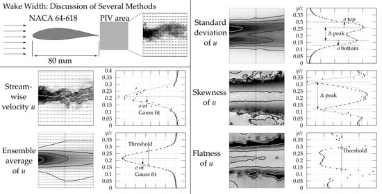
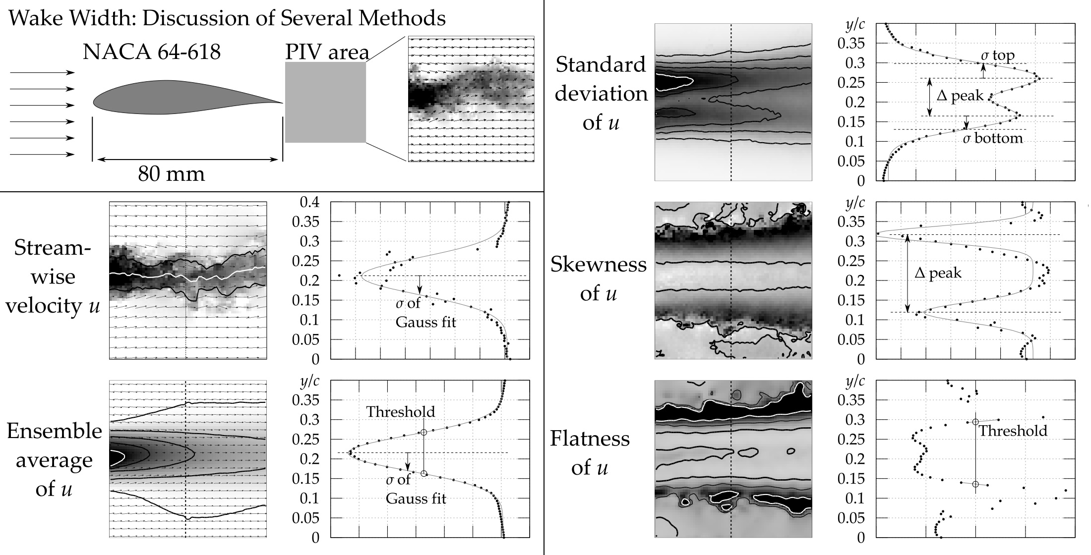
:Several methods of defining and estimating the width of a turbulent wake are presented and tested on the experimental data obtained in the wake past an asymmetric prismatic airfoil NACA 64(3)-618, which is often used as tip profile of the wind turbines. Instantaneous velocities are measured by using the Particle Image Velocimetry (PIV) technique. All suggested methods of wake width estimation are based on the statistics of a stream-wise velocity component. First, the expansion of boundary layer (BL) thickness is tested, showing that both displacement BL thickness and momentum BL thickness do not represent the width of the wake. The equivalent of 99% BL thickness is used in the literature, but with different threshold value. It is shown that a lower threshold of 50% gives more stable results. The ensemble average velocity profile is fitted by Gauss function and its σ-parameter is used as another definition of wake width. The profiles of stream-wise velocity standard deviation display a two-peak shape; the distance of those peaks serves as wake width for Norberg, while another tested option is to include the widths of such peaks. Skewness (the third statistical moment) of stream-wise velocity displays a pair of sharp peaks in the wake boundary, but their position is heavily affected by the statistical quality of the data. Flatness (the fourth statistical moment) of the stream-wise velocity refers to the occurrence of rare events, and therefore the distance, where turbulent events ejected from the wake become rare and can be considered as another definition of wake width. The repeatability of the mentioned methods and their sensitivity to Reynolds’ number and model quality are discussed as well.
1. Introduction and Motivation
Wake is a very important flow structure and is seen often in nature [1]. Broadly speaking, it is produced in an area of fluid which is slowed or stopped by the presence of an obstacle. The shear layers between the slowed and unaffected areas are turbulized and grow toward both directions: (i) inside the wake, turbulizing its interior and transporting surrounding momentum inside, which later leads to an acceleration of the flow and to a “healing” of velocity deficit; (ii) outside of the wake, which results in growth of the area affected by the obstacle and contributes to its smoothing. Thus, the wake is not generally considered to be a structure with an easily definable rigid boundary.
Knowledge of the size of the area, where the flow is affected by some obstruction, has large importance in many engineering applications, starting from design of wind farms [2,3] up to safety of transportation. For example, here in the Czech Republic, a political discussion is taking place about declaring minimal distance of overtaking on a road: especially in cases where a motorized vehicle is overtaking a bicycle. The risk of physical contact is only one half (and, of course, the more dangerous one); the second important issue is the question of when and where the wake of large and fast-moving motorized vehicles reaches the bicycle, with a possible impact on its stability.
It is natural that larger obstacles have larger wakes; however, it is less intuitive that a faster flow produces a slightly smaller wake. The latter is not a general rule, as it depends on the turbulence regime and surroundings. Although the wake lacks a rigid boundary, the information about its width has to be quantified for comparative analysis of various cases and modifications.
A large amount of studies have been published concerning the wake past circular cylinders [1]. The circular cylinder is an easily accessible prototype of a general bluff body. An essential feature occurring in a large range of Reynolds numbers is the stable configuration of alternating vortices discovered by Theodore von Kármán [4], which are responsible for periodic acoustic oscillations described by Vincenc Strouhal (his given name is sometimes spelled as Vincent or Čeněk. The latter form is the Czech form derived from the Italian form Vincenzo (read “Vinčenc”)), in his famous work [5]. Although a cylinder is a prismatic (2D) shape, the wake turbulence displays three-dimensional characteristics [6,7] in dependent regimes. Several regimes [8,9,10] have been detected in essential cases in those which have a dependence on Reynolds number only, and many more, when the surface roughness, surrounding turbulence or angle of axis were taken into account.
The evolution of the wake is one of the key issues in aerodynamics, because this phenomenon can characterize the various effects that occur when flow passes an airfoil [11,12,13]. It should be noted that the deficit of velocity is closely related to the drag force, which can be derived solely from the velocity and pressure in a plane in the wake of the object [14].
In the most cases, PIV, hot wire, or pressure systems are used to estimate wake topology. The first two methods allow us to estimate not only the width and depth of the perturbation area, but also to investigate the structure of the turbulence flow. Classically characteristic wake dimensions are determined by the distribution of the average velocity behind airfoils [15,16]. However, in some cases, they are estimated using the Reynolds stress components and degree of anisotropy of the flow. A comparative assessment of these analyses allows us to clearly define the boundaries of the wake and to determine the transit zone around it [17]. This analysis is especially useful in the study of asymmetric profiles, because in this case, the flow structure around the wake is more complex.
The present paper focuses instead on the wake following an asymmetric airfoil NACA 64-618, which belongs to the family of “streamlined bodies”, although, as will be shown, the real manufacturing procedures do not allow it to reach this idealized state. We focus on a single question: how thick (or wide) is the wake? We offer few definitions, all based on statistics of stream-wise velocity, because this velocity component is easiest to measure by using multiple measuring methods such as Particle Image Velocimetry, Hot Wire Anemometry or Fast Response Aerodynamic Probe.
2. Materials and Methods
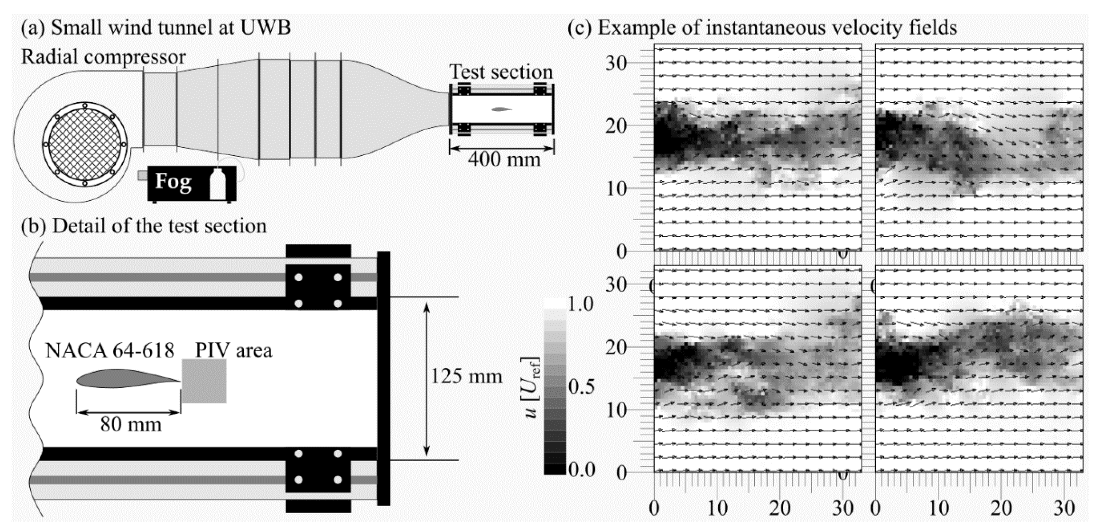
In this contribution, a few methods for evaluation of wake width are compared. For this purpose, sample data are used; these are obtained by using commercial Particle Image Velocimetry [18,19] system in an area past the asymmetric prismatic airfoil NACA 64(3)-618. The “slow” PIV is provided by Dantec Company, which consists of 4 MPix camera FlowSense Mk II and solid-state double-pulse laser New Wave Solo of 500 mJ in single shot; the maximum repeating frequency of the system is 7.4 Hz. The field of view (FoV) is divided into a grid of 64 × 64 interrogation areas, each covering an area of 532 × 532 μm. The velocity vector detection is performed by using the Dantec Dynamic Studio software. The studied airfoil has been printed by using 3D printer Prusa Mk 2.5 and it was made of Polymerized Lactic Acid PLA [20]. More details about the observed flow in the wake at different Reynolds numbers and two angles of attack can be found in our publication [21]. For comparison, the data at chord-based Reynolds number Re = 3.1·104 are selected, and the angle of attack is α = 0°. It should be noted that current experimental setup is not ideal, due to the relatively high blockage ratio—the airfoil chord is equal to 80 mm and the maximum thickness of 14.5 mm, this is inserted into test section of width 125 mm (see the sketch in Figure 1).
3. Discussion of Wake Widths
3.1. Expanding Boundary Layer Approach
In contrast to wake studies, the set of boundary layer (BL) studies has unified standards for estimating the BL thickness. Again, BL is not a structure with some rigid boundary, the thickness is only an imaginary value, but its precise definition allows exact comparison and scientific exploration of questions regarding the effect of surface quality, surrounding turbulence intensity, pressure profile, etc. The main BL thicknesses is comprised of the 99% boundary layer thickness , i.e., the distance, where the average velocity serves as the function of distance from the solid wall y until it reaches 99% of the surrounding velocity ,which we discuss herein. The displacement thickness , is additionally based on the average velocity profile:
The integration goes from the solid surface (0) to infinity or, practically, “far enough”. Its physical interpretation is that it is the shift of an average streamline due to the presence of the solid surface [22,23].
The second main BL thickness definition is the momentum thickness
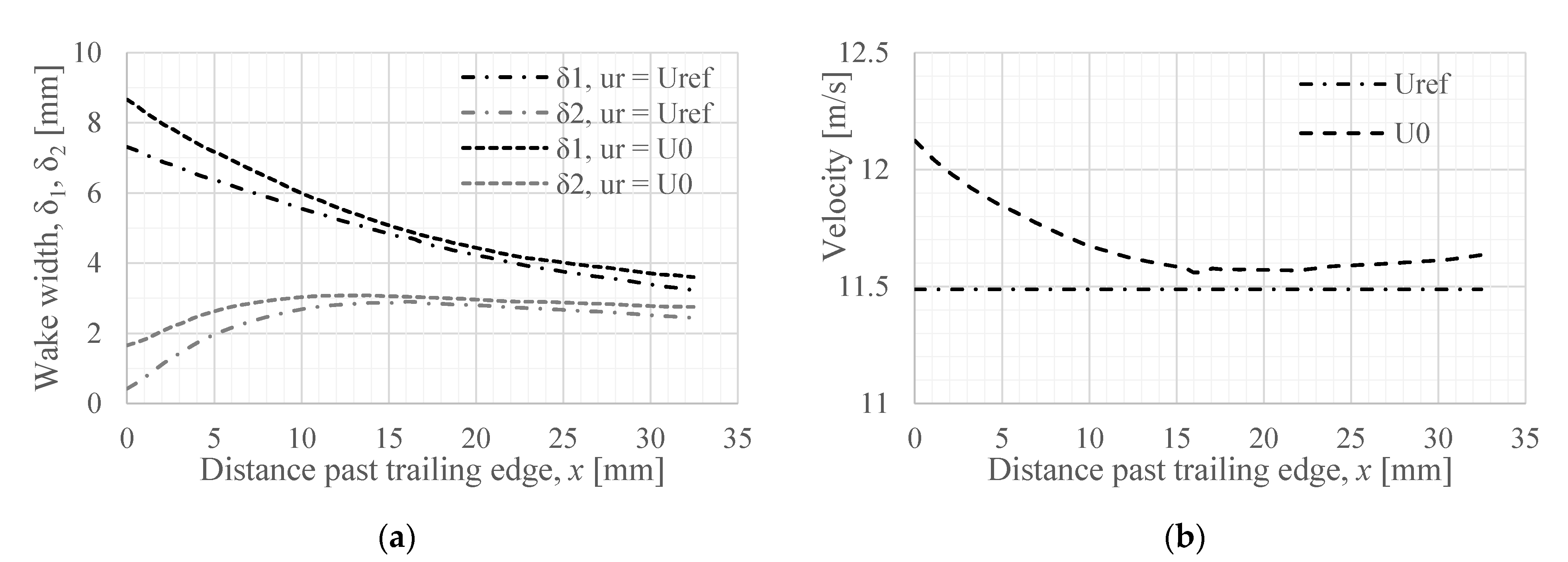
Its physical interpretation is that is the height of hypothetic area, whose momentum is missing from the flow if the velocity profile was unaffected. The main ambiguity of these two definitions is the choice of . At first look, it is clear. However, in the wind tunnel experiments with incompressible fluid, for example, the surrounding velocity is accelerated due to the presence of growing BL. Thus, one may ask which is better: the actual in each position x, or an artificial constant independent on x? This question is much more actual in the case of wake past an obstacle—see the last isotach in Figure 2a, which demonstrates area with ensemble average velocity larger than the ongoing velocity , which is the first natural choice for . However, the actual surrounding velocity may change with the distance (see Figure 3b). This is not only the issue of wind tunnel measurements; the in-field data can easily contain some velocity gradient as well. Figure 3a shows that the choice of this parameter can influence the result significantly.
The main “problem” with expanding the BL approach into the wake is that the measured wake width in fact decreases with stream-wise distance. This is caused by the healing effect of the wake, when the centerline velocity deficit vanishes, and thus the streamline of average velocity field returns toward its unaffected trajectory. The momentum thickness refers to the forces and drag coefficient, rather than to the width of the wake. However, there has been a great deal written about the relation of velocity profiles to the drag coefficient, e.g., [14,24,25,26] and many others.
To conclude, and surely offer an interesting measure of the wake, but their interpretation of wake width is misleading, because they do not describe the widening of the wake.
3.2. Threshold of Average Velocity
The natural and straightforward method is to look where the velocity reaches threshold θ:
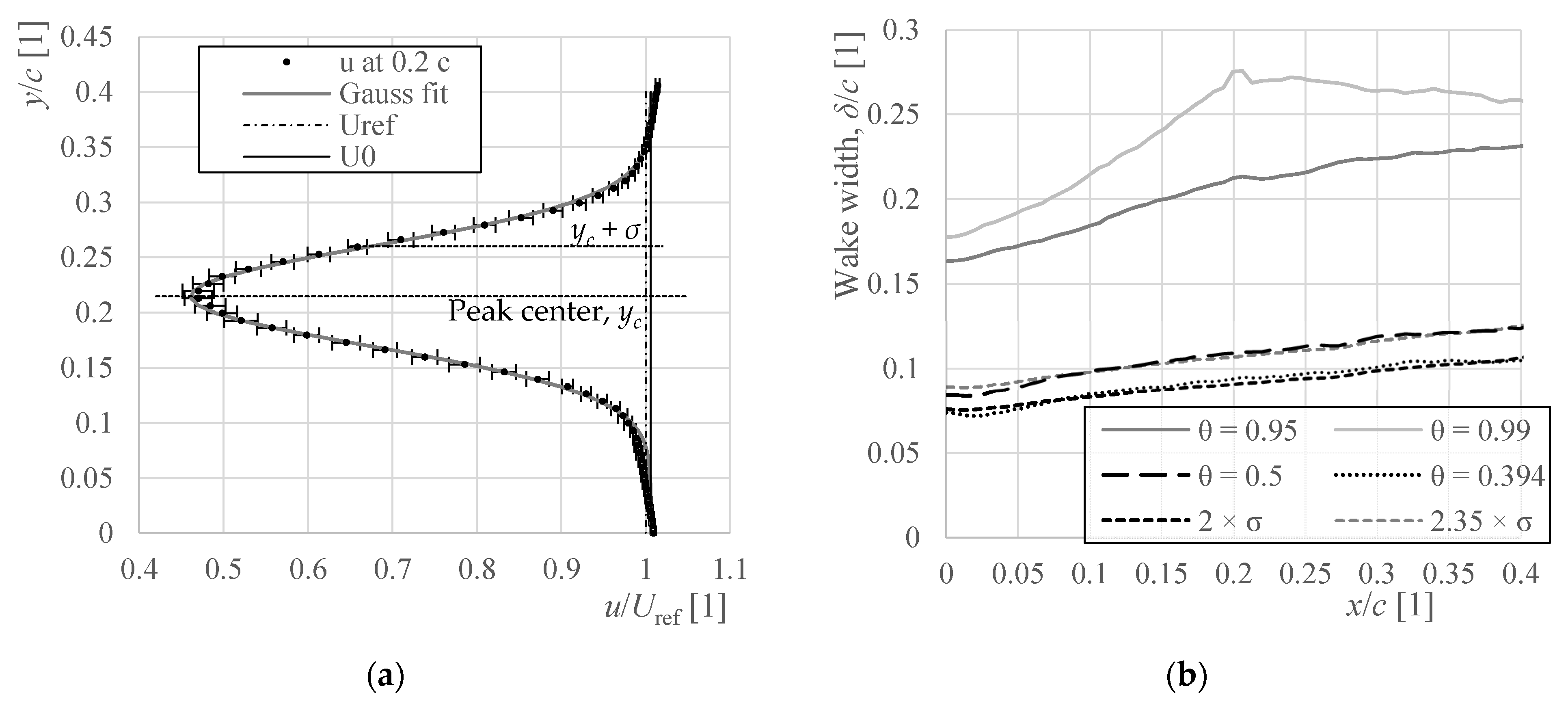
where is the minimal velocity across the wake at a fixed stream-wise distance of x. This approach, where is used by Barthelmie and coworkers in their study of wakes past offshore wind turbines [27]. It is similar to the “99% BL thickness”, with the difference that the threshold is related to the maximum velocity deficit, not to the absolute value of velocity. Here, the problem with the artificially chosen value of repeats as discussed above. An additional artificial parameter is the value of threshold θ—why should one value be better than another? Figure 4a shows that the choice of 99% is not ideal, as it is too close to the ambient flow, and thus the results depend on variations of ambient velocity and uncertainties of measurement. One such issue is observable in Figure 4a as the bump in the middle of field of view, which correlates with a similar bump in the spatial distribution of velocity (Figure 2a) and with drop of the fitted background velocity in Figure 3b; the reason being the connection of two camera chips at that location. However, any study of flow geometry should be independent on such a small instrumental bug. The Barthelmie’s choice of 95% is more robust, but then one may ask, why not 90% or 85%? Here, we try to set this threshold to 50%. The threshold of ½ is advantageous, as the average velocity gradient is steep around that position and therefore the result is less dependent on the small perturbations in surrounding velocity and on the measurement uncertainty—in Figure 4a, the corresponding line is smoother. A last displayed option is , which is the drop of Gaussian function at distance of one σ from its center, , which is the “distance” from background, where the distance from minimum is .
3.3. Gaussian Fit of Average Velocity Profile
In fact, the threshold-based width wake depends only on few measuring points—the local minimum and then a pair of point of each side of the wake to determine the threshold position. Therefore, it is sensitive to random rough measuring error at one point. The fitting procedure uses all measured points, and thus single noisy point cannot destroy the result. Conversely, fitting needs a priori knowledge of the velocity profile shape. The Gauss function occurs in many cases in nature as a product of the Central limit theorem, which is valid for random processes. However, turbulence is not a random process, despite appearing random at first glance [28].
Blondel et al. [29] use super-Gaussian with a power slightly different from 2 to fit the velocity profile past a wind turbine rotor. This leads to better convergence, especially closer to the obstacle. However, too close to the obstacle, this does not work, because the wake contains too strong a “fingerprint” of the obstacle geometry. In Blondel’s case [29], there is a sharper peak past the wind turbine hub surrounded by top-hut wake that is caused by the partly transparent wind turbine rotor. In our case, the velocity gradient is steeper past the pressure side (bottom in figures) than past the suction side—see Figure 2b, where the profile denoted “0” is evidently skewed towards the pressure (bottom) side.
The location of point, where the ensemble average stream-wise velocity reaches one σ of the Gauss function, lies approximately inside the wake, therefore it may be multiplied by a certain constant in order to shift it systematically towards the real wake boundary. When one wants to mimic the value, where the velocity drop reaches half of the centerline drop, then σ must be multiplied by to get the distance of those points multiplied twice, the multiplicator is 2.3548. In this way, any desired level (e.g., 95% or 99%) can be reached without being affected by uncertainty in the surrounding velocity or noise in the velocity profile. Still, as this is just multiplication by constant, this step can be skipped for comparative studies, as done by I. Eames, C. Jonsson and P.B. Johnson [30] in their study of growth of wake past circular cylinder.
3.4. Statistics of Instantaneous Wakes
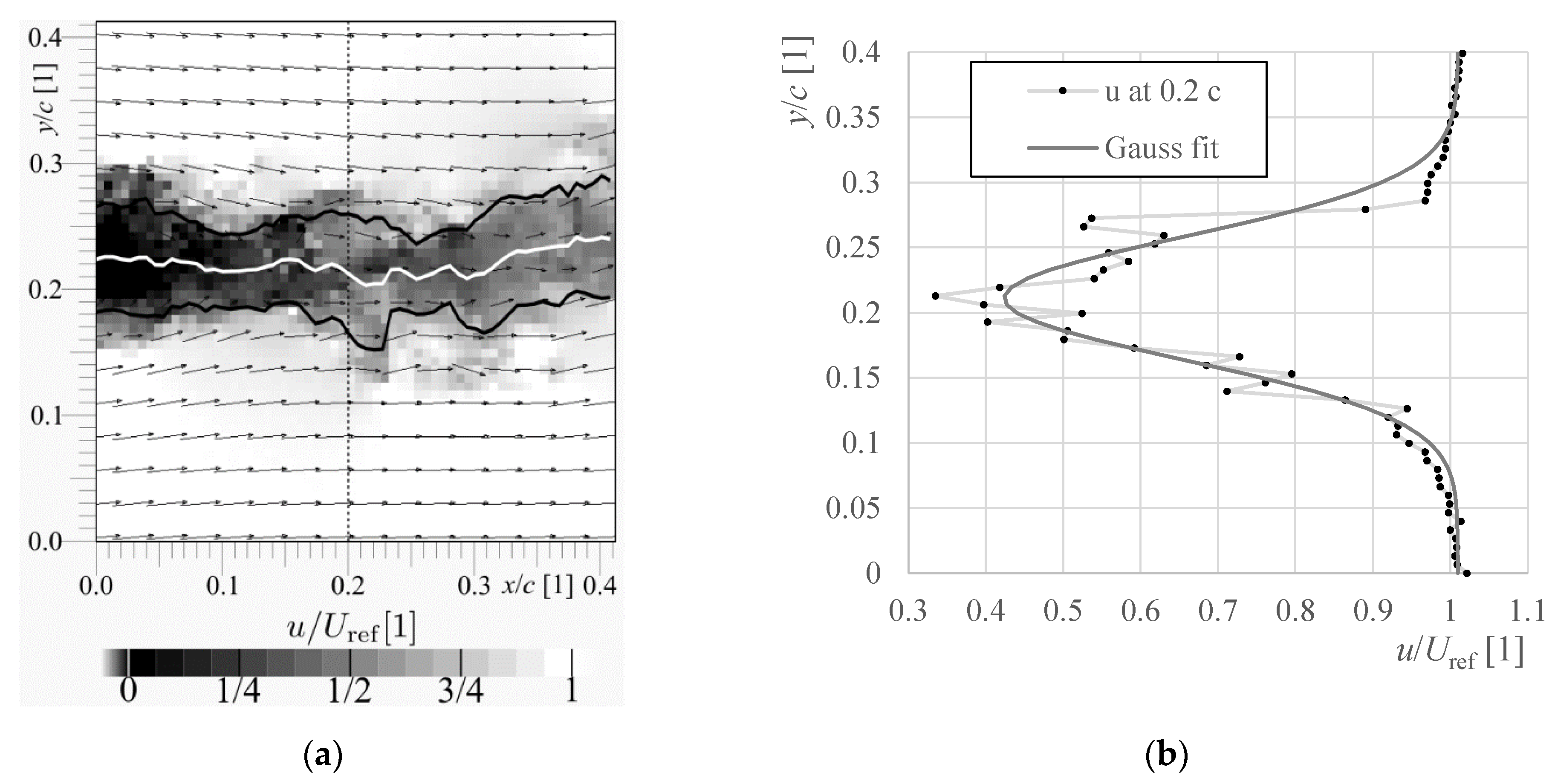
All the other described methods are based on averaged wake structure. However, that average wake is far different from the instantaneous picture, which shows not only widening of the wake, but its meandering as well. Detection of the wake on instantaneous snapshots is possible by fitting the transverse profile of the instantaneous stream-wise velocity by using the Gaussian function. These converge less than that of the average velocity profile because the profile shape deviates from the curve erratically (see Figure 5b), however, the wake centerline and width can still be extracted. Figure 5a shows the found position of wake center and wake width on a single snapshot.
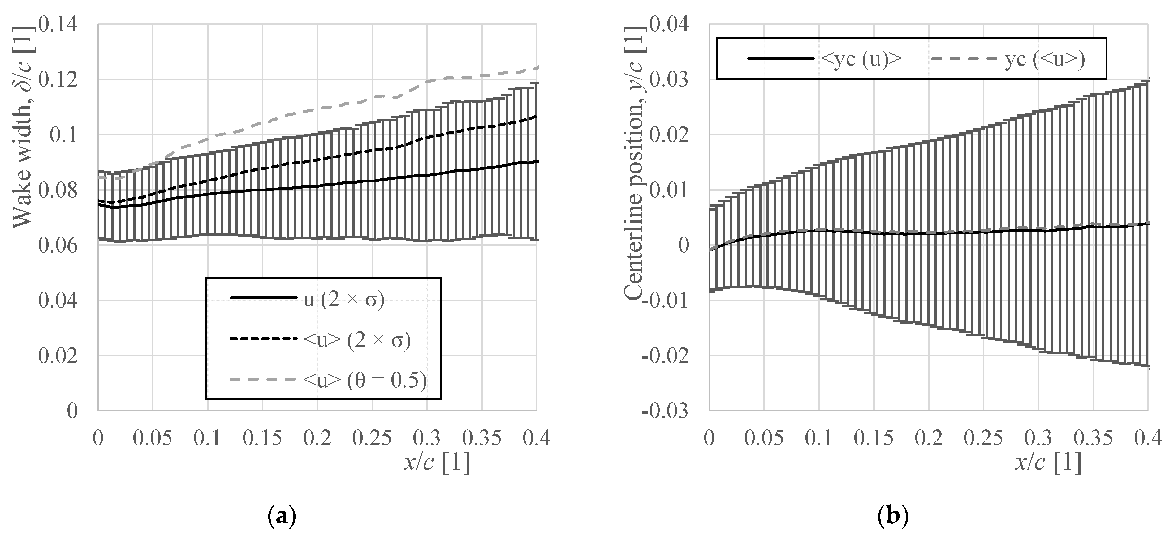
The ensemble average and standard deviation of the found wake widths for each stream-wise position past the trailing edge are displayed in Figure 6a. Close past the trailing edge, the average of instantaneous wake widths corresponds to the width of average wake, while it shows larger discrepancy in later stages. This issue reveals an important fact, that the actual wake is smaller than visible in the averaged data, because part of its width is caused by the meandering of its position. The meandering of the wake affects the standard deviation of the wake center position, which is displayed in Figure 6b in terms of error bars. The difference between the average of instantaneous wake widths and width of the average wake at end of the field of view, x/c = 0.4, is 0.017·c, while the standard deviation of the wake position at same location is 0.026·c.
3.5. Standard Deviation of Stream-Wise Velocity
An important aspect of turbulent wake is the increase of turbulence inside it. The turbulence can be easily quantified by using the standard deviations of the measured velocity components:
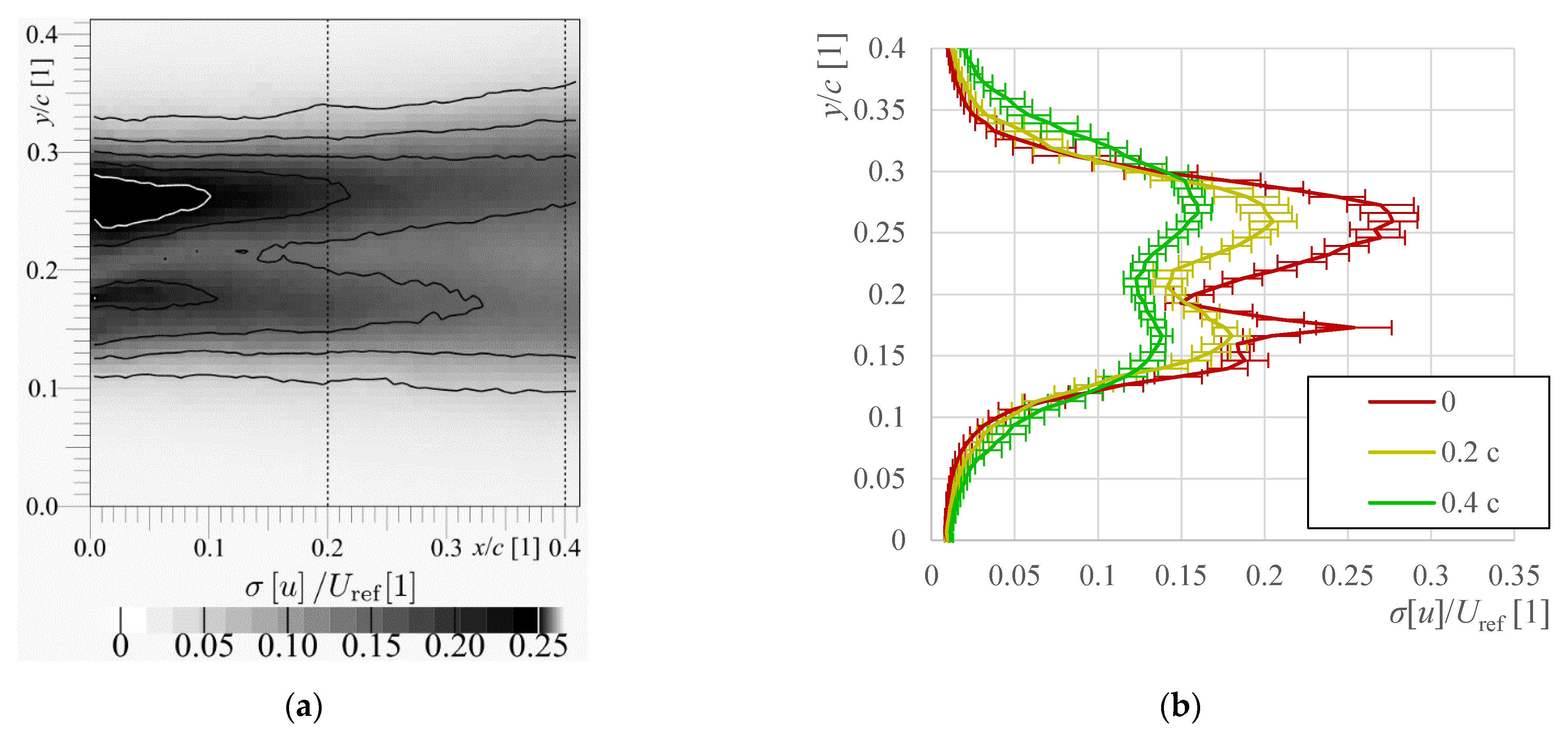
In the wake past a streamed body (which is the case of airfoils under non-stall conditions), the fluctuation wake pattern is dominated by double maxima of the stream-wise component, which form past the boundary layers. In the case of the asymmetric body, these maxima are asymmetric, as can be seen in Figure 7. Here, the bottom maximum past pressure side is smaller than the top one past the suction side, due to the development of boundary layer under different pressure gradients. Near the wake axis, the fluctuations moving in a transverse direction dominate, which is caused by the separation at the trailing edge and the alternating dominance of one or the other boundary layer. In the wake past a bluff body, this effect would be dominating over the entire wake. A second reason why we want to explore the standard deviation of stream-wise direction, rather than Turbulent kinetic energy or the standard deviation of transverse velocity component, is that this velocity component is easily obtainable by other methods e.g., by single-wire Hot Wire Anemometry (HWA) or by fast response pressure probes (FRAP).
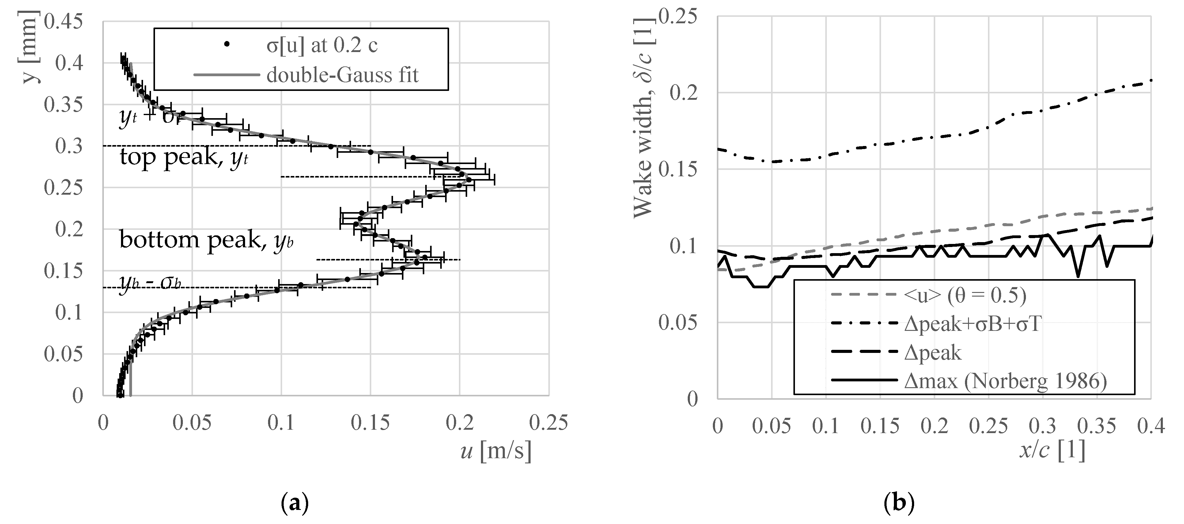
Norberg [31] investigated the flow around the circular cylinder. Among others, he looked for the point of minimal wake width, because, at that position, the vortices are fully formed and start their diffusive convection downstream (he states). As a side product, he suggests the definition of wake width as the distance of maxima of stream-wise velocity fluctuations. This definition is used in [32], and the application of this approach to our data is displayed in Figure 8b as a solid line. A strong “leveling” is caused by the finite resolution of our PIV grid. To avoid discretization of the maxima positions, the fitting procedure can be used again, now with the double-Gauss function:
where B is the background, At and AB are the amplitudes of top and bottom peak respectively, yt and yb are the peak positions and σt and σb are the corresponding peak thicknesses. Again, an a priori expectation of the profile functional dependence is needed, whose validity is limited—see the poor convergence at the bottom part of the profile in Figure 8a. Conversely, the high number of fitting parameters are able to fit almost universally, and thus the physical interpretation of convergence can be easily misleading. The distance of double-Gauss peaks is displayed as a dashed line in Figure 8b. This value is systematically larger than Norberg’s approach, but the development with distance is clearly smoother as all profile points are used instead of single maximum only, which can be easily shifted by local noise.
The distance of peaks does not contain the splashing of the fluctuation structures. In order to adhere to it, we combine this distance of double-Gauss peaks plus widths of peaks. In respect to the average velocity profiles, the latter method is able to distinguish the reduction of wake width in the near wake (at around x/c = 0.05 in Figure 8b), because the double-Gauss function is more robust to the non-ideal shapes of profiles caused by the “fingerprint” of obstacle geometry.
The first and second statistical moments displayed hitherto show a smooth vanishing with increasing distance from the wake axis. Therefore, the wake width cannot point to some exact boundary of the wake, it can only show where it is weak enough. Any one of these methods (when used systematically) can tell us how wake width develops with distance or with Reynolds’ number, or if some shape modifications increase or decrease wake width; and it is capable to answer many more interesting questions. However, is it possible to point to some distance and discern: “the wake ends here“? If our results are confirmed then we feel the answer to this is yes.
3.6. Flatness—The Fourth Statistical Moment
The fourth statistical moment is called Flatness, sometimes (e.g., in Wikipedia) Kurtosis, and is defined as:
It is normalized by standard deviation σ[u], and therefore is dimensionless. It is possible to prove that F[x] of some Gaussian-distributed random quantity x is equal to 3, which is then a reference value.
The physical interpretation of this statistical quantity is that it refers to strong rare events (in popular statistics, they are called “black swan”); in turbulence, they refer to intermittency [28], which shows that turbulence is not a set of random events, but a set of coherent structures—vortices. This is much stronger in quantum turbulence [33], where the vortices are quantized, all having the same circulation; they do not overlap, and therefore if the turbulence intensity is weak, there are merely fewer vortices instead of weaker vortices in classical turbulence. The consequence is that the velocity probability distribution deflects from Gaussian distribution to a polynomial distribution [34] with exponent −3, whose flatness converges to infinity instead of 3 as it does for Gaussian distribution [35]. But at larger scales, the quantum turbulence mimics the classical one, including the higher-order effects such as steady streaming [36].
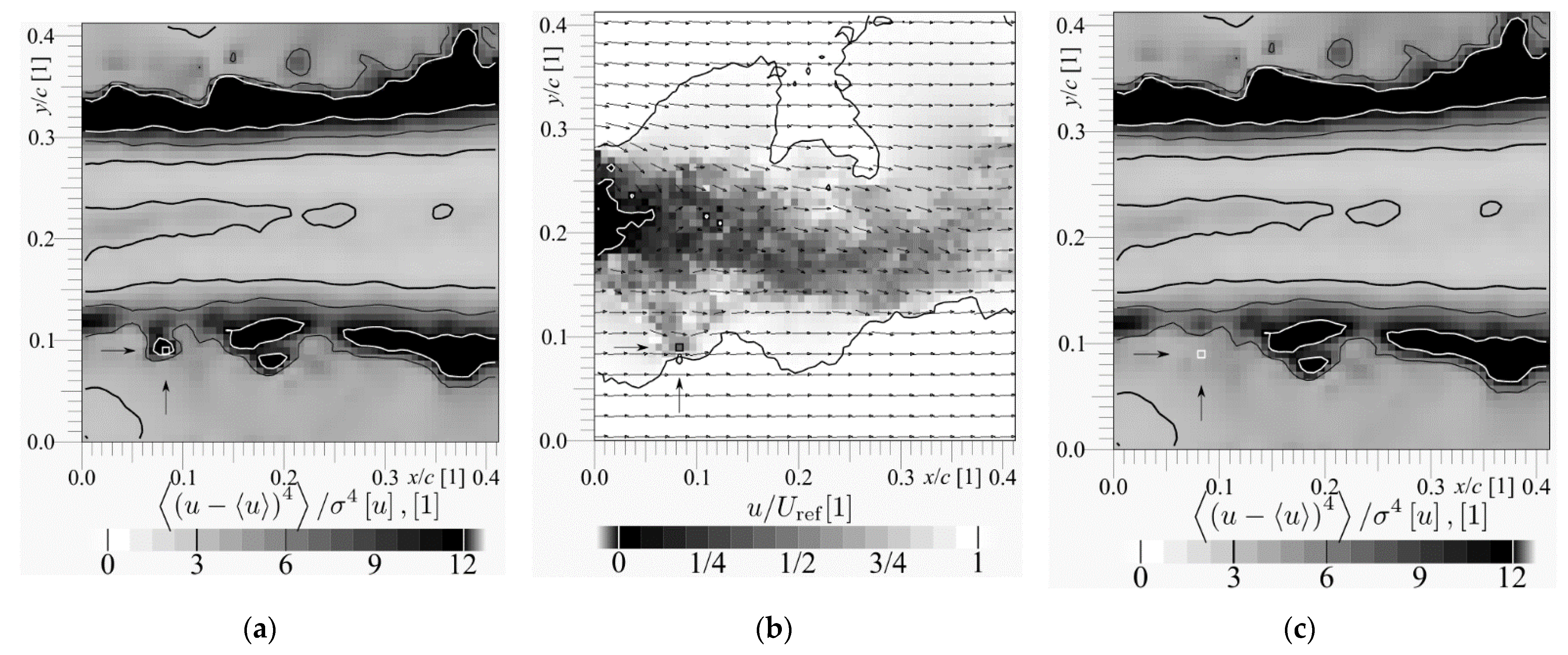
In the case of wake turbulence, the high flatness signal tells us, that there is flow with some turbulence intensity, which is, time-to-time, visited by some structure stronger than would correspond to the usual statistical distribution, which will be demonstrated in a single case. Figure 9a shows the spatial map of flatness of the stream-wise velocity component; note, for example, the local peak in the left bottom corner denoted by white rectangle and black arrows. Figure 9b shows the snapshot, which differs most from the ensemble average at the denoted point. It is a regular snapshot with no more noise than the others, only here is some turbulent structure, which ejects the low-momentum fluid from the wake into the faster surroundings. This is not against the rules, but it is a rare event. This event produces high flatness signal, which is proven in Figure 9c, showing the flatness of all other snapshots. Consequently, the signal around the denoted point refers to regular fluctuations, thus flatness is slightly larger than 3.
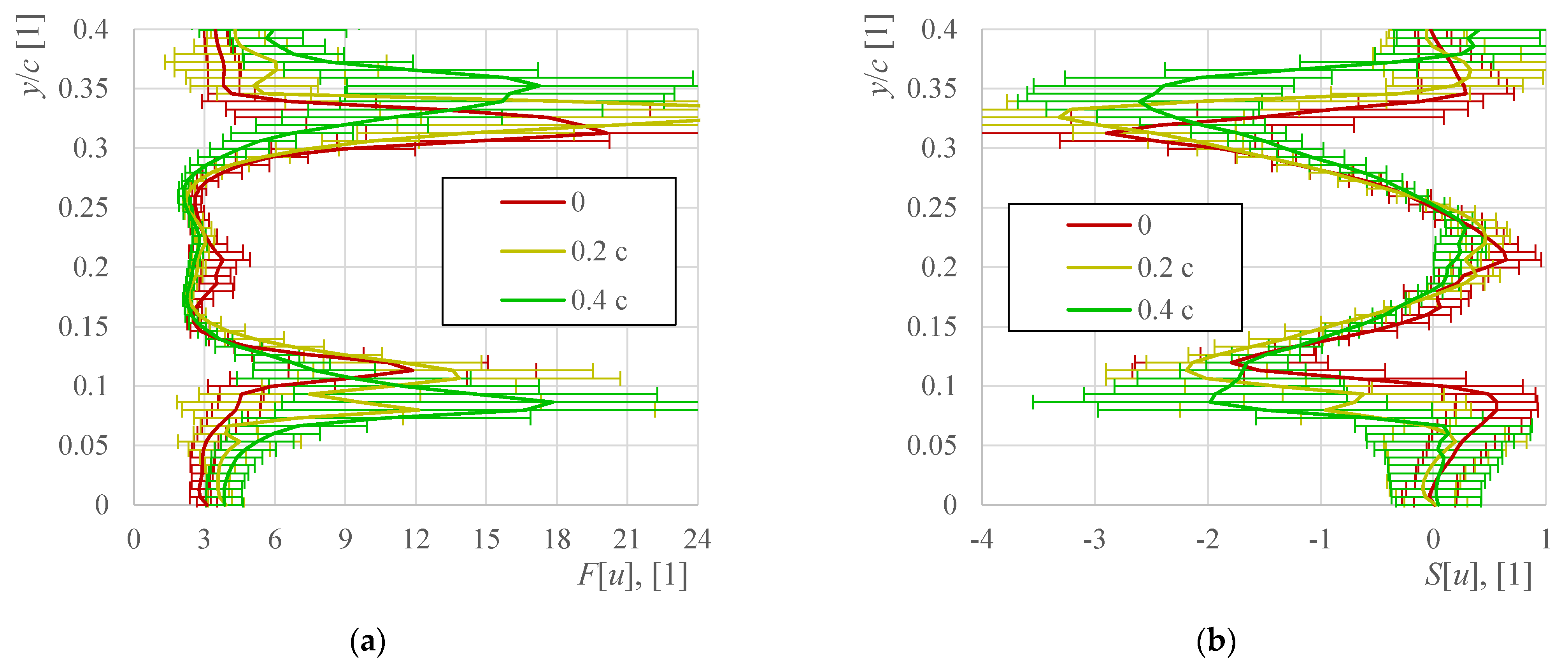
This behavior of flatness inspired us to define the wake boundary as the line, over which the fluctuations become rare, i.e., where flatness grows over 6 (twice the Gauss reference value). The growth of flatness is quite steep, and it grows to large values, see Figure 10a. The main disadvantage is that it needs high statistical quality of the ensemble: there are over 1200 snapshots, which is not a small amount, and the flatness map is still irregular, especially at the outer boundary. Just one snapshot with wrong data can easily disturb flatness value. The uncertainty of flatness is especially high in the case of PIV data (see error bars in Figure 10a), however, the flatness increase is steep enough to give a reasonable wake boundary localization despite the large uncertainty.
The average velocity itself could lead easily to misleading conclusions. For example, imagine an observer staying somewhere next to the wake. When taking into account the average velocity and turbulence intensity only, one would expect that the observer observes velocity slightly smaller than the surrounding one, with turbulence intensity slightly larger. However, they in fact observe the surrounding velocity and turbulence intensity most of the time, with only few blows of the wake fluid. This is an important difference, especially for the problems of mechanical stability or turbulent mixing.
3.7. Skewness—The Third Statistical Moment
The asymmetry in velocity distribution can be quantified in terms of the skewness, sometimes called coefficient of asymmetry, defined as the third central statistical moment:
At the boundary of the turbulent wake, the average velocity is smaller than in the surroundings, which is caused by the mixing with wake fluid. When the shear layer is visited by the slower fluid from the central region, then this visit likely decreases the velocity here more than it increases it. This asymmetry produces negative skewness signal at the wake boundary. Conversely, in the central region, the visit from outside increases the velocity, thus the skewness is slightly positive there.
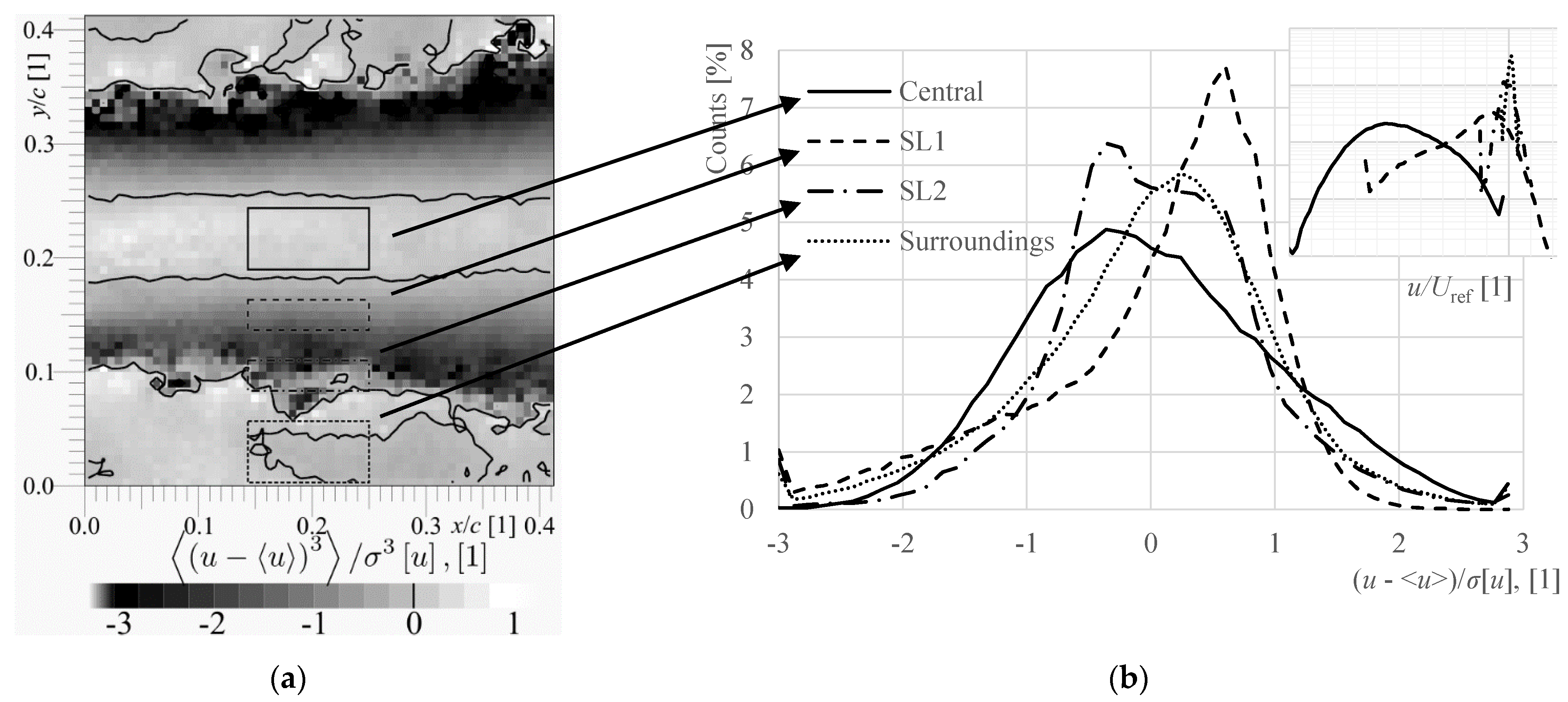
Figure 11a shows the spatial distribution of stream-wise velocity skewness across the field of view with four depicted regions. Figure 9b displays the probability density of instantaneous variations of u in those regions. The central region is almost symmetric, however, note that the maximum occurrence (peak in the solid line in Figure 11b) has shifted in respect to the average (zero in the horizontal axis in the plot). The inner part of the shear layer (dashed line denoted SL1) displays a higher amount of slower events than faster events; the outer shear layer region (SL2, dash-dotted line) contains two merged peaks, and the surrounding region displays distribution more like the Gaussian. Note that it is much sharper in absolute values, see the inset of Figure 11b.
It has been reported by A. Mariotti and G. Buresti [37], that skewness of stream-wise velocity past a bullet-like body (the head is a rotating ellipsoid of 3:1 axis ratio; the body is a cylinder with a sharp base) contains negative peak in the transverse profile and that the position of this peak corresponds to the downstream projection of the obstacle surface. Their work inspired us to define the wake width as the distance of pair of negative peaks in stream-wise velocity skewness. The skewness transverse profiles past NACA 64-618 airfoil are displayed in Figure 10b. Note that the wake past a bluff body may not contain such sharp peaks; the pattern of skewness is similar to that of flatness. It is not a random coincidence—both statistical moments reflect the same phenomenon of mixing the fluids from wake center and from surroundings.
Figure 12 shows the wake width determined via double-Gauss fitting of skewness (triangles) and via thresholding of flatness (squares). The (ir)regularity of their development reveals that the usage of all profile points during fitting procedure does not need to be advantageous in all cases: the poorer statistical convergence at the outer wake boundary is inherited within the position of skewness peaks, while the threshold at inner part of the wake boundary is more stable. Unfortunately, some meaningful threshold value for the skewness profile is unknown at this moment. In the case of Hot Wire Anemometry (HWA) or Laser Doppler Anemometry (LDA) the statistical quality is not a problem, because those methods are capable to gain millions of data points at each location, while PIV method used here is limited to the maximum thousands of snapshots.
4. The Effect of Reynolds Number
Exploring the wake widths at different Reynolds numbers (Figure 13) reveals one important detail: the described methods based on higher statistical moments may not work under laminar conditions. It is not surprise, because the laminar flow does not contain fluctuations. The only source of fluctuation is the random time of snapshots (the acquisition system not synchronized with the vortex shedding in laminar wake). The average of instantaneous wake width shows the same values as the Gaussian-fitted value on average velocity field in the laminar regime at Reynolds numbers 1.6 and 2.0·104, while the meandering of the centerline expressed as the standard deviation of its ensemble-averaged positions reaches maximal values at lowest Re (see Figure 14b, circles). The laminar wake is a different pattern than the turbulent wake, therefore different methods shall be applied for its exploration.
Figure 14 shows the wake width determined by discussed methods at fixed position past the obstacle, but this plot does not contain the information about the wake development with distance past the obstacle. Eames et al. [30] derived that the functional dependence of wake width follows the square root of the distance past obstacle, because as the turbulence intensity decreases due to splashing, there is less energy to eject turbulized fluid out. However, this effect takes place in developed wake, while the example used here covers only the near wake region, where the development of wake width with distance roughly follows a simpler linear function (see Figure 12 and Figure 13) since the position x/c = 0.1:
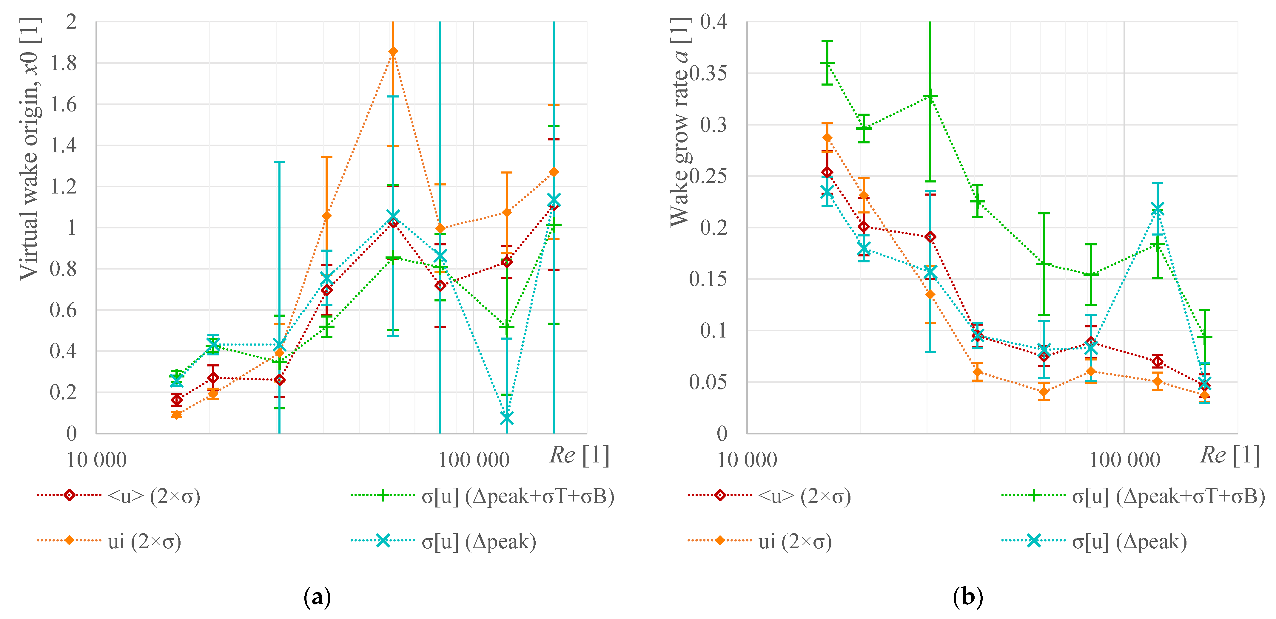
where a is the wake grow rate (Figure 15b) and x0 can be understand as a virtual origin of the wake upstream the obstacle trailing edge (Figure 15a). If we imagine that the wake widths discussed here differ only by a scale, then the parameter a differs as well, but the parameter x0 might reach same values. Figure 15a shows that it is the case at lower Reynolds numbers in a laminar regime, while at higher Re, x0 differs among methods. The methods based on average velocity display origin closer to the trailing edge, while the methods employing fluctuations virtually originate farer upstream. All points display grow with Reynolds number (i.e., originating farer upstream), with an increase in the range of transient flow from laminar to turbulent regimes. The linear wake grow rate systematically decreases with Reynolds number, except for the transient area. Therefore, one can expect that this airfoil produces a smaller total wake area, including the unobserved downstream development at higher Reynolds numbers, which physically supports the observation of Du et al. [38] that this airfoil has a good performance at higher Re. The wake width, which is affected less in the transition regime, seems to be the wake width based on stream-wise fluctuations; this width displays the largest grow a.
5. Uncertainty
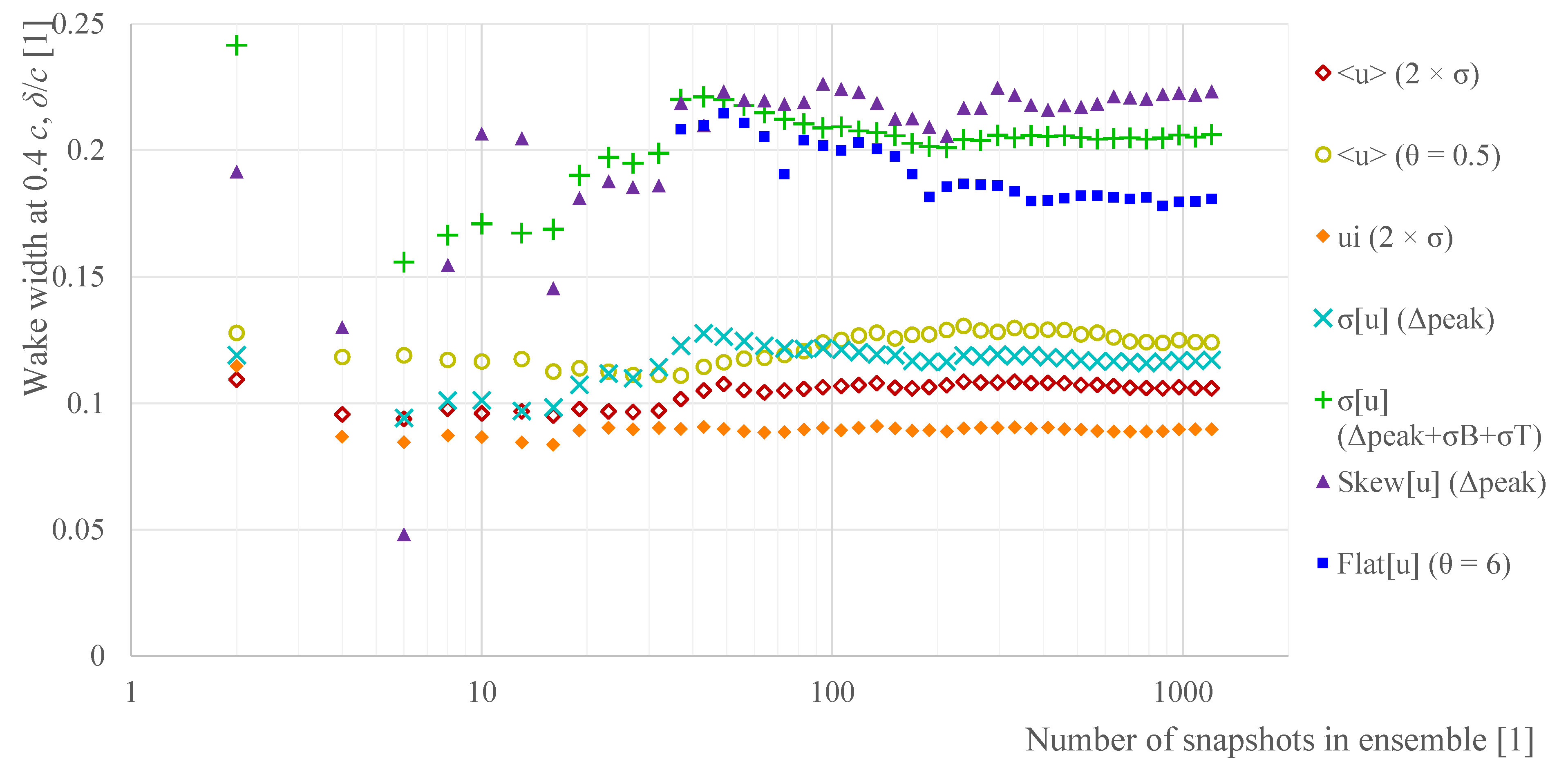
The uncertainty of such a complex method, as PIV is, consists of many error sources [39,40] starting from the image preprocessing, through cross-correlation peak detection up to statistical issues. Generally, the measurement uncertainty projects into two main effects: systematic error and statistical noise. The systematic error in velocity does not affect the wake width, which is a geometrical property, but it is affected by the uncertainty in calibration (which affects the measured velocity as well) and in boundary conditions (input velocity, geometry of the tunnel and obstacle). It is difficult to beat the systematic error without applying some other method, which would have its own sources of uncertainty. Conversely, the statistical noise is naturally present in any measured series and its level might decrease with the number of samples as [40]. Its effect is illustrated in Figure 16, showing the wake widths obtained by several discussed approaches as a function of number of snapshots taken into account. At smaller numbers of snapshots, all methods give untrustworthy results; the fitting methods stabilize after approx. 100 points, the threshold of average velocity definitely needs more, while the methods based on higher moment do not seem to stabilize at all. This empirical approach is used to estimate all the uncertainties presented in this work: the ensemble is virtually separated into 10 subsets; the analysis is performed on each of them, and the standard deviation of the set of results is used as the estimation of unknown uncertainty.
6. Conclusions
The present article compares several methods of calculating wake width. All mentioned methods are based on a transverse profile of the stream-wise velocity component, because this component is accessible by most measuring techniques. Basically, the wake width can be found from points, where the profile of a given quantity reaches a chosen threshold, or as a result of fitting procedure, where some functional profile shape has to be known. The advantages and disadvantages are listed in Table 1. Table 2 compares the statistical momenta of stream-wise velocity components, which can show the wake boundary. As it is often in such cases, the property, which is advantageous for one application, can be disadvantageous for another, and vice versa.
To give some final recommendations, the wake width based on an average velocity profile would be excellent for comparative studies, to determine which variant of some construction element creates smaller wake. When the research goal points to mixing problems, to mechanical stability of other construction elements near the wake, to transportation safety issues or to the interaction of multiple wakes, then the higher statistical momenta must be taken into account, however, the skewness seems to behave too irregularly, and therefore the flatness remains.
Future Work
The present data have been measured past a prismatic airfoil inside a wind tunnel with minimal turbulence intensity. A natural question is how the discussed wake widths would behave in the case of moderate or even high turbulence intensities, especially the skewness and flatness, which can be very sensitive to this issue and it can make impossible to find some thresholds or peaks in their profiles. At this moment, we do not know, and this has to be explored by future experiments.
The natural continuation of this discussion leads to the measurement of fully three-dimensional wake past a more complex obstacle than the prismatic body used in the present study. Such wakes are usually measured in planes perpendicular to the incoming flow direction [41]. In these planes, only the threshold method seems to make sense. The wake width will be renamed as wake area. This area is expected to be bounded by a closed curve, which is expected to converge to a circle in the far wake or to the obstacle contour in the near wake [41]. However, these speculations have to be confirmed or rejected by real experiments planned for the future.
Author Contributions
Conceptualization, D.D. and V.Y.; methodology, V.U.; software, D.D.; validation, D.D.; formal analysis, V.U.; investigation, D.D.; resources, D.D.; data curation, D.D.; writing—original draft preparation, D.D.; writing—review and editing, V.U. and V.Y.; visualization, D.D.; supervision, V.U. All authors have read and agreed to the published version of the manuscript.
Funding
The research was supported from ERDF under project Research Cooperation for Higher Efficiency and Reliability of Blade Machines (LoStr) No. CZ.02.1.01/0.0/0.0/16_026/0008389. The APC has been paid by European Union, as part of the project entitled Development of capacities and environment for boosting the international, intersectoral and interdisciplinary cooperation at UWB, project reg. No. CZ.02.2.69/0.0/0.0/18_054/0014627.
Institutional Review Board Statement
The study was performed in conformity with the Etický kodex Západočeské univerzity v Plzni, https://www.zcu.cz/rest/cmis/document/workspace://SpacesStore/543b1541-3680-4e66-ad5e-a0db59174299;1.1/content (accessed on 29 July 2021).
Informed Consent Statement
Not applicable.
Data Availability Statement
The raw velocity vectors at Reynolds number 6.1·104 are available in https://uloz.to/file/QtvWpekEYYko/duda2021-wakewidth-data-zip#!ZGAxZQR2AJD3MTWyLmZ0ATRlAGSwBJ9eJIyMF0qRLmMhYGt2AD== (167 MB, accessed on 29 July 2021).
Acknowledgments
We thank Buhumil Laštovka and Volodymyr Tsymbalyuk for technical help. We thank Petr Eret and Radka Lanči for help with the LoStr project. We thank Roman Čermák, Tetjana Tomášková and Lucie Komrsková for help with the Cooperation project. We thank you for reading and look forward to the next experiments.
Conflicts of Interest
The authors declare no conflict of interest.
References
- Williamson, C.H.K. Vortex Dynamics in the Cylinder Wake. Annu. Rev. Fluid Mech. 1996, 28, 477–539. [Google Scholar] [CrossRef]
- Wu, X.; Hu, W.; Huang, Q.; Chen, C.; Chen, Z.; Blaabjerg, F. Optimized Placement of Onshore Wind Farms Considering Topography. Energies 2019, 12, 2944. [Google Scholar] [CrossRef] [Green Version]
- Abdulrahman, M.; Wood, D. Wind Farm Layout Upgrade Optimization. Energies 2019, 12, 2465. [Google Scholar] [CrossRef] [Green Version]
- von Kármán, T. Über den Mechanismus den Widerstands, den ein bewegter Korper in einer Flussigkeit erfahrt. Göttinger Nachr. Math. Phys. 1911, Kl., 509–517. [Google Scholar]
- Strouhal, V. Über eine besondere Art der Tonerregung. Ann. Phys. 1878, 241, 216–251. [Google Scholar] [CrossRef] [Green Version]
- Williamson, C.H.K. Three-dimensional transition in the near wake of a cylinder. Bull. Am. Phys. Soc. 1987, 32, 2098. [Google Scholar]
- Williamson, C.H.K. Three-dimensional wake transition. J. Fluid Mech. 2006, 328, 345–407. [Google Scholar] [CrossRef]
- Roshko, A. On the wake and drag of bluff bodies. J. Aeronaut. Sci. 1955, 22, 124. [Google Scholar] [CrossRef]
- Roshko, A. Experiments on the flow past a circular cylinder at very high Reynolds number. J. Fluid Mech. 1961, 10, 345–356. [Google Scholar] [CrossRef] [Green Version]
- Roshko, A. Trsansition in incompressible near-wakes. Phys. Fluids 1967, 10, 181–183. [Google Scholar] [CrossRef] [Green Version]
- Sadeghi, H.; Mani, M. The unsteady turbulent wake measurements behind an oscillating airfoil. Turbul. Heat Mass Transf. 2009, 6, 9. [Google Scholar] [CrossRef]
- Davary, A. Wake structure and similar behavior of wake profiles downstream of a plunging airfoil. Chin. J. Aeronaut. 2017, 30. [Google Scholar] [CrossRef]
- Liu, X.; Jawahar, K.H.; Azarpeyvand, M.; Theunissen, R. Wake Development of Airfoils with Serrated Trailing Edges. In Proceedings of the 22nd AIAA/CEAS Aeroacoustics Conference, Lyon, France, 30 May–1 June 2016; p. 2817. [Google Scholar] [CrossRef] [Green Version]
- Terra, W.; Sciacchitano, A.; Scarano, F. Drag analysis from PIV data in speed sports. Procedia Engineer. 2016, 147, 50–55. [Google Scholar] [CrossRef] [Green Version]
- Hah, C.; Lakshminarayana, B. Measurement and prediction of mean velocity and turbulence structure in the near wake of an airfoil. J. Fluid Mech. 1982, 115, 251–282. [Google Scholar] [CrossRef]
- Kunze, C. Acoustic and Velocity Measurements in the Flow Past an Airfoil Trailing Edge. Master Thesis, University of Notre Dame, South Bend, IN, USA, 2004. Available online: https://curate.nd.edu/show/02870v85085 (accessed on 29 July 2021).
- Solís-Gallego, I.; Meana-Fernandez, A.; Oro, J.; Díaz, K.M.A.; Velarde-Suarez, S. Turbulence Structure around an Asymmetric High-Lift Airfoil for Different Incidence Angles. J. Appl. Fluid Mech. 2017, 10, 1013–1027. [Google Scholar] [CrossRef]
- Tropea, C.; Yarin, A.; Foss, J.F. Springer Handbook of Experimental Fluid Mechanics; Springer: Berlin/Heidelberg, Germany, 2006. [Google Scholar]
- Kopecký, V. Laserová Anemometrie v Mechanice Tekutin; Tribun: Liberec, Czech Republic, 2008; ISBN 978-80-7399-357-3. [Google Scholar]
- Inkinen, S.; Hakkarainen, M.; Albertsson, A.; Södergøard, A. From lactic acid to poly(lactic acid) (pla): Characterization and analysis of pla and its precursors. Biomacromolecules 2011, 12, 523–532. [Google Scholar] [CrossRef] [PubMed]
- Duda, D. How Manufacturing Inaccuracies Affect Vortices in an Airfoil Wake. Proc. Top. Probl. Fluid Mech. 2021, 48–55. [Google Scholar] [CrossRef]
- Bém, J.; Duda, D.; Kovařík, J.; Yanovych, V.; Uruba, V. Visualization of Secondary Flow in a Corner of a Channel. AIP Conf. Proc. 2019, 2189, 020003. [Google Scholar] [CrossRef]
- Duda, D.; Bém, J.; Yanovych, V.; Pavlíček, P.; Uruba, V. Secondary flow of second kind in a short channel observed by PIV. Eur J. Mech B-Fluid 2020, 79, 444–453. [Google Scholar] [CrossRef]
- Terra, W.; Sciacchitano, A.; Scarano, F. Aerodynamic drag of a transiting sphere by large-scale tomographic-PIV. Exp. Fluids 2017, 58, 83. [Google Scholar] [CrossRef] [Green Version]
- Ragni, D.; van Oudheusden, B.W.; Scarano, F. Non-intrusive aerodynamic loads analysis of an aircraft propeller blade. Exp. Fluids 2011, 51, 361–371. [Google Scholar] [CrossRef] [Green Version]
- Gunasekaran, S.; Altman, A. Far Wake and Its Relation to Aerodynamic Efficiency. Energies 2021, 14, 3641. [Google Scholar] [CrossRef]
- Barthelmie, R.J.; Frandsen, S.T.; Rethore, P.E.; Mechali, M.; Pryor, S.C.; Jensen, L.; Sørensen, P. Modelling and measurements of offshore wakes. In Proceedings of the Conference OWEMES, Civitavecchia, Italy, 20–22 April 2006; pp. 45–53. Available online: https://www.researchgate.net/publication/241698692 (accessed on 29 July 2021).
- Frisch, U. Turbulence: The Legacy of A. N. Kolmogorov; Cambridge University Press: Cambridge, UK, 1995; ISBN 0-521-45713-0. [Google Scholar]
- Blondel, F.; Cathelain, M.; Joulin, P.A.; Bozonnet, P. An adaptation of the super-Gaussian wake model for yawed wind turbines. J. Phys. Conf. Ser. 2020, 1618, 062031. [Google Scholar] [CrossRef]
- Eames, I.; Jonsson, C.; Johnson, P.B. The growth of a cylinder wake in turbulent flow. J. Turbul. 2011, 12, N39. [Google Scholar] [CrossRef]
- Norberg, C. Interaction between freestream turbulence and vortex shedding for a single tube in cross-flow. J. Wind. Eng. Ind. Aerodyn. 1986, 23, 501–514. [Google Scholar] [CrossRef]
- Cao, Y.; Tamura, T. Aerodynamic characteristics of a rounded-corner square cylinder in shear flow at subcritical and supercritical Reynolds numbers. J. Fluid Struct. 2018, 82, 473–491. [Google Scholar] [CrossRef]
- Skrbek, L.; Schmoranzer, D.; Midlik, Š.; Sreenivasan, K.R. Phenomenology of quantum turbulence in superfluid helium. Proc. Natl. Acad. Sci. USA 2021, 118, 16. [Google Scholar] [CrossRef]
- La Mantia, M.; Duda, D.; Rotter, M.; Skrbek, L. Lagrangian velocity distributions in thermal counterflow of superfluid 4He. In Proceedings of the EPJ Web of Conferences, Experimental Fluid Mechanics 2012, Hradec Králové, Czech Republic, 21–23 November 2012; p. 01005. [Google Scholar] [CrossRef]
- La Mantia, M.; Švančara, P.; Duda, D.; Skrbek, L. Small-scale universality of particle dynamics in quantum turbulence. Phys. Rev. B 2016, 94, 18. [Google Scholar] [CrossRef]
- Duda, D.; La Mantia, M.; Skrbek, L. Streaming flow due to a quartz tuning fork oscillating in normal and superfluid He 4. Phys. Rev. B 2017, 96, 024519. [Google Scholar] [CrossRef]
- Mariotti, A.; Buresti, G. Experimental investigation on the influence of boundary layer thickness on the base pressure and near-wake flow features of an axisymmetric blunt-based body. Exp. Fluids 2013, 54, 1612. [Google Scholar] [CrossRef]
- Du, W.; Zhao, Y.; He, Y.; Liu, Y. Design, analysis and test of a model turbine blade for a wave basin test of floating wind turbines. Renew. Ener. 2016, 97, 414–421. [Google Scholar] [CrossRef]
- Sciacchitano, A. Uncertainty quantification in particle image velocimetry. Meas. Sci. Technol. 2019, 30, 092001. [Google Scholar] [CrossRef] [Green Version]
- Sciacchitano, A.; Wieneke, B. PIV Uncertainty propagation. Meas. Sci. Technol. 2016, 27, 084006. [Google Scholar] [CrossRef] [Green Version]
- Schottler, J.; Bartl, J.; Mühle, F.; Sætran, L.; Peinke, J.; Hölling, M. Wind tunnel experiments on wind turbine wakes in yaw: Redefining the wake width. Wind. Energ. Sci. 2018, 3, 257–273. [Google Scholar] [CrossRef] [Green Version]
Figure 1.
(a) Sketch of the “small” open wind tunnel used at the University of West Bohemia in Pilsen. The test section is 400 mm long, it has square cross-section of the side of 125 mm. (b) The localization of the measured airfoil of chord is 80 mm within the test section; its maximum thickness is 14.5 mm, thus the blockage ratio is 11.6%. The area studied by PIV is just behind the trailing edge with dimensions of 33 × 33 mm, i.e., 0.4 × 0.4 chord length. The PIV plane is 45 mm from the bottom wall. (c) Example of few instantaneous velocity fields. The grayscale corresponds to stream-wise velocity component, , which means the reference velocity measured in empty wind tunnel, for presented data, is equal to 11.5 m/s. Only every fourth velocity vector is shown. The entire ensemble of 1208 snapshots is animated in http://home.zcu.cz/~dudad/Ct300a00ab.gif (40 MB, accessed on 29 July 2021).

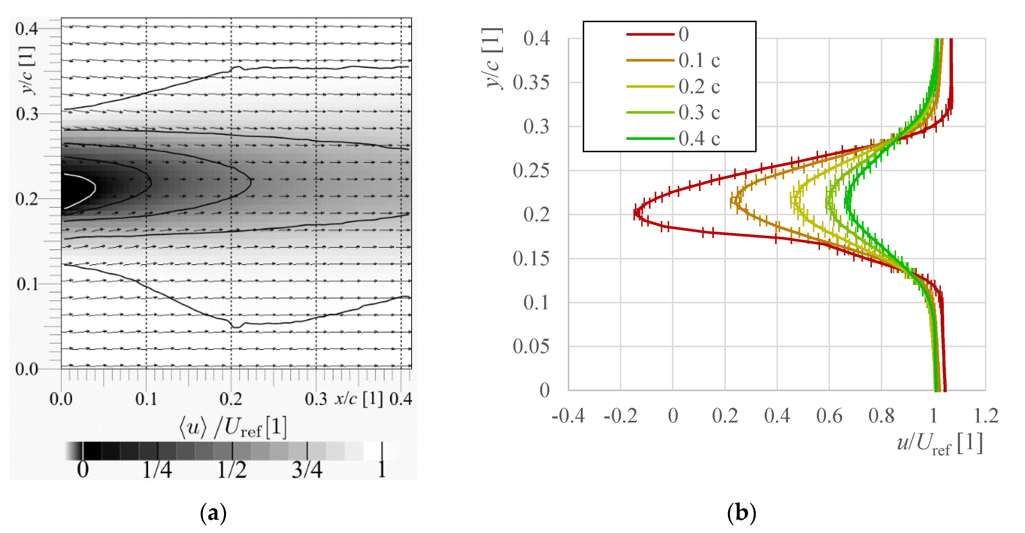
Figure 2.
Ensemble average stream-wise velocity. Panel (a) shows the map of average u (grayscale), the white isotach separates the area of back flow, the last black isotach separates the area of average velocity larger than reference velocity measured in empty wind tunnel. Panel (b) contains the velocity profiles at several distances from the trailing edge denoted as dashed lines in panel (a) distinguished via color: we apologize to readers with grayscale printer.

Figure 3.
(a) Wake width calculated according to the formulas for boundary layer thickness. The dash-dotted lines represent the calculation with constant , while the dashed line plays for usage of , which is the background of Gaussian fit and it develops with distance x. Dependence of these two velocities on x is displayed in panel (b).

Figure 4.
Panel (a) shows data at one of velocity profiles (Figure 2b) with corresponding Gaussian fit. There is shown the constant value of Uref, which is velocity measured in empty wind tunnel, and U0, which is the background of Gaussian fit. (b) The comparison of mentioned methods based on threshold (first four) or on the Gaussian fit (last two).

Figure 5.
Instantaneous stream-wise velocity. Panel (a) shows the map of u (grayscale) normalized by reference velocity. The white line represents the centers of Gaussian fits in transverse profiles, the pair of black lines are the centers plus/minus the σ-parameter of the fit. Panel (b) shows a single particular Gaussian fit at the stream-wise distance denoted as dashed line in panel (a).

Figure 6.
Panel (a) compares the wake width calculated as average of the instantaneous wake widths (Figure 5) with the wake width of ensemble-averaged stream-wise velocity by using the Gauss fit (black short-dashed line) and by using the threshold method (gray dashed line). The error bars represent the standard deviation of the instantaneous wake widths in each position. Panel (b) shows the position of wake centerline calculated on instantaneous (black solid line) or ensemble-averaged (gray dashed line) velocity field. Error bars are the standard deviation of the instantaneous wake positions.

Figure 7.
Standard deviation of stream-wise velocity. Panel (a) shows the map of σ(u) (grayscale) normalized by reference velocity. Panel (b) contains the standard deviation profiles at several distances from the trailing edge denoted as dashed lines in panel (a); we apologize to readers with grayscale printer.

Figure 8.
Standard deviation of stream-wise velocity. Panel (a) shows the map of σ(u) (grayscale) normalized by reference velocity. Panel (b) contains the standard deviation profiles at several distances from the trailing edge denoted as dashed lines in panel (a).
Figure 8.
Standard deviation of stream-wise velocity. Panel (a) shows the map of σ(u) (grayscale) normalized by reference velocity. Panel (b) contains the standard deviation profiles at several distances from the trailing edge denoted as dashed lines in panel (a).

Figure 9.
(a) Spatial distribution of stream-wise velocity flatness; the thick isoline refers to value of 3, the thin black isoline to 6, the white isoline to values greater than 12. (b) The instantaneous velocity field with value most different from the average in the point denoted by rectangle and a pair of arrows in bottom left corner. Note that this snapshot is a regular case, it is not noisier than the others, however there is some fluid of lower velocity ejected from the wake into the surroundings hitting the denoted point. (c) Spatial distribution of flatness of the ensemble without the snapshot (b). Note that removal of single case of 1208 significantly decreases the flatness signal in the denoted point.

Figure 10.
(a) Profiles of flatness coefficient of the stream-wise velocity component. (b) Profiles of the skewness of stream-wise velocity component at depicted distance past the trailing edge distinguished via colors: we apologize to readers with grayscale printer.
Figure 10.
(a) Profiles of flatness coefficient of the stream-wise velocity component. (b) Profiles of the skewness of stream-wise velocity component at depicted distance past the trailing edge distinguished via colors: we apologize to readers with grayscale printer.

Figure 11.
(a) Spatial map of the skewness of stream-wise velocity component. (b) Probability density function (PDF) of the instantaneous stream-wise velocities within the four denoted rectangles, solid line in the wake central region, dashed line in the inner shear layer (SL), dash-dotted line in the outer shear layer and the short, dashed line in the surrounding region. The u values are normalized by the local average and standard deviation. The inset shows the PDF as the function of velocity and it shows different widths and positions of the distributions (note the logarithmic scale in inset).

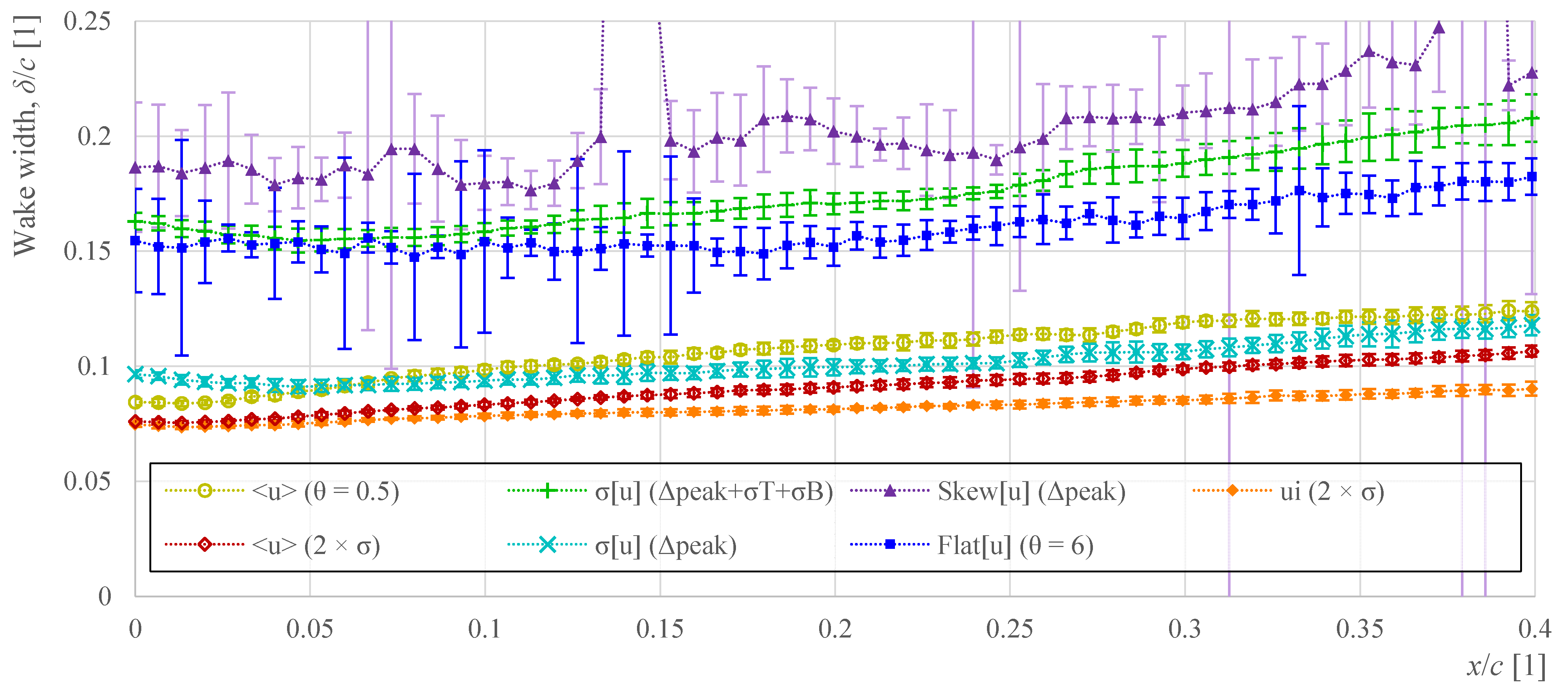
Figure 12.
Comparison of the discussed definitions of wake width past the airfoil NACA 64-618 at zero angle of attack. Horizontal axis is the distance past trailing edge; all lengths are normalized by the airfoil chord. Golden circles: the distance of points, where average velocity deficit crosses half (threshold θ = 0.5) the maximum velocity deficit. Maroon diamonds: twice the thickness σ of the Gauss function fitted to the average velocity profile. Orange diamonds: the average of wake widths fitted to each snapshot. Cyan Xs: the distance of double-Gauss peaks fitted to the profile of standard deviation of stream-wise velocity. Green crosses: distance of mentioned peaks plus the thicknesses of those peaks in the profile of standard deviation of stream-wise velocity. Violet triangles: distance of double-Gauss peaks fitted to the profile of stream-wise velocity skewness (third statistical moment). Blue rectangles: distance of points, where the stream-wise velocity flatness reaches the threshold θ = 6, i.e., 2 × 3, the Gauss reference value.

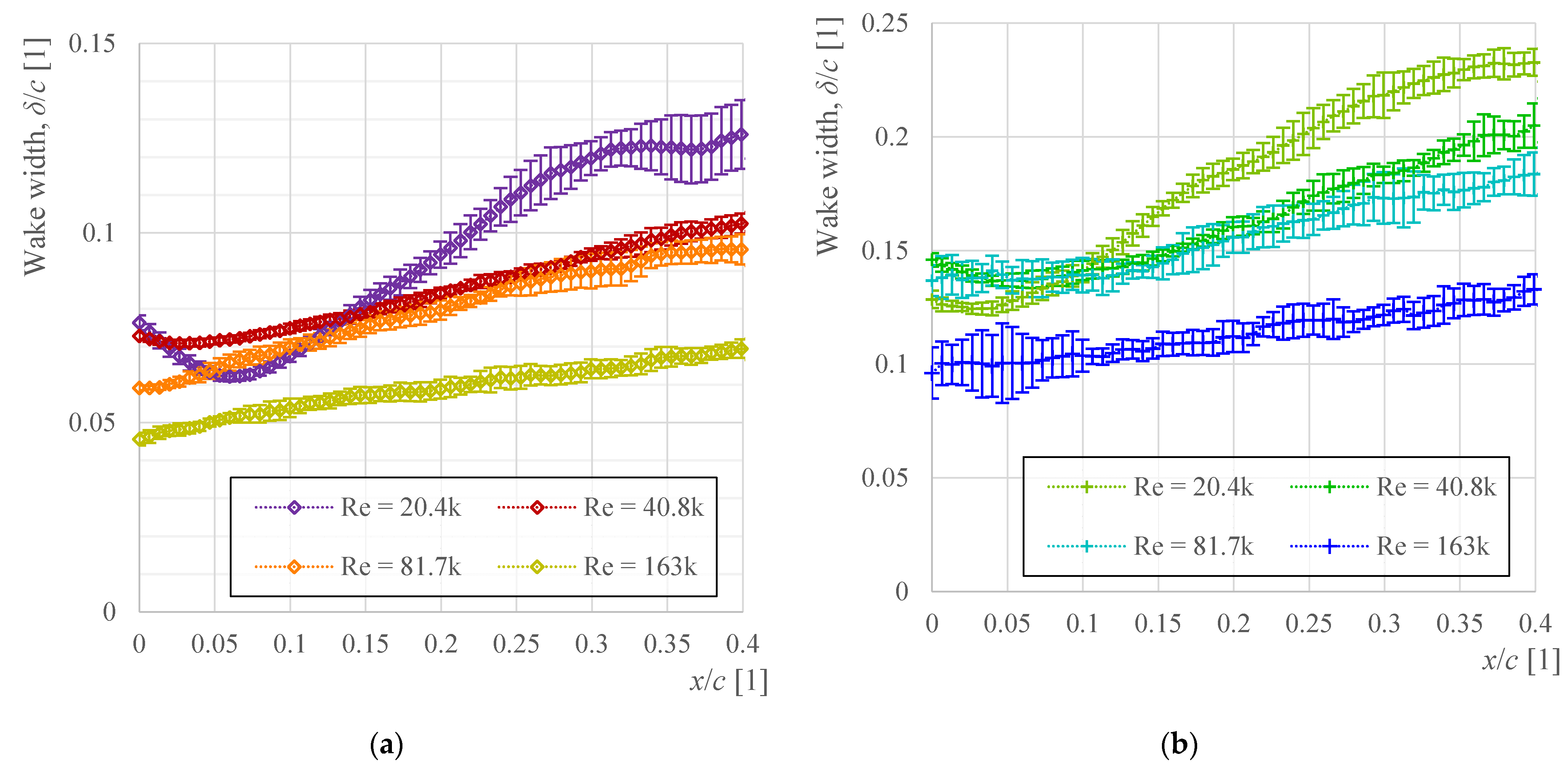
Figure 13.
Wake widths past airfoil at different Reynolds numbers (“k” denotes “·103”). Panel (a) shows the wake width calculated as the σ-parameter of Gaussian fit of the ensemble-averaged stream-wise velocity. Panel (b) shows the wake widths calculated by using standard deviation of stream-wise velocity fitted by double-Gauss function, the peak distance plus the width of bottom σB and top σT peak. Note the Re explored up to here is 6.1·104, it is not plotted here.

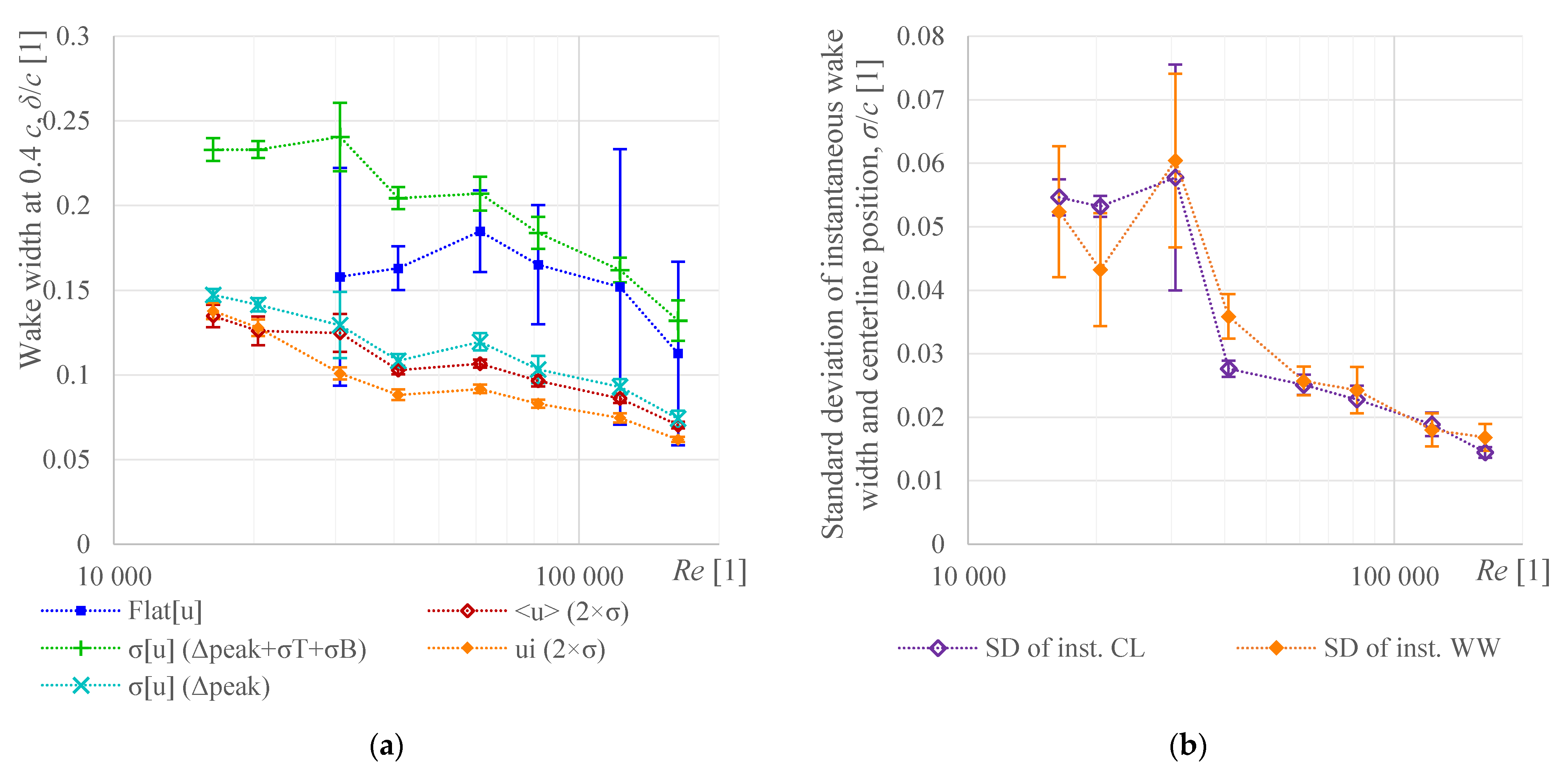
Figure 14.
(a) Comparison of possible wake width definitions at distance x/c = 0.4 past the airfoil NACA 64-618 trailing edge as a function of chord-based Reynolds number. Empty maroon diamonds denote the Gaussian fitting of average velocity profile, filled orange diamond the Gauss fitting of instantaneous velocity fields, the green crosses represent wake width based on peaks of stream-wise velocity standard deviation, cyan Xs represent the fluctuation peak distance only, and the blue squares represent the threshold of stream-wise velocity flatness, which fails for laminar flow, therefore, it is not plotted there. (b), Standard deviation of the instantaneous wake width calculated by using Gaussian fit (orange filled diamonds) and the standard deviation of the wake centerline position (violet empty diamonds), which can be interpreted as wake meandering.

Figure 15.
(a) Virtual origin x0 of the wake width, if its stream-wise development is approximated by linear function (8). The uncertainty of flatness-based wake width is so high that it is not plotted. (b) the grow rate a of the wake as a function of Reynolds number. The symbols are the same as in Figure 14.

Figure 16.
Wake widths at constant distance x/c = 0.4 as a function of number of snapshots used for averaging.
Figure 16.
Wake widths at constant distance x/c = 0.4 as a function of number of snapshots used for averaging.


Table 1.
The possible mathematical methods of extracting parameters of some data profile.
| Method | Advantages | Disadvantages |
|---|---|---|
| Threshold |
|
|
| Fitting |
|
|
Table 2.
The momenta of stream-wise velocity, which have been examined in this contribution.
| Moment of u | Advantages | Disadvantages |
|---|---|---|
| Average |
|
|
| Standard deviation |
|
|
| Skewness |
|
|
| Flatness |
|
|
Publisher’s Note: MDPI stays neutral with regard to jurisdictional claims in published maps and institutional affiliations. |
© 2021 by the authors. Licensee MDPI, Basel, Switzerland. This article is an open access article distributed under the terms and conditions of the Creative Commons Attribution (CC BY) license (https://creativecommons.org/licenses/by/4.0/).
Share and Cite
MDPI and ACS Style
Duda, D.; Uruba, V.; Yanovych, V. Wake Width: Discussion of Several Methods How to Estimate It by Using Measured Experimental Data. Energies 2021, 14, 4712. https://doi.org/10.3390/en14154712
AMA Style
Duda D, Uruba V, Yanovych V. Wake Width: Discussion of Several Methods How to Estimate It by Using Measured Experimental Data. Energies. 2021; 14(15):4712. https://doi.org/10.3390/en14154712
Chicago/Turabian StyleDuda, Daniel, Václav Uruba, and Vitalii Yanovych. 2021. "Wake Width: Discussion of Several Methods How to Estimate It by Using Measured Experimental Data" Energies 14, no. 15: 4712. https://doi.org/10.3390/en14154712
Note that from the first issue of 2016, this journal uses article numbers instead of page numbers. See further details here.