Joint Seismic and Gravity Data Inversion to Image Intra-Crustal Structures: The Ivrea Geophysical Body Along the Val Sesia Profile (Piedmont, Italy)
 Matteo Scarponi1*
  György Hetényi1
  Jaroslava Plomerová2
  Stefano Solarino3 Ludovic Baron1
  Benoît Petri4
- 1Institute of Earth Sciences, University of Lausanne, Lausanne, Switzerland
- 2Institute of Geophysics, Czech Academy of Sciences, Prague, Czechia
- 3Istituto Nazionale di Geofisica e Vulcanologia, DICCA Università di Genova, Genoa, Italy
- 4UMR7063, CNRS, Institut Terre et Environnement de Strasbourg, Université de Strasbourg, Strasbourg, France
We present results from a joint inversion of new seismic and recently compiled gravity data to constrain the structure of a prominent geophysical anomaly in the European Alps: the Ivrea Geophysical Body (IGB). We investigate the IGB structure along the West-East oriented Val Sesia profile at higher resolution than previous studies. We deployed 10 broadband seismic stations at 5 km spacing for 27 months, producing a new database of ∼1000 high-quality seismic receiver functions (RFs). The compiled gravity data yields 1 gravity point every 1–2 km along the profile. We set up an inversion scheme, in which RFs and gravity anomalies jointly constrain the shape and the physical properties of the IGB. We model the IGB’s top surface as a single density and shear-wave velocity discontinuity, whose geometry is defined by four, spatially variable nodes between far-field constraints. An iterative algorithm was implemented to efficiently explore the model space, directing the search toward better fitting areas. For each new candidate model, we use the velocity-model structures for both ray-tracing and observed-RFs migration, and for computation and migration of synthetic RFs: the two migrated images are then compared via cross-correlation. Similarly, forward gravity modeling for a 2D density distribution is implemented. The joint inversion performance is the product of the seismic and gravity misfits. The inversion results show the IGB protruding at shallow depths with a horizontal width of ∼30 km in the western part of the profile. Its shallowest segment reaches either 3–7 or 1–3 km depth below sea-level. The latter location fits better the outcropping lower crustal rocks at the western edge of the Ivrea-Verbano Zone. A prominent, steep eastward-deepening feature near the middle of the profile, coincident with the Pogallo Fault Zone, is interpreted as inherited crustal thickness variation. The found density and velocity contrasts of the IGB agree with physical properties of the main rock units observed in the field. Finally, by frequency-dependent analysis of RFs, we constrain the sharpness of the shallowest portion of the IGB velocity discontinuity as a vertical gradient of thickness between 0.8 km and 0.4 km.
Introduction
The geologically defined Ivrea-Verbano Zone (IVZ) and the related but much longer Ivrea Geophysical Body (IGB) belong to the most outstanding features of the whole Alpine domain. They have been the subject of numerous international investigations in the fields of geology, petrology and geophysics (e.g., Schmid et al., 2017; Petri et al., 2019; Kissling et al., 1984 and detailed references below).
The western end of the Southern Alps (Figure 1A) is regarded as a nearly complete cross-section of the continental crust, exposing upper to middle and middle to lower crustal composition rocks at its surface in the Serie dei Laghi and the IVZ, respectively (e.g., Fountain, 1976; Khazanehdari et al., 2000). These units belong to a complex tectonic setting, which has been mapped by several groups of authors (e.g., Schmid et al., 2004; Brack et al., 2010; Petri et al., 2019).
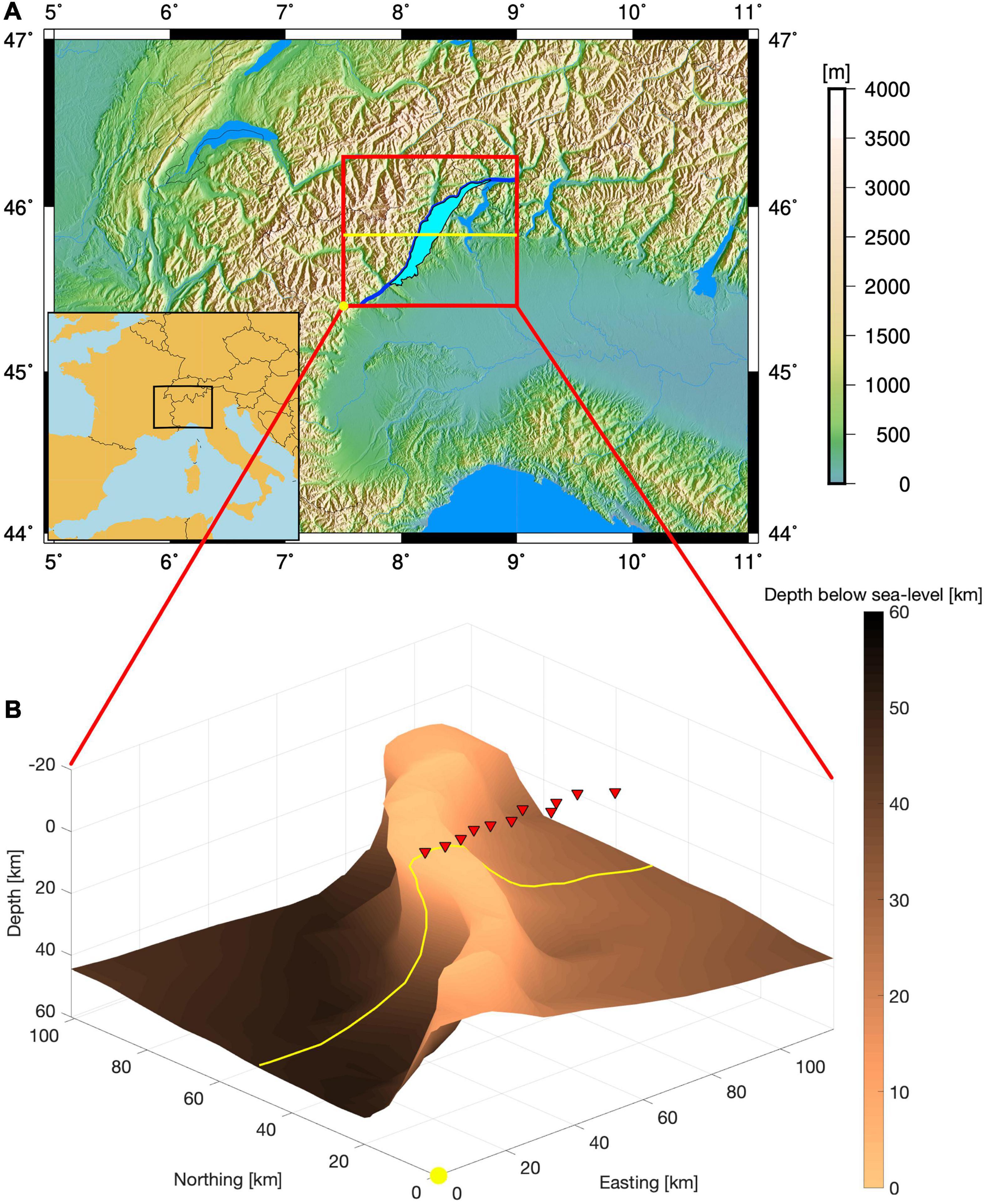
Figure 1. Study area and earlier 3D IGB density model. (A) View of the study area. The 2D cross-section investigated in this study, along the 2D West-East IvreaArray seismic profile (red triangles in panel b), is highlighted by a yellow line. This target profile extends across the IVZ (cyan shape), delimited on the West by the Insubric Line (blue line). The yellow circle is the origin of the km-coordinate system used in this study and the subsequent figures (7.5°E, 45.4°N). The inset show the overview map’s location in Europe. (B) Perspective view of the IGB 3D density model interface, constrained by gravity data modelling in an earlier study (Scarponi et al., 2020).
This work focuses on the IGB, which constitutes the crustal root of the IVZ and consists of an anomalously dense and seismically fast rock complex. This anomalous crustal complex extends along the whole inner arc of the Western Alps and outcrops in its north-eastern portion as the IVZ. The IGB is nowadays regarded as a sliver of the Adriatic lower lithosphere (e.g., Schmid et al., 2017; Petri et al., 2019), which was involved in the Alpine collision and tectonically emplaced at unusual shallow depths (e.g., Handy et al., 2015). The Adriatic plate, among other micro-plates, was one of the key actors in the Alpine collision and the related orogenic process, which featured the subduction of the former Tethys ocean and the subsequent Adriatic thrusting against the European margin (e.g., Handy et al., 2010).
The IGB is associated with pronounced seismic, gravity and magnetic anomalies (e.g., Lanza, 1982; Kissling et al., 1984; Diehl et al., 2009). The IGB is bounded by the Western Alps along the Insubric line (IL): a main vertical to sub-vertical fault line (Schmid et al., 1987, 1989; Berger et al., 2012) which separates the Adriatic plate from the orogenic wedge (Figure 2A).
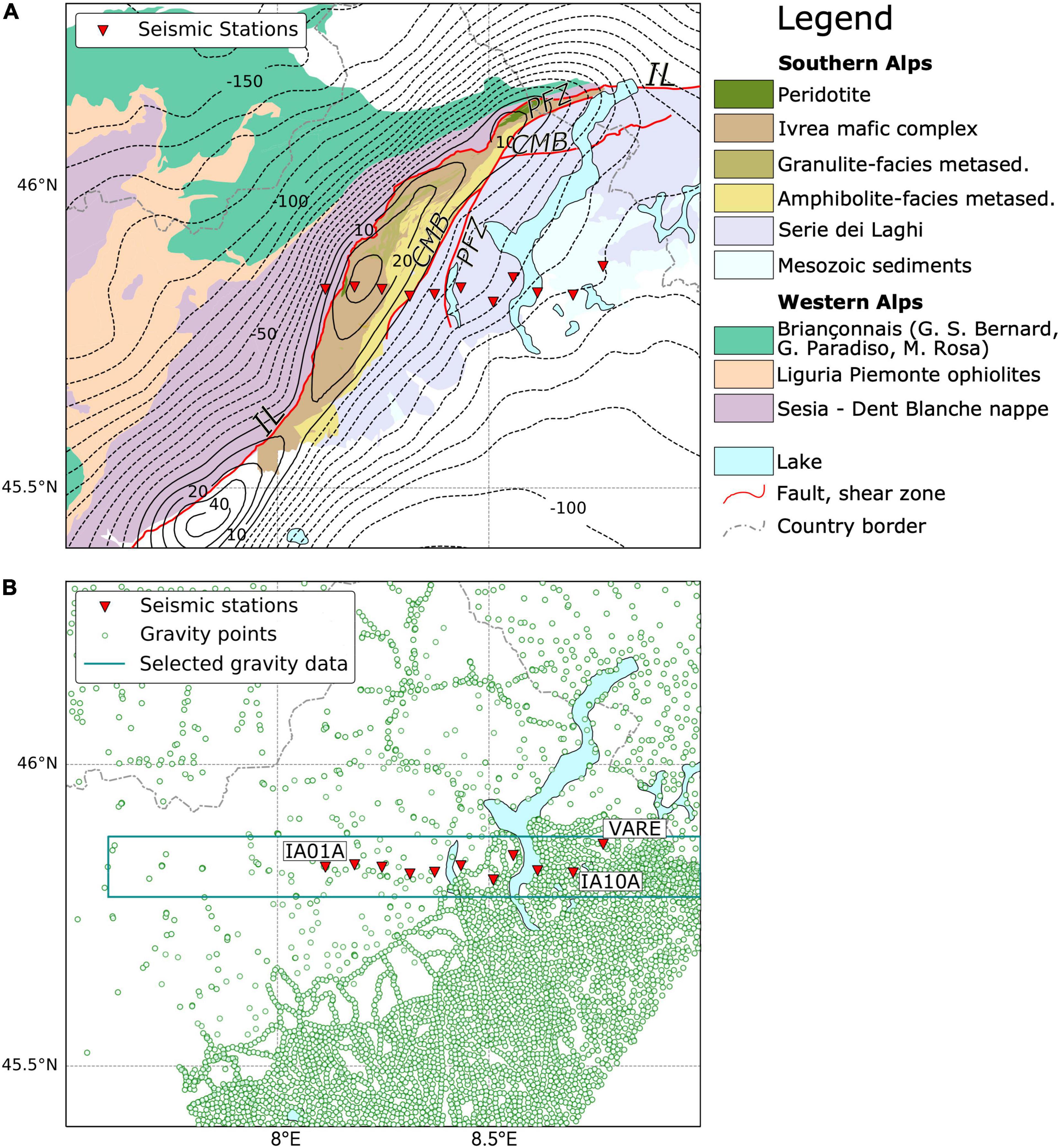
Figure 2. (A) Geological map of the IVZ and the surrounding areas, simplified from Petri et al. (2019) and Schmid et al. (2004) (see legend on the right hand of the figure), together with the location of the 10 IvreaArray broadband seismic stations and the INGV permanent seismic station IV.VARE [red triangles, see station names in (B)]. The main faults (red lines), relevant for this study, are indicated as “IL” for Insubric Line, “PFZ” for Pogallo Fault Zone and “CMB” for Cossato-Mergozzo-Brissago Line. Overlaid, the 10 mGal contour lines for the Bouguer gravity anomaly from our data across the study area. (B) The compiled gravity data set for this study is shown (green circles), which comprises earlier existing gravity data and recently collected gravity data in the scope of the work of Scarponi et al. (2020). The location of the IvreaArray seismic stations is shown (red triangles) together with the INGV permanent seismic station IV.VARE and their names. The cyan box indicates the gravity data we selected for this study along the 2D IvreaArray profile. The dashed-pointed gray line indicates the Swiss-Italian border as shown in the legend.
A long history of investigations has addressed the IGB, both in terms of gravity mapping (e.g., Niggli, 1946; Vecchia, 1968; Masson et al., 1999) and gravity data modeling, with models based on continuous bodies with a sharp and constant density contrast (e.g., Berckhemer, 1968; Kissling et al., 1984), and on heterogeneous-size and -density blocks as well (e.g., Bayer et al., 1989; Bürki, 1990; Rey et al., 1990). Concerning seismic investigations, the IGB was first imaged by refraction experiments (Berckhemer, 1968; Ansorge, 1979), which lead to the birth of an iconic model, usually referred to as the “Bird’s Head” in the literature. This became of historical value with subsequent investigations, revealing high level of structural complexities of the IGB (e.g., Ansorge, 1979). In the frame of the ECORS-CROP experiment, the regional crustal structure was investigated via reflection seismics (e.g., Bayer et al., 1989; Nicolas et al., 1990; Thouvenot et al., 1990), guiding the development of several 2D gravity models but also stressing the limitations of controlled-source seismology, in imaging such a complex structure as the IGB (Kissling, 1993). Local earthquake analysis and tomography (LET) studies (e.g., De Franco et al., 1997; Diehl et al., 2009; Solarino et al., 2018) allowed the IGB to be better imaged and interpreted in light of the tectonic setting as well (Schmid and Kissling, 2000). Despite the latest advances in the terms of LET resolution (Diehl et al., 2009 provides the crustal vP structure on a 25 × 25 × 15 km grid and Solarino et al., 2018 locally higher, up to 15 × 15 × ∼ 10 km), a spatial imaging gap persists between the IGB structure at the geological maps’ spatial scale. Therefore, structural questions on the IGB’s relation with the exposed IVZ remain open.
Recent gravity investigations, based on new, densely spaced gravity surveys and earlier-existing compiled gravity data (Figure 2B) allowed the development of a new 3D IGB gravity model across the IVZ area (Scarponi et al., 2020) and (Figure 1B). In this work, we focus on a central cross-section of this most recent 3D IGB model (Figure 1B) and we integrate the gravity dataset with new high-resolution broad-band passive seismic data, recorded during the IvreaArray passive seismic experiment (Hetényi et al., 2017). We intend to use the new seismic data to further constrain the most recent IGB 3D density model along the IvreaArray profile (Figure 2B). In fact, we investigate the West-East oriented 2D profile along Val Sesia (∼ 45.83°N), crossing the entire IVZ at that latitude (∼ 8.11°E to 8.77°E). We model the IGB along this 2D cross-section as a body below a single discontinuity, and set up a joint inversion scheme to fit the observed gravity anomaly and seismic receiver functions (RFs) from IvreaArray, to constrain both the shape and the physical properties of the IGB. The RF technique enhances smaller-amplitude P-to-S (Ps) converted phases in the P-wave coda, and extracts information on the Earth discontinuities beneath a seismic receiver (Langston, 1979). While RF inversion is routinely performed to investigate the seismic properties of the crust and the upper mantle (Bodin et al., 2012), inverting the RFs-only is in general a strongly non-linear and non-unique problem (Ammon et al., 1990). Joint inversions of RFs along with complementary geophysical observations reduce this non-uniqueness. Such complementary data sets can be, e.g., RFs and surface wave dispersion curves (Julia et al., 2000), also with the addition of magnetotelluric data (Moorkamp et al., 2010) or RFs combined with gravity data and seismic tomography (Basuyau and Tiberi, 2011).
Here, we implement a novel iterative joint inversion algorithm, acting on the gravity and seismic data. This algorithm is meant to explore and characterize the performance of all considered IGB models in non-probabilistic terms, by implementing a performance-driven pseudo-random walk in the model space. The gravity anomaly along the profile and the computed seismic RFs represent our observations. In particular, we combine the sensitivity of gravimetry to the geometry and magnitude of density contrasts in the subsurface structure, with the sensitivity of RFs to the crustal discontinuities beneath the seismic receiver.
Data and Data Products
New seismic data has been acquired and recent gravity data has been compiled to produce a higher resolution image of the IGB along the Val Sesia profile. The following paragraphs present how the data was obtained and processed prior to the joint inversion. The complete seismic dataset is directly available in the Supplementary Material, in the form of radial (RRF) and transverse (TRF) seismic receiver functions.
The IvreaArray Seismic Network
We collected the new seismic data in the framework of IvreaArray (Hetényi et al., 2017): a temporary seismic network, installed and operated for 27 months (June 2017 to September 2019) as one of the AlpArray complementary experiments.
The main purpose of IvreaArray was to record high-quality seismic signals at a higher spatial resolution in Val Sesia, compared to earlier studies addressing the crustal structure in the Western Alps and in the IVZ.
For this purpose, we deployed 10 broadband three-component seismic stations at 5 km spacing along a West-East linear profile (∼ 45.83°N). The INGV permanent seismic station IV.VARE is included as it located as a natural eastern continuation of IvreaArray (Figure 2B). All 10 deployed sensors were the Güralp CMG-3ESP seismometers of the Czech MOBNET pool, with 60 s lower corner frequency. The linear seismic profile crosses the entire IVZ. It starts few km to the west of the IL at ∼ 8.11°E (in the village of Boccioleto), then crosses the lower and middle crustal rocks outcropping in the IVZ and extends to the eastern shore of Lago Maggiore (∼ 8.77°E).
The seismic network operated for 27 months and continuously recorded data at 100 Hz sampling rate on all three components. Data recovery was ∼ 90%. During this time and according to the USGS earthquake catalog, we selected and retrieved 347 events of interest for our study (magnitude ≥ 5.4, epicentral distance 28°≤ Δ ≤ 95°, Supplementary Material 1).
Seismic Receiver Functions
We process the recorded teleseismic signals by computing seismic receiver functions: a deconvolution-based technique which enhances the arrival of P-to-S (Ps) converted phases (Langston, 1979). Ps converted phases follow the direct P-wave arrivals. They are produced when an impinging P-wave encounters a discontinuity – an impendence contrast – in the propagating medium beneath a seismic receiver, thus containing information on the associated Earth structure. A receiver function is mathematically defined as the deconvolution of the seismogram’s vertical component from the radial component, yielding a series of delay times with respect to the first P-wave arrival (Langston, 1979). This operation removes the event source time function and the distant-path effects from the trace, favoring a constructive stacking to investigate the receiver side Earth structure. The analysis of the Ps delay times and amplitudes carries information on the depth of a seismic discontinuity and the shear-wave velocity vS profile, together with the magnitude of the impedance contrast itself, with a primary sensitivity for the vS contrast.
We compute RFs based on the time-domain iterative deconvolution technique (Ligorría and Ammon, 1999) by iteratively cross-correlating the vertical and the horizontal (radial) seismic traces and saving the associated delay times, generated by the strongest amplitudes first and by the minor ones later on. The final RF is obtained via convolution of the spike train with a Gaussian pulse, whose width corresponds to the maximum allowed frequency into the seismic signal during pre-filtering (see RRF and TRF in Supplementary Material).
In our case, we filtered the seismic data in the 0.1 Hz to 1 Hz frequency band and performed 150 iterations during deconvolution for each RF. Quality control (QC) is applied both on the seismic traces and on the final RFs. First, we look for amplitude similarity for each seismogram component across all the stations for each seismic event, and for teleseismic signal prominence with respect to the background noise. Then, for each computed RF, we verify an acceptable location of the reference direct-P wave signal and for its satisfactory recovery in terms of amplitude. We refer the reader to the work (e.g., Hetényi et al., 2015, 2018; Subedi et al., 2018) for further description of this QC practice. This ensured retrieval of high-quality earthquake signal (in the original seismogram components) and of the direct-P arrival (in the computed RF) prior to the converted phases, providing a final dataset of ∼ 1000 high-quality RF traces. The original seismic traces were rotated into the LQT, ray-based coordinate system. This practice allows us to maximize the Ps amplitude and to prevent the direct-P signal from strongly interfering with the peaks’ interpretation in case of very shallow interfaces, which are expected in the IVZ. The distribution of all available RFs shows a strong variability in the peak polarities and delay times as a function of the back-azimuth (Supplementary Material 2), in particular between the traces coming from the East and the West, which hints at the presence of dipping interfaces. In fact, dipping interfaces and/or anisotropic layers can affect the signal polarity and introduce back-azimuthal periodicities, especially on the transverse RF component (e.g., Levin and Park, 1997). By inspecting all the transverse RF signals from the IvreaArray recordings (see TRF in Supplementary Material), we could find some but limited evidence for local dipping structures, but no clear signs of resolvable anisotropy at any of the stations, and therefore decided not to address this particular feature in the subsequent analysis.
Relative to the RF complexity, reverberations cause so-called multiples and small-scale heterogeneities can increase noise. Furthermore, as RFs record delay times, there is a trade-off between layer thickness and average vP/vS, which prevents from uniquely inverting for the Earth structure by using RFs Ps phases only (e.g., Ammon et al., 1990).
To address these limitations, and to avoid stacking numerous waveforms sampling a heterogeneous crust in the IVZ, we migrate the observed RFs from time to depth and produce migrated profiles. During migration, we perform ray-tracing for each station–event pair with a vertical resolution of 0.25 km using a 2D velocity model and respecting Snell’s law including local interface dip. Then we distribute the RF time sample amplitudes along these ray paths to finally obtain a migrated image, with a final spatial resolution of 0.5 km. The migration spatially re-distributes wave conversions to where they were produced, and gives a structural image of the sub-surface. The areas where the RF amplitudes are stacked constructively represent either an increase or a decrease of seismic velocity with depth. Figure 3B shows an example for the 1D iasp91 velocity model (Kennett and Engdahl, 1991).
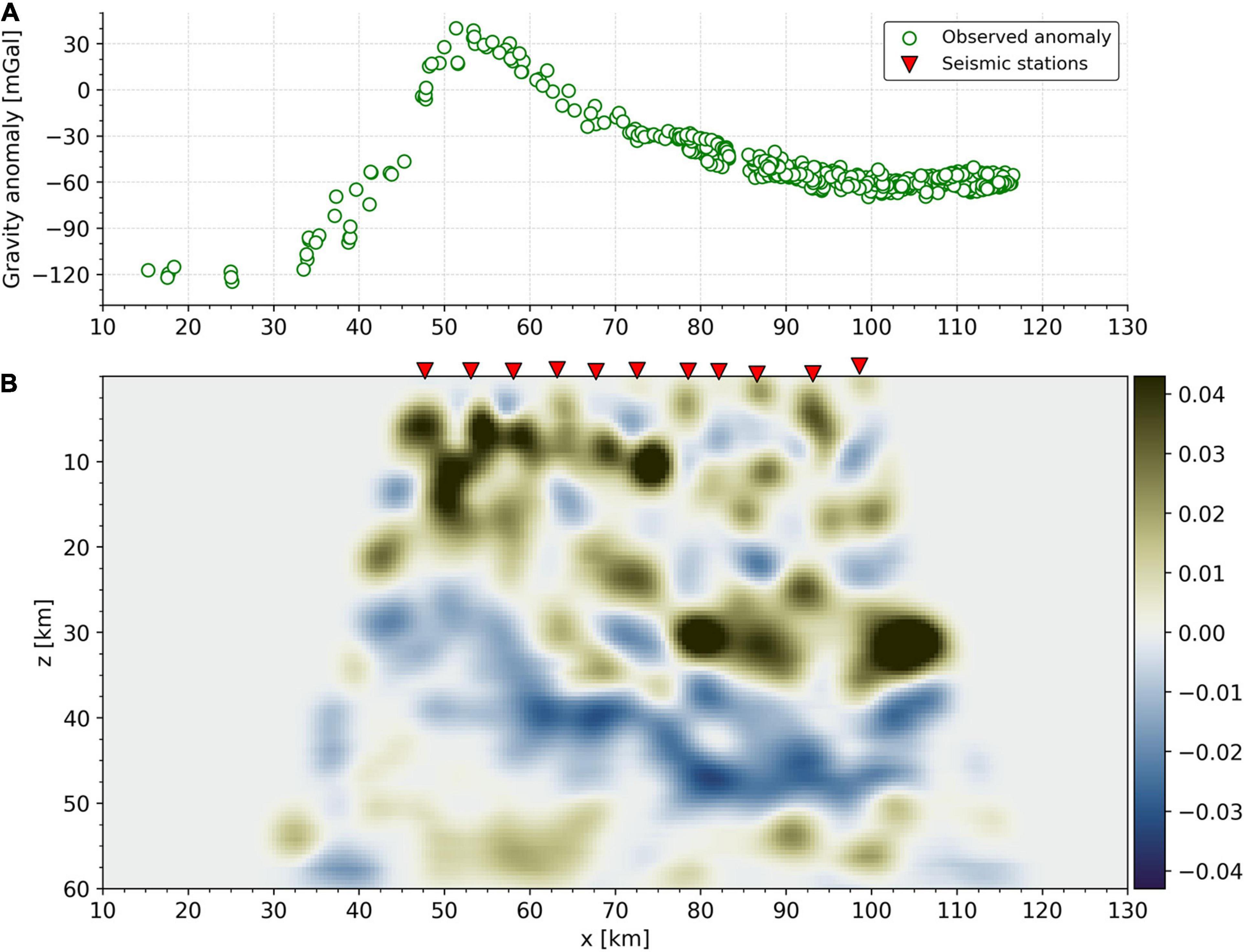
Figure 3. (A) Niggli gravity anomaly computed from observed data and applying rock-density-based terrain corrections (Scarponi et al., 2020) along the West-East IvreaArray profile. (B) An example of migrated receiver function profile with the use of the IvreaArray and VARE seismic data and the iasp91 velocity model for ray-tracing and migration. Colors highlight areas of increasing (brown) and decreasing (blue) seismic velocities with depth.
While the observed RFs constitute the seismic part of the input to the joint inversion scheme, the computation of RF migration images is incorporated into the iterative inversion procedure, and constitutes the actual mean for the model seismic performance evaluation. The detailed description of the inversion workflow is provided in section “Inversion Approach.”
Gravity Anomalies Along Val Sesia
We compiled a gravity dataset by merging earlier and the most recent gravity data acquired across the IVZ. The earlier existing gravity data points were compiled from the Swiss Federal Office of Topography (Swisstopo)1 and from the Istituto Nazionale di Oceanografia e di Geofisica Sperimentale (OGS)2, and were merged with the most recent data set in our earlier work (Scarponi et al., 2020). The full dataset was analyzed in the same work (Scarponi et al., 2020), where the original raw relative gravity measurements were processed and transformed into absolute gravity values with the software GravProcess (Cattin et al., 2015), with a final mean uncertainty of 0.22 mGal (1 Gal = 1 cm/s2). The reader is referred to the work of Scarponi et al. (2020) for full details of the gravity data acquisition practices and processing. In our joint inversion, we use a subset of this data (Figure 2B). The compiled dataset reaches a coverage of 1 gravity point every 1 to 2 km along the Val Sesia profile. For the joint inversion presented here, we include all the gravity points up to 5 km to the North and to the South along the IvreaArray seismic profile (Figure 2B). As the gravity data points were not uniformly distributed along the IvreaArray profile, we binned the data at 2 km intervals along the profile, obtaining a more balanced spatial distribution and allowing for faster gravity data modeling (0.08s instead of 1s for each test model). For each interval, the considered gravity data points were averaged in location (x and z coordinates) and in the measured gravity anomaly, with mean standard deviation of 3 mGal across the whole profile (Supplementary Material 5).
The final gravity data product we use in the inversion of this study is the Niggli gravity anomaly, which is an improved Bouguer anomaly considering surface rock densities for the terrain and plate corrections (Scarponi et al., 2020). This anomaly is obtained by the classical correction of the absolute gravity values for the effect of homogeneous and constant-density 3D topographical masses (i.e., Bouguer plate correction and terrain correction with ρ = 2670 kg/m3), accounting for the density variations of rocks seen at the surface and extrapolated down to sea-level (i.e., the Niggli correction), which is well justified by the general IVZ vertical structure (e.g., Fountain, 1976; Khazanehdari et al., 2000).
Considering the Niggli gravity anomaly (henceforth simply gravity anomaly) as final gravity observation allows us to focus our modeling effort on the IGB crustal structure below sea level and to analyze it consistently together with seismic RF migration images (Figure 3).
Inversion Approach
To reduce the non-uniqueness of RF-only inversion (Ammon et al., 1990), which are sensitive to sharp discontinuities, we jointly invert them with the gravity data, which are sensitive to volumetric anomalies. The RF inversion task has been addressed by many authors in the literature with the application, among others, of different algorithms such as: genetic algorithm (e.g., Shibutani et al., 1996; Levin and Park, 1997), simulated annealing (e.g., Vinnik et al., 2004) and neighborhood algorithm (e.g., Sambridge, 1999). The reader is referred to (Bodin et al., 2012) for further discussion on RF inversion approaches.
For this joint gravity and seismic data inversion, we implemented an iterative algorithm to explore the ensemble of all possible IGB models (i.e., the model space) and to evaluate their performance in terms of their fit to the observations. Even at a simplified parameterization of the model, the high dimension of variables (9 in our case) can require long and computationally expensive efforts (Sambridge and Mosegaard, 2002). To extract more information on models’ behaviour in an efficient manner, our iterative algorithm explores in a guided pseudo-random fashion the model space. The algorithm is based on the principles of a Monte Carlo exploration, as at each iteration a new candidate model is proposed upon a random perturbation of the current model, and the exploration evolves as a series of small random steps. Strictly speaking, we implemented a Markov chain property as well, as the candidate model depends only on the current model, and its acceptance is based on the performance of its forward model with respect to the current’s one only. If the new candidate model presents a better fit to the data (i.e., the performance), it is always accepted. Otherwise, its acceptance depends on a probability: the poorer the performance, the lower the chance to be accepted.
At each iteration, the evaluation of the overall performance for a given candidate model consists of two parts – the seismic and gravity data modeling, respectively – which are eventually combined together upon comparison with the seismic and gravity observations (Figure 4). It develops as follows. Given a candidate model, the associated velocity structure (defined by the candidate IGB model geometry, velocity and density contrasts) is used for both the seismic ray-tracing, and the computation and migration of the synthetic RFs. The same velocity structure and the associated ray-tracing are subsequently used for the migration of the observed RFs. We thus obtain a “synthetic” and an “observed” RF migration image, respectively, which are then compared to define the candidate model’s seismic performance. Similarly, the gravity model performance is evaluated by comparing the observed gravity anomaly to the synthetic gravity anomaly, computed for the same candidate model structure (Figure 4). The following paragraphs discuss more in detail the model parameterization, the associated forward problem solution and joint model performance definition, and the technical implementation of the model space exploration.
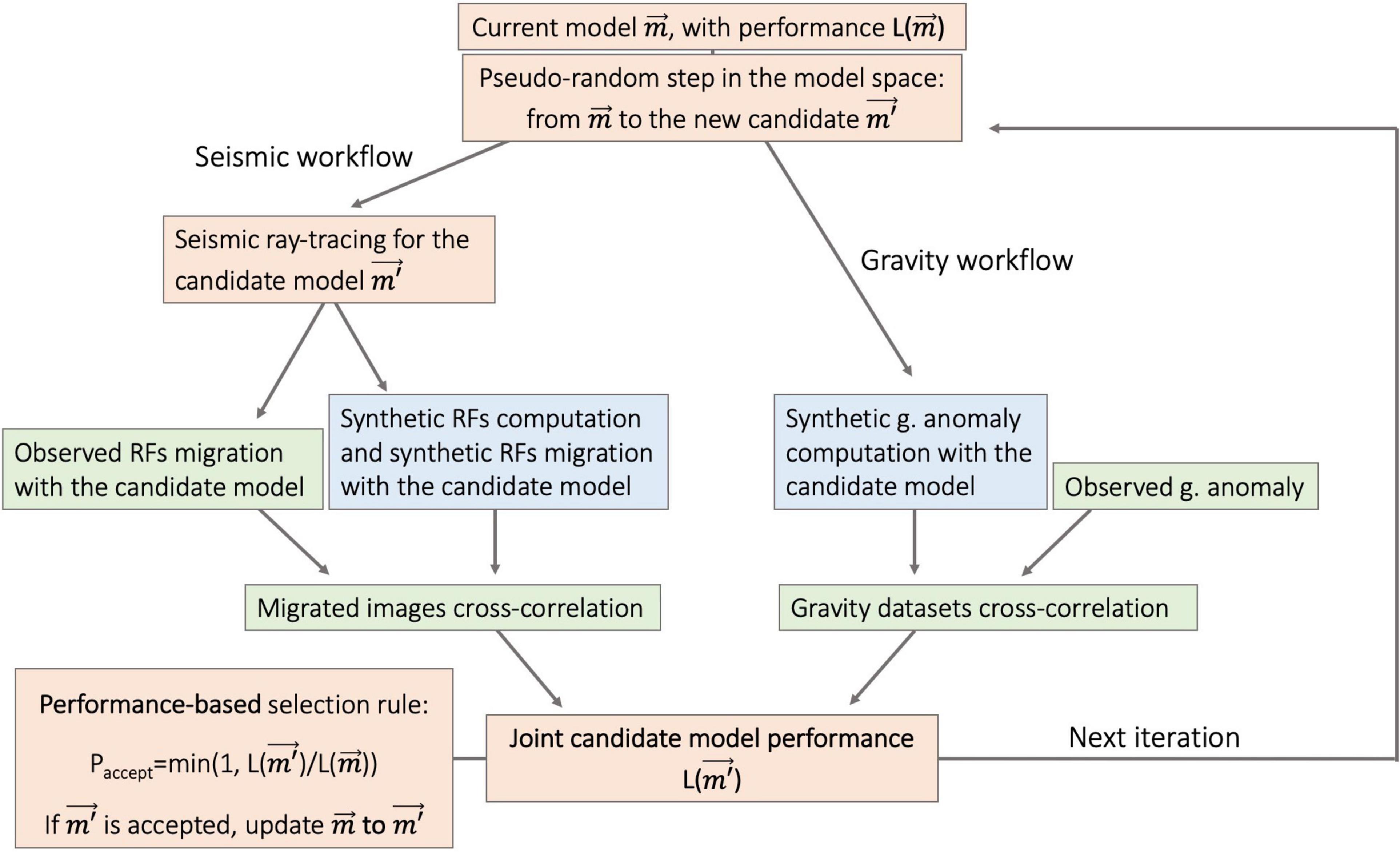
Figure 4. The joint seismic-gravity inversion workflow implements a performance-driven pseudo-random walk in the model space and a performance-based selection rule for the new candidate models. Red boxes refer to the new candidate model generation and evaluation, followed by the forward modeling steps (blue boxes) and by the model performance evaluation (green boxes). At each iteration, a new candidate model is proposed. Successively, the associated seismic and gravity model performances are evaluated and combined into a joint model performance, which determines whether the newly proposed model is accepted or not (following the idea behind the Metropolis-Hastings selection rule). For coherency, the same model is used both for migrating the observed RFs and for generating and migrating the synthetic RFs at each step. The iterative procedure continues by suggesting new model space samples until the maximum number of iterations is reached.
Model Parameterization
We model the IGB’s upper boundary as a single 2D discontinuity with a few segments, associated with sharp density (δρ) and shear-wave seismic velocity (δvS) contrasts (Figure 5) representing the IGB bulk physical properties with respect to the surrounding crust. While the former parameters are allowed to vary independently during the inversion, a homogeneous crustal background is assigned to the model and characterized by absolute values of vS = 3.5 km/s and density = 2700 kg/m3, which is also a consistent choice of velocity and density values, according to the vS-density relationship from Brocher (2005) (as further discussed in section “Results”). The choice of the background velocity fits well the upper crustal layer properties of 3.6 ± 0.2 km/s deduced from a short period regional network (De Franco et al., 1997). The vP/vS ratio is fixed at 1.73 and 1.8 for the medium above and below the model interface, as indicated by the iasp91 model for the upper and lower crustal rocks. The number of parameters has been chosen based on the a priori knowledge of the IGB and of the associated seismic and gravity anomalies. (Berckhemer, 1968) and (Kissling et al., 1984) provided seismic and gravity evidence for an anomalously dense, eastward-dipping body. Further contributions showed sub-vertical and eastward-dipping units to the East of the Insubric Line (e.g., Zingg et al., 1990; Petri et al., 2019). In addition, the preliminary RF migration with a 1D velocity model (Figure 3) clearly points to a shallow interface in the western portion of the profile, and a deeper interface further to the East. In our investigation of the shape of the IGB-top structure, the model boundaries connect to the eastern and the western branches of the regional Moho interface (Spada et al., 2013), acting as far-field constraints on either side of our study’s imaging area. We selected this Moho map as the reference crustal thickness only outside our data coverage and modeling domain, and kept it unvaried during the inversion procedure. The IGB model geometry is parameterized by 4 nodes, whose location can vary in space within given boundaries. This allows for a complete exploration in terms of width and depth of IGB head and neck, in analogy with the historical bird model anomaly as a vertical protuberance reaching shallow depths. The locations of the nodes, connected by straight segments, define the IGB model structure within the investigation domain (Figure 5). The western connection between node 1 and the Moho mimics the curved shape obtained in the 3D gravity model (Scarponi et al., 2020), as such a steep boundary is not resolvable with converted seismic waves.
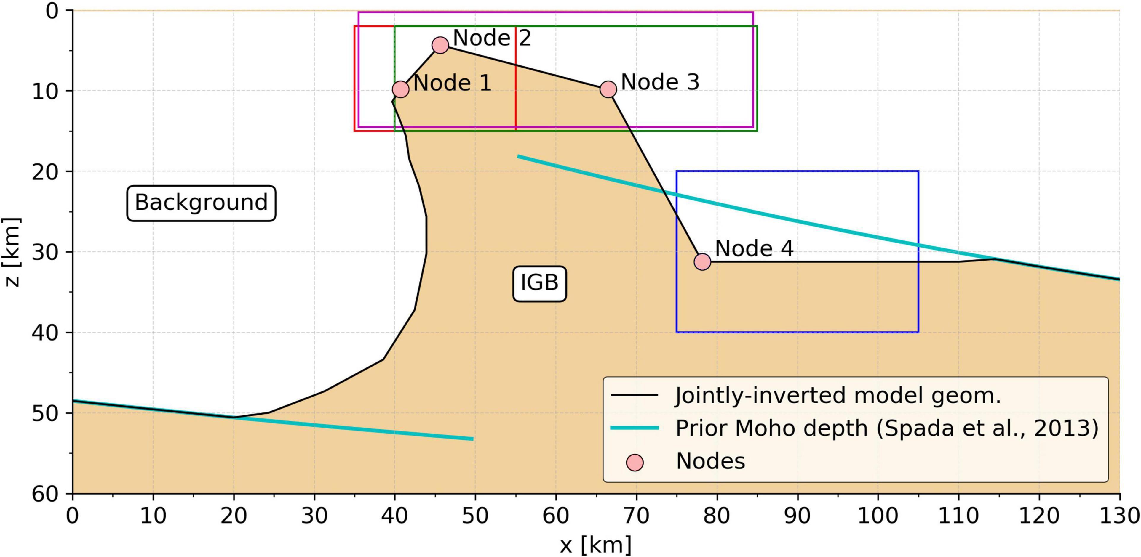
Figure 5. Model parameterization of the IGB shape used for the joint inversion of seismic and gravity data. We invert for the 2D IGB interface geometry (black line), whose configuration depends on the coordinates of four nodes (red, magenta, green, and blue). Spatial positions of each node are investigated within a given perimeter (dashed boxes of respective color) during the inversion, together with the velocity and density contrast of the IGB relative to the surroundings. The far-field model geometry connects to the Moho map (Spada et al., 2013). In the East, the connection is by a horizontal line. In the West, the curved shape is taken from the earlier 3D gravity model of (Scarponi et al. (2020)), as the vertical wall cannot be resolved by converted seismic waves.
We hence expect a shallow, not necessarily flat, discontinuity in the western portion of the profile and an eastward dipping structure – at an undetermined angle – toward the eastern portion of the profile. Therefore, we define four nodes to determine the IGB model geometry, and we prescribe that the depth of node 3 is the same as the depth of node 1. This still allows accounting for the East-West extent of the IGB, its variable eastern slope (due to the relative position of nodes 2 and 4), as well as a shallow interface with two segments, but saves one parameter to invert for.
Then, each IGB model is completely defined by 9 parameters:
All these parameters can attain values within a fixed range, with the exception of z2 and x2, as node 2 is always prescribed to be located between (along x) and above (along z) node 1 and node 3, in order to investigate the shallowest features of the IGB head. Similarly, node 4 is prescribed to be farther east than node 3. Therefore, the allowed value ranges for x2, z2 and x4 are dynamically adapted at each iteration, depending on the other parameter values. Figure 5 summarizes the possible range for each of the 9 inverted parameters, with minimum and maximum values based on a priori geometry and rock properties. The allowed range ofδρ (Table 1) is broader than that of the best fit 3D gravity model (400 ± 100 kg/m3, obtained by sensitivity analysis in Scarponi et al., 2020), while the range of δvS allows changes in a very broad range with respect to lower crust to mantle vS change in iasp91 (0.72 km/s). It also includes the full range of velocity variations from upper crust to upper mantle (up to 4.8 km/s) as suggested by the short-period regional network (De Franco et al., 1997).
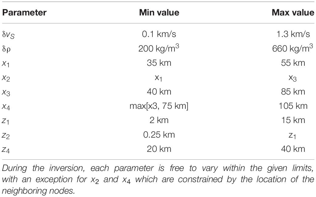
Table 1. Allowed-values range for each of the model space parameters.
Forward Calculation and Model Performance
The forward modeling task produces the synthetics to be compared with the respective observations, for a given candidate model. It consists of two separate contributions – the seismic and the gravity part – whose misfits are then combined (see Figure 6 for an example).
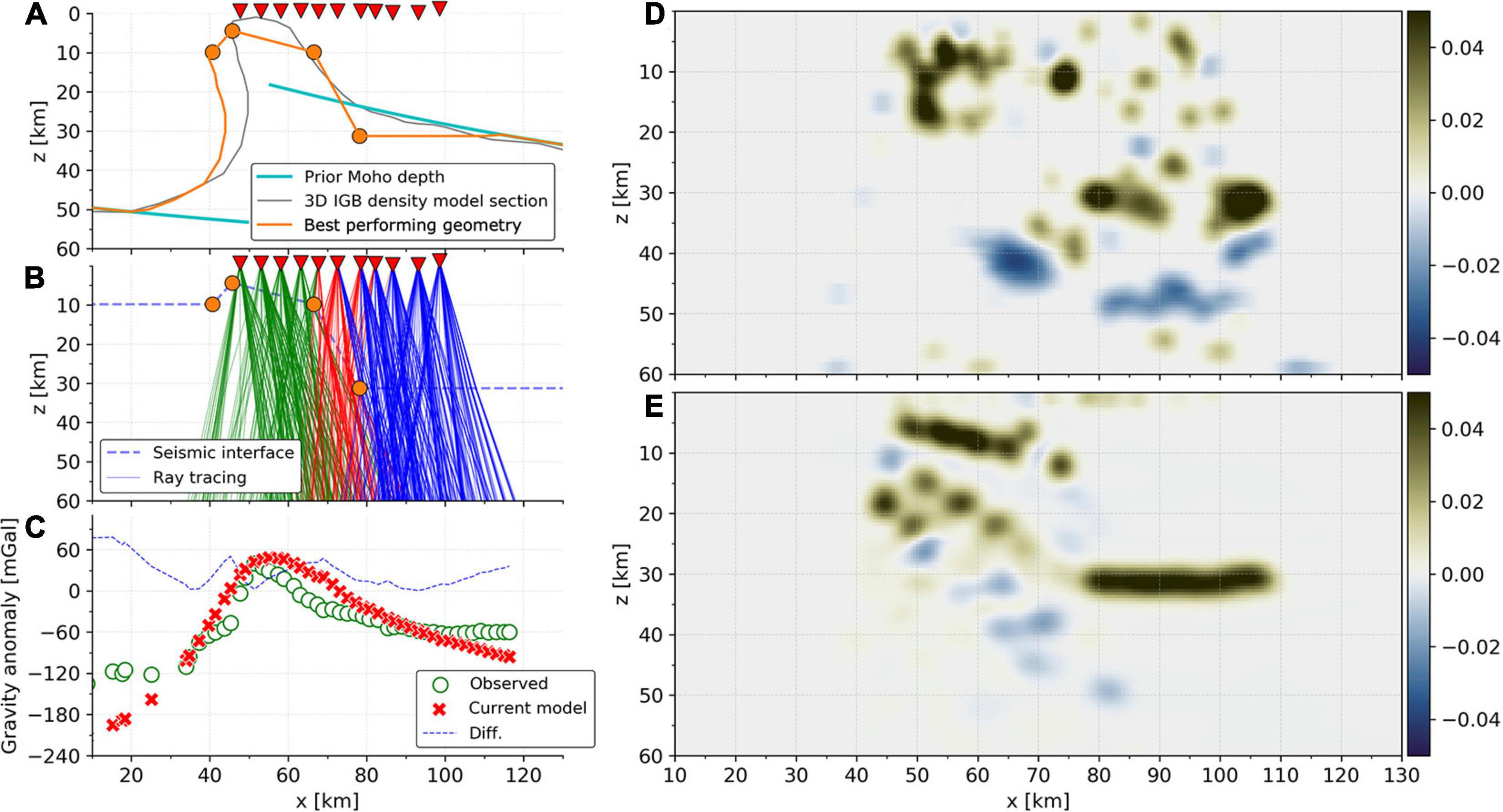
Figure 6. Example of forward model calculation demonstrated on the best performing IGB model. (A) The current model geometry (orange line), defined by four nodes (orange circles) and assumptions as in Figure 5. (B) Seismic ray-tracing across the model interface (blue dashed line segments) for the current velocity model. Seismic rays are colored according to the interface segment they cross along their path. The wave mode conversion respects Snell’s law considering the local interface dip. (C) Comparison between observed and synthetic gravity anomalies for the current model, and their misfit. (D) Observed-RFs migration, including ray-tracing and migration with the velocity structure of the current model. (E) Synthetic-RFs migration, using RFs generated by the current velocity structure, and then treated the same way as the observed RFs. The comparison between Observed-RFs and Synthetic-RFs migrations is obtained via image cross-correlation (further details in the text).
The solution of each seismic forward problem produces two new RF migration images, which we may refer to as the “synthetic” and the “observed” migration images, respectively.
The synthetic RF migration image is produced via three main steps: seismic ray-tracing, synthetic RFs computation and synthetic RFs migration (Figure 4, Seismic workflow).
Each of these steps always considers the candidate IGB model (or the current in the case of the first iteration): as a first step, we perform the ray-tracing across the candidate 2D velocity model structure for the same seismic catalog – station pairs, identical to the observed dataset. Snell’s law is respected at each model interface segment including local dip, meaning that it considers the relative angle between the propagating seismic trace and the dip (and depth) of the local interface segment (Figure 6B). The synthetic seismograms are computed via the Raysum software (Frederiksen and Bostock, 2000), whose code is wrapped in our inversion routine and receives as input the local IGB geometry along each ray-path.
Finally, the synthetic RFs are migrated along the candidate velocity structure with the computed ray-tracing, therefore producing the “synthetic” migration image. In addition, the observed RFs are migrated as well along the same candidate model and ray-tracing (Figures 6D,E), producing the so-called “observed” migration image. This allows to compare in a consistent manner the observed and the synthetic RFs for each given candidate model. The migrations pictures are spatially smoothed by 2D Gaussian ellipsoidal filter with 1.5 km and 0.75 km horizontal and vertical half-width. Noise, taken as low-amplitude signals at < 15 % of the image maximum amplitude, is removed from the observed migration picture. The final migration pictures have 0.5 km x 0.5 km pixel size.
We define the seismic model performance LS() as the zero-shift cross-correlation between the observed and synthetic RF migration images (Imobs and Imsyn):
where i is the pixel index and LS() is normalized, by definition, between -1 and 1.
For the gravity forward problem, we implemented direct formulas for the computation of gravity anomaly for a given density distribution. The distribution is defined as an n-sided polygon in a two-dimensional plane (Hubbert, 1948; Won and Bevis, 1987), under the assumption that the geometry extends unchanged toward infinity along the direction perpendicular to the profile (i.e., the out-of-plane coordinate). Therefore, we numerically treat the IGB model shape as a 2D polygon associated with a △ρ density contrast with respect to the surrounding background. The synthetic gravity anomaly is then computed for each of the binned gravity points (Figure 4, Gravity workflow).
Similarly, to the seismological part, we define the gravity misfit or model performance LG() as the zero-shift cross-correlation of the observed and synthetic gravity profiles Gobs and Gsyn:
where i is the single gravity point index and where LG() is normalized, by definition, between −1 and 1.
The problem of defining of a joint model performance (or joint misfit), combining the information from different geophysical data sets into the inversion process, has been addressed in the literature via different approaches. Various authors have introduced explicit scalar weighting parameters to accommodate for differences in the dataset’s noise and information content (e.g., Julia et al., 2000; Syracuse et al., 2016). Other authors have implicitly incorporated the weighting between different datasets in a more recent Bayesian formulation of their inverse problem (e.g., Bodin et al., 2012).
In our case, the objective functions are not set up on physical properties with values on different orders of magnitudes, but instead they are cross-correlation based. Therefore, in our case, we define our final model performance function as the direct multiplication between the seismic model performance and the gravity model performance, following a maximum likelihood principle (Drahos, 2008):
Thus, we obtain a performance measure for which we do not apply any user-defined weighting or scaling factor, and which, by definition, is normalized between −1 and 1.
Model Space Exploration
The model space exploration is carried out in a series of small random steps, with a new model being proposed at each of the iterations. Each of the model space coordinates mj (with j = 1,…,9) has been assigned with a pair of minimum and maximum values, mjmin and mjmax, within which the model coordinates can range during the inversion procedure (Table 1).
At each iteration, the exploration starts from the current model space location mcur (i.e., the initial or the latest accepted model sample) and randomly suggests a new candidate model mcand, related to mcur by:
where rj is a uniform random deviate and sj a scaling parameter.
We defined an acceptance rule to guide the acceptance or not of the newly proposed model mcand. Given L(mcand) the candidate model’s performance and L(mcur) the current model’s performance, mcand is accepted as model space sample if
where r is a random number between 0 and 1.
If mcand is accepted, it is updated as new current model and it becomes the starting point for the subsequent iteration; otherwise, the exploration stays at mcur and a new candidate model is proposed.
The acceptance rule we adopted follows the idea behind the Metropolis-Hastings algorithm, which is developed for sampling a probability density function defined over a model space (Sambridge and Mosegaard, 2002). We apply that idea and its acceptance rule here, in non-probabilistic terms, to guide our random walk toward better fitting areas of the model space. In fact, when providing a better fit to the data, the newly proposed model mcand is always accepted [i.e., when L(mcand) > L(mcur)]. The proposed model mcand can still be accepted, even when it provides a worse fit to the data compared to the current model mcur [i.e., when L(mcand) < L(mcur)]., as there still is a non-zero probability for the random number r – constrained between 0 and 1 – to be minor than L(mcand)/L(mcur): the lower the ratio, the lower the probability. The overall acceptance mainly depends on the shape of L(m) and on the distance between the current and the proposed model: △m = | mcand−mcur|. In fact, the algorithm requires a fine-tuning of the jump length, which is the only necessary user-defined parameter. Too little steps could cause the model space exploration to be trapped in a local minimum, without escaping and thus leaving wide regions of the model space unexplored. On the other hand, too long steps could provide model proposals too far away from the best fitting areas, causing too many rejections and waste of computational resources. For this reason and based on three preliminary tests we performed on subsets of the data, we rescale the uniform random deviates to be within the [0.05,0.25] interval, which provided a balanced compromise between model space exploration and exploitation.
The inversion on the full dataset was eventually run for 50’000 iterations. As we do not formulate the inverse problem in probabilistic terms, this prevents us from interpreting the sampled models as the realizations of a probability density function. Nevertheless, we used the a priori knowledge on the IGB to assign reasonable boundaries to all inversion parameters (as discussed in section “Model parameterization”) and we use a performance-driven pseudo-random walk to guide our exploration toward the best-fitting areas of the model space, to retrieve an ensemble of acceptable IGB models, which reproduce and explain the observed datasets.
Results
The inversion algorithm kept 41’363 models out of 50’000 iterations in one week of computation time on a standard computer (2.2GHz Quad-Core Intel Core i7), requiring ∼ 10s to 12s per iteration. Throughout the model space exploration, 20’692 steps were directed toward a better performing model and were therefore retained. The remaining sampled models were accepted based on Equation (6) even if they were not improving the performance with respect to the previous iteration, with an acceptance ratio of ∼ 70%. Exploration has been favored in spite of exploitation. By inspecting the distribution of all sampled models for all the model parameter pairs (Supplementary Material 3), a satisfactory model space coverage has been achieved for all the pairs. Less samples cover the worse fitting areas, while a higher sampling density concentrates around the best performing models.
The seismic model performances range from 0 to 0.64 with a nearly symmetric bell-shaped distribution and a median value of 0.26 (negative performances have been discarded by choice). The gravity model performances vary across a narrower range of values, between 0.59 and 0.99, with a negative skew (more frequent higher values) and a median of 0.90 (Supplementary Material 4). The better performance of the model with respect to gravity data is not surprising, as our a priori choices for the model geometry were driven by the recently constrained 3D gravity model. Therefore, in the final model performance, defined as the multiplication of seismic and gravity fits, the seismic performance acted as a more important guiding factor for the model space exploration. The gravity performance provided finer tuning across the best fitting areas, and also resolved some of the inherent trade-off in RF analysis. Furthermore, jointly inverting with seismic data allowed to constrain geometry features which were not resolvable with a gravity-only inversion, as demonstrated by preliminary tests (Supplementary Material 6). The final model performances range between 0 and 0.60, with a median value of 0.22.
The results reproduce well the main features of the observed seismic and gravity anomalies.
First, we describe the best performing model and then we consider the group of 150 best fitting models.
The best performing model fits the gravity anomalies both in terms of location and amplitude, with a slightly broader peak compared to the observations (Figure 6C). The vertical part of the IGB model is wider than what was suggested by the earlier, 3D gravity model (Scarponi et al., 2020). Node 2 locates the shallowest IGB portion in the vicinity of the western kink of the previous model (Figure 6A), as shallow as 4 km depth, and West of seismological station IA01A and of the IL at the surface. This location is a few kilometers too far to the West considering the local a priori geological knowledge. Concerning the migration images, the shallowest interface segment (node 2 to node 3) successfully reproduces the shallowest converted phases in the western portion of the profile, locating a sharp increase of shear-wave velocity right below the surface, between 3 and 7 km depth, and extending for ∼ 20 km to the East from station IA01A to station IA05A (Figures 6D,E). Minor local features are recovered as well, such as the positive patch at ∼ 75 km distance and at 12 km depth, and further reverberations at ∼ 45 km distance and 15 km depth, below the shallowest conversion. The eastern portion of the image with prominent signals at ∼ 35 km depth is recovered and consistent with the Moho depth further to the East (Figures 6A,D,E).
Using a single interface model prevents us from reproducing the eastern negative amplitudes at ∼ 48 km depth ranging from 80 to 105 km distance, which cannot be regarded a converted-phase multiple reflection (PpSs) from an interface at 34 km depth. Such phase would be expected at a higher delay time (∼ 19 s with the given model structure and therefore migrated at more than 100 km depth). This feature can represent a real decrease of shear-wave seismic velocity with depth, or PpSs multiples of local conversions seen in the upper crust (Figure 6D) which are not modeled in this distance range.
A more representative image of the joint inversion results is provided by looking at the ensemble of the 150 best performing models (Figure 7). From this, the general characteristics of the retrieved well-fitting IGB model geometries can be outlined. It still is a shallow-reaching, crustal-scale important geophysical anomaly, similar to our earlier 3D gravity model (Scarponi et al., 2020), but without a prominent westward extending horizontal “beak” as in the historical model of Berckhemer (1968),. A shallow interface is always present in the western part of the profile between 1 and 10 km depth, between IA01A and IA05A stations (∼40 to 70 km distance). The position of the vertical structures is less constrained than the horizontal ones, as the steeply dipping structures cannot be imaged by the RFs at all. The shape of the western IGB vertical wall was inherited by the previous 3D gravity model (Scarponi et al., 2020) and its horizontal position was here varied together with node 1. The range of variation of either side of the IGB neck spans ∼ 15 km horizontally, while the horizontal segments span a narrower depth range (less than 10 km). In the western part, the neck is on average 30 ± 5 km wide, only a few models deviate up to ± 10 km width. The main IGB discontinuity is tightly constrained in the eastern, flat part of the profile at 35 km depth (Figure 7), which is consistent with the Moho structure there (Spada et al., 2013).
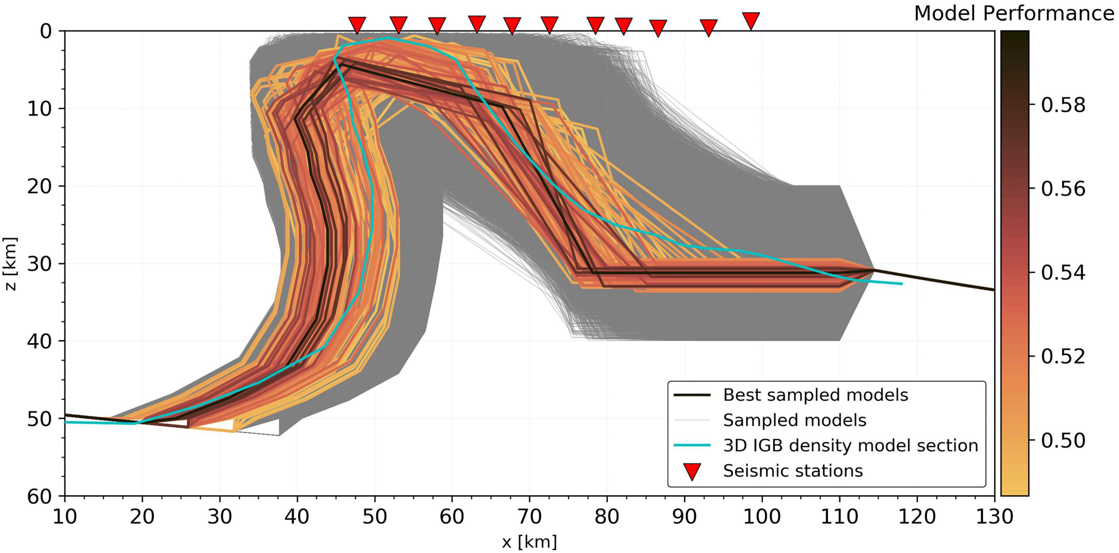
Figure 7. Model geometries resulting from the joint inversion. The 150 best performing models are shown in colored lines according to the model performance. All other sampled and kept models are shown in gray (in total 41’365 models). The cyan dashed line is the cross-section through the 3D IGB gravity model from previous study (Scarponi et al., 2020).
How well the IGB-top interface geometry is constrained by the joint inversion can be assessed through the distribution of the sampled model nodes position, which also shows the characteristics of the model space exploration (Figure 8). All four nodes have spanned the entire allowed perimeter, with a decreasing sampling density toward the worse-fitting external boundaries, and with node 2 being more restricted by definition of its position lying between and above nodes 1 and 3 (Figure 8). This proves the efficiency of the implemented algorithm in providing a satisfactory model space exploration, which is computationally much more affordable than a 9-dimensional full grid search at a comparable resolution. In general, node depths are better constrained better than their horizontal locations. The depth-variation range of ∼ 10 km for node 1 to ∼ 4-5 km for node 4.
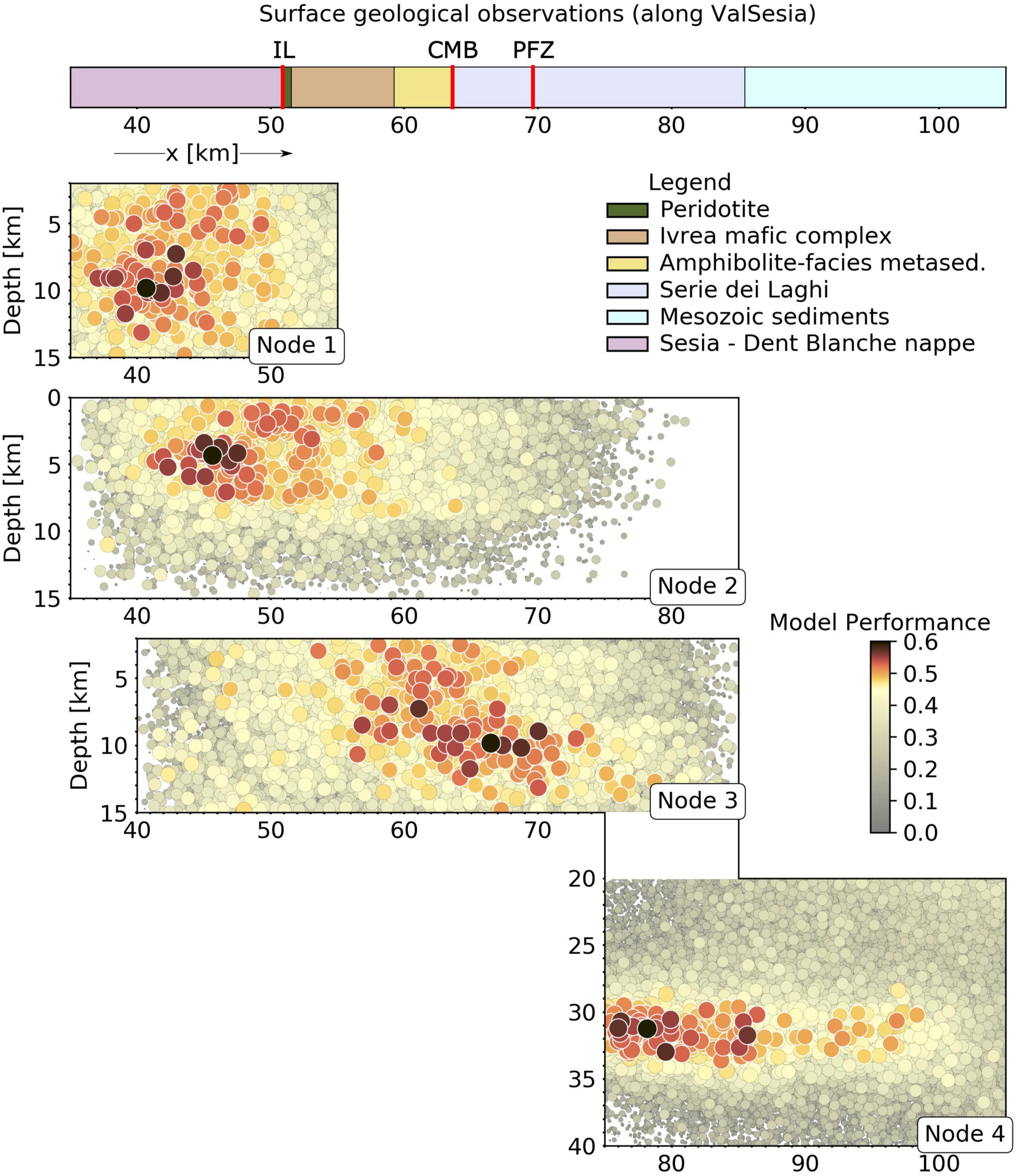
Figure 8. Inversion results on the position of the four nodes, presented in four distance–depth panels. Each panel is showing the locations visited by each single node during the inversion, for each sampled model. All four panels share the same horizontal X-axis, but they are shifted along the vertical direction for better visual distinction. Panels of nodes 3 and 4 share the same depth axis, too. All sampled and kept models are shown (in total 41’363), with size and color according to the model performance, plus all models with performance higher than 0.48 are indicated by white edges. Each panel is limited to the allowed range of parameter values. On top, the corresponding surface geological observations from earlier studies (along the same X-axis), identifying rock types along the profile (legend on the top right, same as in Figure 2). The relevant faults for this study are indicated (as in Figure 2) as “IL” for Insubric Line, “CMB” for Cossato-Mergozzo-Brissago Line and “PFZ” for Pogallo Fault Zone.
Node 1 solutions are preferentially at 10 km depth to West of the IL, which is in agreement with the IL being a vertical to sub-vertical dipping feature. Node 2 constrains the shallowest model position and features a bi-modal depth result, with a group of solutions between ∼ 1-3 km at x = 50-55 km. This finding is in agreement with the outcropping dense rocks at the surface. Another group of solutions concentrate at ∼ 3-7 km depth to the West of the surface trace of the IL. Node 3 isn’t tightly constrained; nevertheless, it extends the shallow IGB portion to the center of the seismic profile, until the surface trace of the Pogallo Fault Zone (PFZ), prior to high-angle deepening toward node 4 at 31 ± 2 km depth (Figure 8).
Concerning the physical property contrasts of the IGB compared to the shallower layer (Figure 9), the well-performing models point to a relatively broad range of shear-wave seismic velocity increases. This is mainly constrained by the amplitude of the Ps signals, which is not their most reliable feature due to attenuation. A certain number of better-performing models is associated with a velocity contrast of the order of 0.5 to 1.2 km/s. The best performing density contrasts are in the 200 to 400 kg/m3 range, with some models at 500 kg/m3 associated to the higher vS contrasts. This is in good agreement with the earlier 3D gravity model which suggested that 500 kg/m3 represents a reasonable higher limit for the IGB density contrast (e.g., Scarponi et al., 2020). We note that models with very high density- and low velocity-contrasts perform poorly (Figure 9).
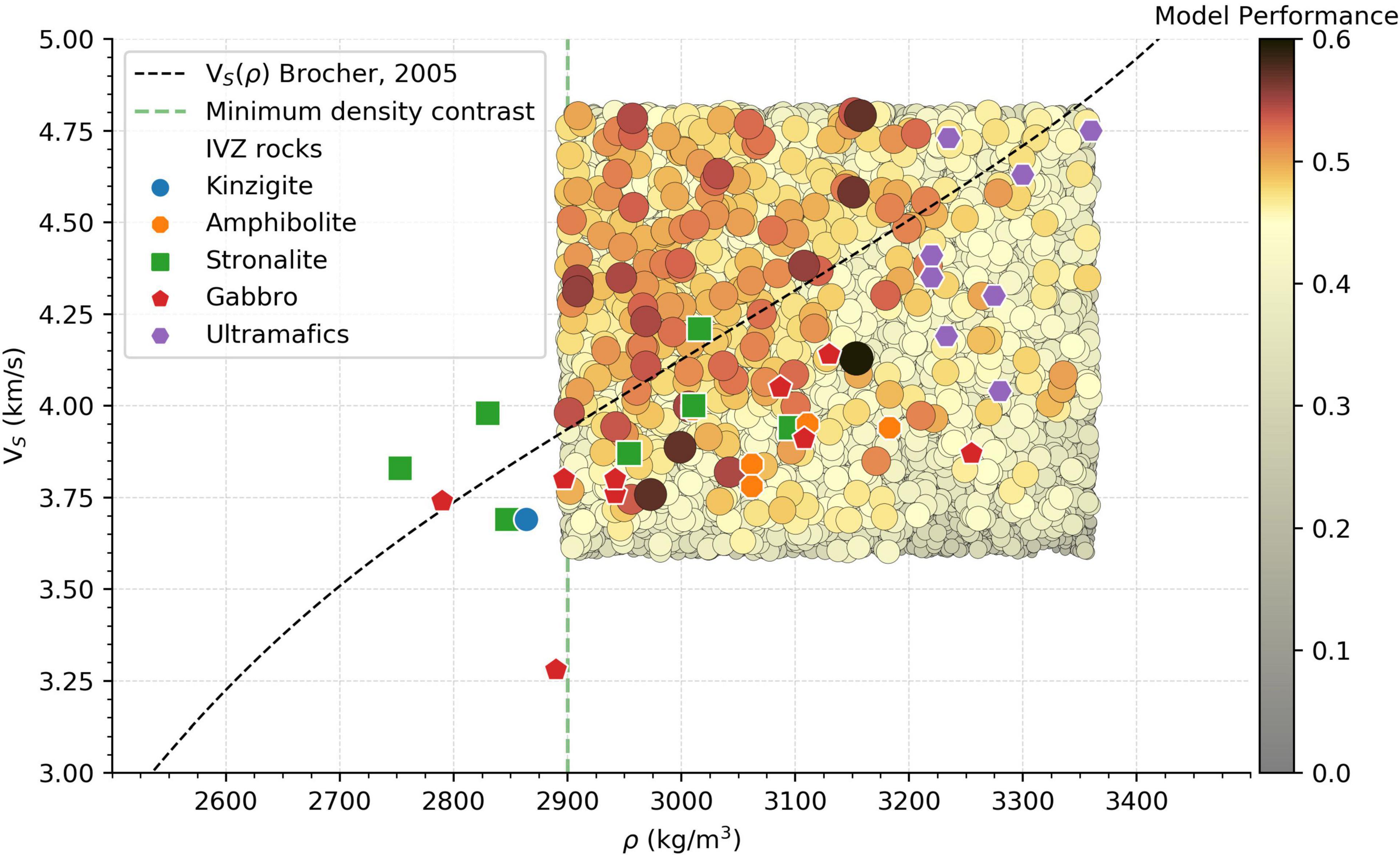
Figure 9. Inversion results on the density and shear-wave velocity contrasts associated with the 2D model interface, shown as gray-contoured circles of size and color according to to the model performance. The background density and the background shear-wave velocity absolute values are common for all models (2700 kg/m3 and 3.5 km/s, respectively). For comparison, the regression fit for the vs(ρ) relationship from rocks discussed in Brocher (2005) (black dashed line) is shown together with a relevant set of rock physical properties across the IVZ from the SAPHYR catalog (Zappone et al., 2015).
We note that the gravimetric method is able to resolve density contrasts, and not absolute densities. Therefore, the set of inversion results on Figure 9 can be shifted to the right, to higher density values, by simply assuming that the surrounding crustal density was not 2700 kg/m3 but higher. A geologically reasonable shift would be around 100 kg/m3: a density of 2800 kg/m3 is reasonable for mid-crustal rocks; hence, the well-fitting models from the joint inversion would fall closer to the vS–ρ relationship trend taken from Brocher (2005). We note that the trend line of Brocher (2005) represents empirical fits, and that actual rock property data dispersions of 0.2 km/s in vS or of 200 kg/m3 are reasonable.
Discussion
The inversion results can be interpreted in light of the existing multidisciplinary investigations on the IVZ formation history and the surrounding crustal structures. By inspecting the best performing IGB models (Figure 7), two main groups of models can be identified according to the shallow geometry characteristics of the retrieved IGB models (Figures 7, 8, node 2). The first group of models suggests a gently eastward-dipping interface in the shallow portion, locating the IGB-top head from ∼ 3–7 km depth (node 2) to ∼ 8–12 km depth (node 3) with a minimum horizontal extent of ∼ 20 km. The second group of models features node 2 at clearly shallower depths than nodes 1 and 3, reaching as shallow as 1-3 km depth between seismological stations IA01A and IA03A. While both groups are in agreement with a western boundary associated with a steeply westward dipping IL, the very shallow anomaly of the latter group agrees with the well-known variety of lower to middle crustal rock outcrops observed across the IVZ. Moreover, when compared with the rock properties of in situ IVZ samples (Zappone et al., 2015) in vS–ρ space, the inversion results show good agreement with several gabbro samples, and also with ultramafic rock and amphibolite samples if the aforementioned density-shift is considered (Figure 9). These align with indications drawn from studies by Pistone et al. (2020) and Scarponi et al. (2020) on possible rock types. However, we make no further selection of rock types, to avoid potential over-interpretation here, as reality is surely more complex than a single-discontinuity 2D model. Nevertheless, considering the model assumptions, the match with rock properties is satisfactory.
An interesting feature of sampled IGB model structures is the steep eastward-dipping segment at the center of our profile between nodes 3 and 4 (∼ 70-75 km distance, Figure 7), representing the eastern flank of the IGB. The steepness of this segment precludes any direct imaging by the RFs. The segment, however, joins the two surrounding and imaged segments (between nodes 2 and 3 and east of node 4) and it compares well with the location at the surface of the Pogallo Fault Zone (PFZ, Figure 8). The PFZ is a prominent Jurassic fault zone associated with pre-orogenic crustal thinning episodes, related to the opening of the Alpine Tethys without being subsequently reactivated during the orogenic compression, but only tilted to its present-day vertical position (Handy et al., 1999; Petri et al., 2019).
The PFZ crosses our seismic profile at the surface at the Lago d’Orta, between stations IA05A and IA06A. Several evidences suggest that the PFZ may have offset the Moho during the Jurassic (Handy, 1987) and that the shape of the IGB was determined by a combination of Jurassic crustal thinning and subsequent Alpine orogeny (Schmid et al., 1987). The importance of pre-orogenic inheritance with respect to syn-orogenic processes is however, clearer in the light of our results. Along our profile, the eastern flank of the IGB coincides much more closely with the surface exposure of the PFZ than what was pointed at by previous models (Berckhemer, 1968): the PFZ is likely responsible for shaping the Moho since the Jurassic, implying that the IGB was strongly pre-set by the pre-orogenic rift-related deformations, before being integrated in the Alpine orogeny.
In light of the planned scientific drilling in Val Sesia (Pistone et al., 2017), we further investigated one particular property of the shallowest portion of the IGB interface, namely the sharpness of the velocity discontinuity, by applying frequency-dependent RF analysis. In fact, the frequency content of the observed RFs can put constraints on the resolved thickness of the seismic velocity gradient associated with the converted-wave generating interface itself (James et al., 2003). The narrower the peaks with increasing RF analysis frequency, the sharper the interface at which the conversion was produced. Conversely, if there is a vertical gradient, the highest frequency RFs will remain broad and lose amplitude. We demonstrate this effect by synthetics, which we then compared with the observed RFs. We focused our analysis on station IA02A and stacked a high-quality selection of RFs, for a certain number of high-pass filtering frequencies: 1, 2, 3, 4, and 6 Hz, respectively (Figure 10A). We used RFs in the ZRT coordinate system and only for eastward [45-135°] back-azimuths to maximize the Ps conversion amplitude on the inferred eastward dipping interface. The RF stacks show two shallow conversion peaks at ∼ 3 and 6 km depth (Figure 10A). Considering the respective piercing points, the two peaks correspond to early arrivals from ENE to late arrivals from ESE. This points to local structural variations at shallow depth beneath the gabbro and norite rocks exposed on the surface (Figure 10B). Comparing our results to the synthetics shown in Figures 10C–E) indicates that the velocity gradient thickness is more than 0.4 km, and closer to but less than 0.8 km. This is slightly more than the Moho transition zone of 0.5 km proposed for the Kaapvaal craton by James et al. (2003), based on a similar seismic analysis. Our finding is well-resolved as the wavelength of 6 Hz waves at vS of 3.5 km/s is below 600 m, so this approach would have been able to resolve sharper gradients.
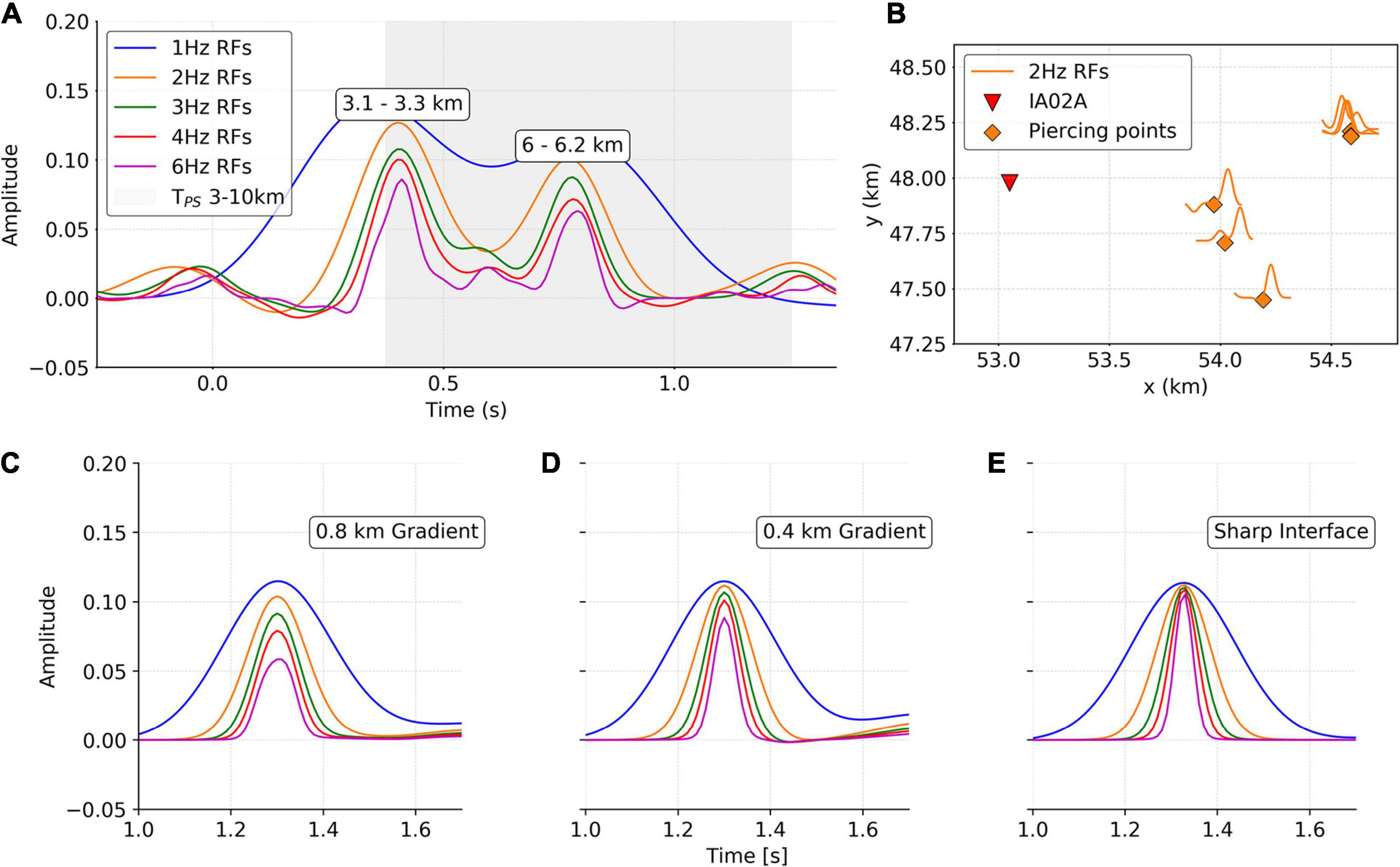
Figure 10. Investigating the sharpness of the seismic interface by frequency-dependent analysis of the highest quality RFs near station IA02A. (A) Observed RFs stacked at different frequency ranges, from 0.1 Hz to five different maximum frequencies as specified in the legend. The decreasing signal width, with increasing frequency, points toward a discontinuity sharper than the resolution of the highest frequency waves. The gray band in the background indicates the expected time delay for a P-to-S converted phase from a discountinuity located between 3 and 10 km depth, and with vs = 3.5 km/s above it. The estimated depth of the conversion for the two observed peaks is indicated. For this analysis, a stricter quality control has been applied and only the RFs qualifying at all frequency ranges have been considered. (B) Piercing point map (orange squares) for the traces that have been considered in (A), for the frequency range 0.1 Hz to 2 Hz. Next to each piercing point, the time interval 0 to 1s of the associated RFs is plotted, to highlight the spatial variability of the stacked RFs signals. (C–E) Synthetic RFs for the same frequencies as in (A) demonstrating the effect of velocity gradient sharpness on peak widths and amplitudes.
Future contributions could address the IGB structure by inverting for more complicated geometries, including more than one seismic interface. P-to-SH converted phases could be addressed as well, as they do present seismic energy due to the presence of dipping angles and possibly anisotropy, which was not addressed in this contribution as there were strong a priori indications for dip. Much finer, high-resolution images of the western part of our area will be revealed with the recently acquired active seismic data with Vibroseis sources and several targets at depth along two long profiles crossing between stations 1 and 2, and carried out as a cooperative project between GFZ Potsdam, Montanuniversität Leoben and the University of Lausanne. We plan to complement these with higher resolution gravimetric and magnetic measurements around the Balmuccia peridotite, to approach the scale of scientific drilling. Subsequent, joint petrological and geophysical investigations will further constrain the lithologies composing the IGB.
Conclusion
We implemented and ran a joint inversion algorithm using seismic receiver functions and gravity data to constrain the shape and the physical properties of the Ivrea Geophysical Body (IGB), along a 2D West-East cross-section along the Val Sesia profile and across the Ivrea-Verbano Zone (IVZ). The algorithm executes a performance-driven random walk in the model space, to preferentially explore the better fitting areas of the model space.
Processing the new seismological and recently collected gravity data led to new constraints on the IGB structure. A shallow and relatively sharp interface is resolved over at least 20 km horizontal distance in the western part of the seismic profile (between ∼ 8.11°E and 8.43°E). In particular, we identify two main groups of model geometries for the shallowest portion of the IGB: a flat and gently eastward-dipping interface between 3 and 7 km depth, and a structure with a local peak reaching as shallow as 1-3 km depth, beneath the three westernmost stations (∼ 8.11°E to 8.25°E). While both groups of models agree with a western boundary associated with the steeply westward-dipping Insubric Line, the latter is more consistent with the well-known lower crustal rock complex outcropping at the western edge of the IVZ. Further agreement with the observed geological structures at the surface is found by comparing the IGB model structure with the location of the Pogallo Fault Zone (PFZ). The eastern flank of the protruding IGB coincides with the surface exposure of the Jurassic PFZ, highlighting the role of pre-orogenic processes in shaping the IGB.
The retrieved IGB velocity and density contrasts relative to the surroundings are in general good agreement with the physical properties of the rock samples collected in the area and analyzed in earlier studies. The results span a rather broad range of acceptable shear-wave velocity contrasts (0.5 to 1.2 km/s), providing slightly higher velocities than those from field samples and/or trends in the literature (Brocher, 2005). In terms of density, a reasonably narrow range of better-fitting density contrasts of 200–400 kg/m3 is found, in agreement or slightly below the recent 3D IGB density model.
We further analyzed the amplitude and frequency content of a stack of selected high-quality receiver functions, to constrain the sharpness of the vertical velocity-gradient associated with the shallow IGB discontinuity. We then compared the observed stack with synthetics, for a range of different pre-deconvolution maximum filtering frequencies, and using various vertical velocity-gradient thicknesses. We found thicknesses of 0.8 km and 0.4 km as reasonable higher and lower limits for the shallow velocity-gradient mimicking the top of the IGB discontinuity. Already acquired but still in-the-processing active seismic campaign data will shed more light on the very shallow structure at high resolution along the same profile, and prepare the ground for deep scientific drilling to deepen our knowledge of the IGB.
Data Availability Statement
The new seismic data will be openly and freely available from September 2022 through the ORFEUS data center, under the FDSN network code XK and is already referenced at the following doi: 10.5281/zenodo.1038209. The gravity dataset is available upon request to either of the first two authors.
Author Contributions
MS and GH designed the study. MS, GH, JP, SS, and LB collected the new field data. MS performed the processing and inversion with guidance from GH. MS and GH drafted the manuscript. MS, GH, JP, SS, and BP discussed the obtained results. All authors revised the manuscript and approved the final version.
Funding
We acknowledge the Swiss National Science Foundation (SNF) for having supported this research (grant numbers PP00P2_157627 and PP00P2_187199 of project OROG3NY), as well as the Grant Agency of the Czech Republic (No. 21-25710). We also acknowledge project CzechGeo/EPOS No. LM2015079 of the MEYS for funding the MOBNET station pool.
Conflict of Interest
The authors declare that the research was conducted in the absence of any commercial or financial relationships that could be construed as a potential conflict of interest.
Acknowledgments
We would like to acknowledge many colleagues for their precious contributions and various inputs that made this work possible, both in the field and during the subsequent steps to P. Jedlièka, J. Kotek, and L. Vecsey from Institute of Geophysics, Czech Academy of Sciences, for installation of seismic stations within this project (stations of MOBNET pool, granted by project CzechGeo/EPOS No. LM2015079 of the MEYS) and for seismic data pre-processing, formatting, and checking; T. Berthet, L. Colavitti, S. Subedi, G. Moradi, C. Alvizuri, and the whole IvreaArray working team for the discussions and fieldwork efforts, together with numerous people in the field area for their help and support during the measurement campaigns, and the seismic sensors installation and maintenance: in particular to the mayors and the local contacts in the communes of Boccioleto, Vocca-Sassiglioni, Varallo, Civiasco, Cesara, Cheggino, Nebbiuno, Calogna, Ispra, and Biandronno; U. Marti, R. Barzaghi, the OGS institution, A. Zappone, T. Diehl, R. Cattin, and S. Mazzotti for sharing background data, internal discussions, and the GravProcess software sharing and editing. We are grateful for the enthusiastic support of many colleagues from the DIVE project, especially Othmar Müntener, Alberto Zanetti, Mattia Pistone, Andrew Greenwod, Luca Ziberna, and Klaus Holliger.
Supplementary Material
The Supplementary Material for this article can be found online at: https://www.frontiersin.org/articles/10.3389/feart.2021.671412/full#supplementary-material
Footnotes
References
Ammon, C. J., Randall, G. E., and Zandt, G. (1990). On the nonuniqueness of receiver function inversions. Journal of Geophysical Research: Solid Earth 95, 15303–15318.
Ansorge, J. (1979). Crustal section across the zone of Ivrea-Verbano from the Valais to the Lago Maggiore. Bollettino di Geofisica Teorica ed Applicata 21, 149–157.
Basuyau, C., and Tiberi, C. (2011). Imaging lithospheric interfaces and 3D structures using receiver functions, gravity, and tomography in a common inversion scheme. Computers & geosciences 37, 1381–1390.
Bayer, R., Carozzo, M., Lanza, R., Miletto, M., and Rey, D. (1989). Gravity modelling along the ECORS-CROP vertical seismic reflection profile through the Western Alps. Tectonophysics 162, 203–218.
Berckhemer, H. (1968). Topographie des “Ivrea-Körpers” abgeleitet aus seismischen und gravimetrischen Daten: Schweiz. Mineral. Petrogr. Mitt 48, 235–246.
Berger, A., Mercolli, I., Kapferer, N., and Fügenschuh, B. (2012). Single and double exhumation of fault blocks in the internal Sesia-Lanzo Zone and the Ivrea-Verbano Zone (Biella, Italy). International Journal of Earth Sciences 101, 1877–1894.
Bodin, T., Sambridge, M., Tkalèiæ, H., Arroucau, P., Gallagher, K., and Rawlinson, N. (2012). Transdimensional inversion of receiver functions and surface wave dispersion. Journal of Geophysical Research: Solid Earth 117, B02301.
Brack, P., Ulmer, P., and Schmid, S. M. (2010). A crustal-scale magmatic system from the Earth’s mantle to the Permian surface: Field trip to the area of lower Valsesia and Val d’Ossola (Massiccio dei Laghi, Southern Alps, Northern Italy). Swiss Bulletin für angewandte Geologie 15, 3–21.
Brocher, T. M. (2005). Empirical relations between elastic wavespeeds and density in the Earth’s crust. Bulletin of the seismological Society of America 95, 2081–2092.
Bürki, B. (1990). “Geophysical interpretation of astrogravimetric data in the Ivrea Zone,” in Exposed Cross-Sections of the Continental Crust, eds M. H. Salisbury and D. M. Fountain (Dordrecht: Springer), 545–561.
Cattin, R., Mazzotti, S., and Baratin, L.-M. (2015). GravProcess: An easy-to-use MATLAB software to process campaign gravity data and evaluate the associated uncertainties. Computers & geosciences 81, 20–27.
De Franco, R., Biella, G., Boniolo, G., Corsi, A., Demartin, M., Maistrello, M., et al. (1997). Ivrea seismic array: a study of continental crust and upper mantle. Geophysical Journal International 128, 723–736.
Diehl, T., Husen, S., Kissling, E., and Deichmann, N. (2009). High-resolution 3-DP-wave model of the Alpine crust. Geophysical Journal International 179, 1133–1147.
Drahos, D. (2008). Determining the objective function for geophysical joint inversion. Geophysical Transactions 45, 105–121.
Fountain, D. M. (1976). The Ivrea—Verbano and Strona-Ceneri Zones, Northern Italy: a cross-section of the continental crust—new evidence from seismic velocities of rock samples. Tectonophysics 33, 145–165.
Frederiksen, A., and Bostock, M. (2000). Modelling teleseismic waves in dipping anisotropic structures. Geophysical Journal International 141, 401–412.
Handy, M., Franz, L., Heller, F., Janott, B., and Zurbriggen, R. (1999). Multistage accretion and exhumation of the continental crust (Ivrea crustal section, Italy and Switzerland). Tectonics 18, 1154–1177.
Handy, M. R. (1987). The structure, age and kinematics of the Pogallo Fault Zone; Southern Alps, northwestern Italy. Eclogae Geologicae Helvetiae 80, 593–632.
Handy, M. R., Schmid, S. M., Bousquet, R., Kissling, E., and Bernoulli, D. (2010). Reconciling plate-tectonic reconstructions of Alpine Tethys with the geological–geophysical record of spreading and subduction in the Alps. Earth-Science Reviews 102, 121–158.
Handy, M. R., Ustaszewski, K., and Kissling, E. (2015). Reconstructing the Alps–Carpathians–Dinarides as a key to understanding switches in subduction polarity, slab gaps and surface motion. International Journal of Earth Sciences 104, 1–26.
Hetényi, G., Plomerová, J., Bianchi, I., Exnerová, H. K., Bokelmann, G., Handy, M. R., et al. (2018). From mountain summits to roots: Crustal structure of the Eastern Alps and Bohemian Massif along longitude 13.3 E. Tectonophysics 744, 239–255.
Hetényi, G., Plomerová, J., Solarino, S., Scarponi, M., Vecsey, L., Munzarová, H., et al. (2017). IvreaArray—an AlpArray complementary experiment. doi: 10.5281/zenodo.1038209
Hetényi, G., Ren, Y., Dando, B., Stuart, G. W., Hegedûs, E., Kovács, A. C., et al. (2015). Crustal structure of the Pannonian basin: the AlCaPa and Tisza Terrains and the Mid-Hungarian zone. Tectonophysics 646, 106–116.
Hubbert, M. K. (1948). A line-integral method of computing the gravimetric effects of two-dimensional masses. Geophysics 13, 215–225.
James, D. E., Niu, F., and Rokosky, J. (2003). Crustal structure of the Kaapvaal craton and its significance for early crustal evolution. Lithos 71, 413–429.
Julia, J., Ammon, C., Herrmann, R., and Correig, A. M. (2000). Joint inversion of receiver function and surface wave dispersion observations. Geophysical Journal International 143, 99–112.
Kennett, B., and Engdahl, E. (1991). Traveltimes for global earthquake location and phase identification. Geophysical Journal International 105, 429–465.
Khazanehdari, J., Rutter, E., and Brodie, K. (2000). High−pressure−high−temperature seismic velocity structure of the midcrustal and lower crustal rocks of the Ivrea−Verbano zone and Serie dei Laghi, NW Italy. Journal of Geophysical Research: Solid Earth 105, 13843–13858.
Kissling, E. (1993). Deep structure of the Alps—what do we really know? Physics of the Earth and Planetary Interiors 79, 87–112.
Kissling, E., Wagner, J., and Mueller, S. (1984). “Three-dimensional gravity model of the northern Ivrea-Verbano Zone,” in Geomagnetic and Gravimetric Studies of the Ivrea Zone: Matér. Géol. Suisse. Géophys, Vol. 21, eds J.-J. Wagner and St Müller 55–61.
Langston, C. A. (1979). Structure under Mount Rainier, Washington, inferred from teleseismic body waves: Journal of Geophysical Research. Solid Earth 84, 4749–4762.
Lanza, R. (1982). Models for interpretation of the magnetic anomaly of the Ivrea body. Geologie Alpine 58, 85–94.
Levin, V., and Park, J. (1997). Crustal anisotropy in the Ural Mountains foredeep from teleseismic receiver functions. Geophysical Research Letters 24, 1283–1286.
Ligorría, J. P., and Ammon, C. J. (1999). Iterative deconvolution and receiver-function estimation. Bulletin of the seismological Society of America 89, 1395–1400.
Masson, F., Verdun, J., Bayer, R., and Debeglia, N. (1999). Une nouvelle carte gravimétrique des Alpes occidentales et ses conséquences structurales et tectoniques. Comptes Rendus de l’Académie des Sciences-Series IIA-Earth and Planetary Science 329, 865–871.
Moorkamp, M., Jones, A., and Fishwick, S. (2010). Joint inversion of receiver functions, surface wave dispersion, and magnetotelluric data. Journal of Geophysical Research: Solid Earth 115, B04318.
Nicolas, A., Hirn, A., Nicolich, R., and Polino, R. (1990). Lithospheric wedging in the western Alps inferred from the ECORS-CROP traverse. Geology 18, 587–590.
Niggli, E. (1946). Über den Zusammenhang zwischen der positiven Schwereanomalie am Südfuß der Westalpen und der Gesteinszone von Ivrea. Eclogae Geologicae Helvetiae 39, 211–220.
Petri, B., Duretz, T., Mohn, G., Schmalholz, S. M., Karner, G. D., and Müntener, O. (2019). Thinning mechanisms of heterogeneous continental lithosphere. Earth and Planetary Science Letters 512, 147–162.
Pistone, M., Müntener, O., Ziberna, L., Hetényi, G., and Zanetti, A. (2017). Report on the ICDP workshop DIVE (Drilling the Ivrea–Verbano zonE). Scientific Drilling 23, 47–56.
Pistone, M., Ziberna, L., Hetényi, G., Scarponi, M., Zanetti, A., and Müntener, O. (2020). Joint Geophysical−Petrological Modeling on the Ivrea Geophysical Body Beneath Valsesia, Italy: Constraints on the Continental Lower Crust. Geochemistry, Geophysics, Geosystems 21, e2020GC009397.
Rey, D., Quarta, T., Mouge, P., Miletto, M., and Lanza, R. (1990). Gravity and aeromagnetic maps of the western Alps: contribution to the knowledge of the deep structures along the ECORS-CROP seismic profile. Mémoires de la Société géologique de France (1833) 156, 107–121.
Sambridge, M. (1999). Geophysical inversion with a neighbourhood algorithm—I. Searching a parameter space. Geophysical journal international 138, 479–494.
Sambridge, M., and Mosegaard, K. (2002). Monte Carlo methods in geophysical inverse problems. Reviews of Geophysics 40, 3–1.
Scarponi, M., Hetényi, G., Berthet, T., Baron, L., Manzotti, P., Petri, B., et al. (2020). New gravity data and 3-D density model constraints on the Ivrea Geophysical Body (Western Alps). Geophysical Journal International 222, 1977–1991.
Schmid, S., Aebli, H., Heller, F., and Zingg, A. (1989). The role of the Periadriatic Line in the tectonic evolution of the Alps. Geological Society, London, Special Publications 45, 153–171.
Schmid, S. M., Kissling, E., Diehl, T., van Hinsbergen, D. J., and Molli, G. (2017). Ivrea mantle wedge, arc of the western alps, and kinematic evolution of the alps-apennines orogenic system. Swiss J. Geosci. 110, 581–612. doi: https://doi.org/10.1007/s00015-016-0237-0
Schmid, S., and Kissling, E. (2000). The arc of the western Alps in the light of geophysical data on deep crustal structure. Tectonics 19, 62–85.
Schmid, S., Zingg, A., and Handy, M. (1987). The kinematics of movements along the Insubric Line and the emplacement of the Ivrea Zone. Tectonophysics 135, 47–66.
Schmid, S. M., Fügenschuh, B., Kissling, E., and Schuster, R. (2004). Tectonic map and overall architecture of the Alpine orogen. Eclogae Geologicae Helvetiae 97, 93–117.
Shibutani, T., Sambridge, M., and Kennett, B. (1996). Genetic algorithm inversion for receiver functions with application to crust and uppermost mantle structure beneath eastern Australia. Geophysical Research Letters 23, 1829–1832.
Solarino, S., Malusà, M. G., Eva, E., Guillot, S., Paul, A., Schwartz, S., et al. (2018). Mantle wedge exhumation beneath the Dora-Maira (U) HP dome unravelled by local earthquake tomography (Western Alps). Lithos 296, 623–636.
Spada, M., Bianchi, I., Kissling, E., Agostinetti, N. P., and Wiemer, S. (2013). Combining controlled-source seismology and receiver function information to derive 3-D Moho topography for Italy. Geophysical Journal International 194, 1050–1068.
Subedi, S., Hetényi, G., Vergne, J., Bollinger, L., Lyon-Caen, H., Farra, V., et al. (2018). Imaging the Moho and the Main Himalayan Thrust in Western Nepal with receiver functions. Geophysical Research Letters 45, 13222–13230.
Syracuse, E. M., Maceira, M., Prieto, G. A., Zhang, H., and Ammon, C. J. (2016). Multiple plates subducting beneath Colombia, as illuminated by seismicity and velocity from the joint inversion of seismic and gravity data. Earth and Planetary Science Letters 444, 139–149.
Thouvenot, F., Paul, A., Senechal, G., Hirn, A., and Nicolich, R. (1990). ECORS-CROP wide-angle reflection seismics: constraints on deep interfaces beneath the Alps: Mém. Soc. Géol. France 156, 97–106.
Vecchia, O. (1968). La zone Cuneo-Ivrea-Locarno, élément fondamental des Alpes. Géophysique et géologie: Schweizerische Mineralogische Petrographische Mitteilungen 48, 215–226.
Vinnik, L. P., Reigber, C., Aleshin, I. M., Kosarev, G. L., Kaban, M. K., Oreshin, S. I., et al. (2004). Receiver function tomography of the central Tien Shan. Earth and Planetary Science Letters 225, 131–146.
Won, I., and Bevis, M. (1987). Computing the gravitational and magnetic anomalies due to a polygon: Algorithms and Fortran subroutines. Geophysics 52, 232–238.
Zappone, A., Wenning, Q. C., and Kissling, E. (2015). “SAPHYR: The Swiss Atlas of physical properties of rocks,” in Proceedings 2015 AGU Fall Meeting2015, (Washington, D.C: AGU).
Keywords: joint inversion, seismic receiver functions, gravity anomalies, Ivrea Geophysical Body, Ivrea-Verbano Zone, continental crust, intra-crustal structure
Citation: Scarponi M, Hetényi G, Plomerová J, Solarino S, Baron L and Petri B (2021) Joint Seismic and Gravity Data Inversion to Image Intra-Crustal Structures: The Ivrea Geophysical Body Along the Val Sesia Profile (Piedmont, Italy). Front. Earth Sci. 9:671412. doi: 10.3389/feart.2021.671412
Received: 23 February 2021; Accepted: 22 April 2021;
Published: 28 May 2021.
Edited by:
Claudia Piromallo, Istituto Nazionale di Geofisica e Vulcanologia (INGV), ItalyReviewed by:
Nicola Piana Agostinetti, University of Vienna, AustriaPaolo Mancinelli, Gabriele d’Annunzio University of Chieti and Pescara, Italy
Copyright © 2021 Scarponi, Hetényi, Plomerová, Solarino, Baron and Petri. This is an open-access article distributed under the terms of the Creative Commons Attribution License (CC BY). The use, distribution or reproduction in other forums is permitted, provided the original author(s) and the copyright owner(s) are credited and that the original publication in this journal is cited, in accordance with accepted academic practice. No use, distribution or reproduction is permitted which does not comply with these terms.
*Correspondence: Matteo Scarponi, matteo.scarponi@unil.ch