the Creative Commons Attribution 4.0 License.
the Creative Commons Attribution 4.0 License.
 | 11 May 2021
Transversely isotropic lower crust of Variscan central Europe imaged by ambient noise tomography of the Bohemian Massif
Jiří Kvapil
Jaroslava Plomerová
Hana Kampfová Exnerová
Vladislav Babuška
György Hetényi
The recent development of ambient noise tomography, in combination with the increasing number of permanent seismic stations and dense networks of temporary stations operated during passive seismic experiments, provides a unique opportunity to build the first high-resolution 3-D shear wave velocity (vS) model of the entire crust of the Bohemian Massif (BM). This paper provides a regional-scale model of velocity distribution in the BM crust. The velocity model with a cell size of 22 km is built using a conventional two-step inversion approach from Rayleigh wave group velocity dispersion curves measured at more than 400 stations. The shear velocities within the upper crust of the BM are ∼0.2 km s−1 higher than those in its surroundings. The highest crustal velocities appear in its southern part, the Moldanubian unit. The Cadomian part of the region has a thinner crust, whereas the crust assembled, or tectonically transformed in the Variscan period, is thicker. The sharp Moho discontinuity preserves traces of its dynamic development expressed in remnants of Variscan subductions imprinted in bands of crustal thickening. A significant feature of the presented model is the velocity-drop interface (VDI) modelled in the lower part of the crust. We explain this feature by the anisotropic fabric of the lower crust, which is characterised as vertical transverse isotropy with the low velocity being the symmetry axis. The VDI is often interrupted around the boundaries of the crustal units, usually above locally increased velocities in the lowermost crust. Due to the north-west–south-east shortening of the crust and the late-Variscan strike-slip movements along the north-east–south-west oriented sutures preserved in the BM lithosphere, the anisotropic fabric of the lower crust was partly or fully erased along the boundaries of original microplates. These weakened zones accompanied by a velocity increase above the Moho (which indicate an emplacement of mantle rocks into the lower crust) can represent channels through which portions of subducted and later molten rocks have percolated upwards providing magma to subsequently form granitoid plutons.
- Article
(20994 KB) - Full-text XML
-
Supplement
(31254 KB) - BibTeX
- EndNote


The Bohemian Massif (BM) represents the easternmost relic of the Variscan orogenic belt in central Europe. The massif formed approximately between 500 and 250 Ma as a collage of microplates and relics of magmatic arcs as a result of the large-scale collision of the Laurasia and Gondwana supercontinents (e.g. Franke et al., 2017). The core of the BM consists of three tectonic units – the Saxothuringian (ST), the Teplá–Barrandian (TB), and the Moldanubian (MD) – which represent originally independent microplates. The eastern part of the BM consists of the Moravo-Silesian Zone with the Neoproterozoic Brunovistulian (BV) basement beneath its southern Moravian (MO) and northern Silesian (SI) parts (Fig. 1).
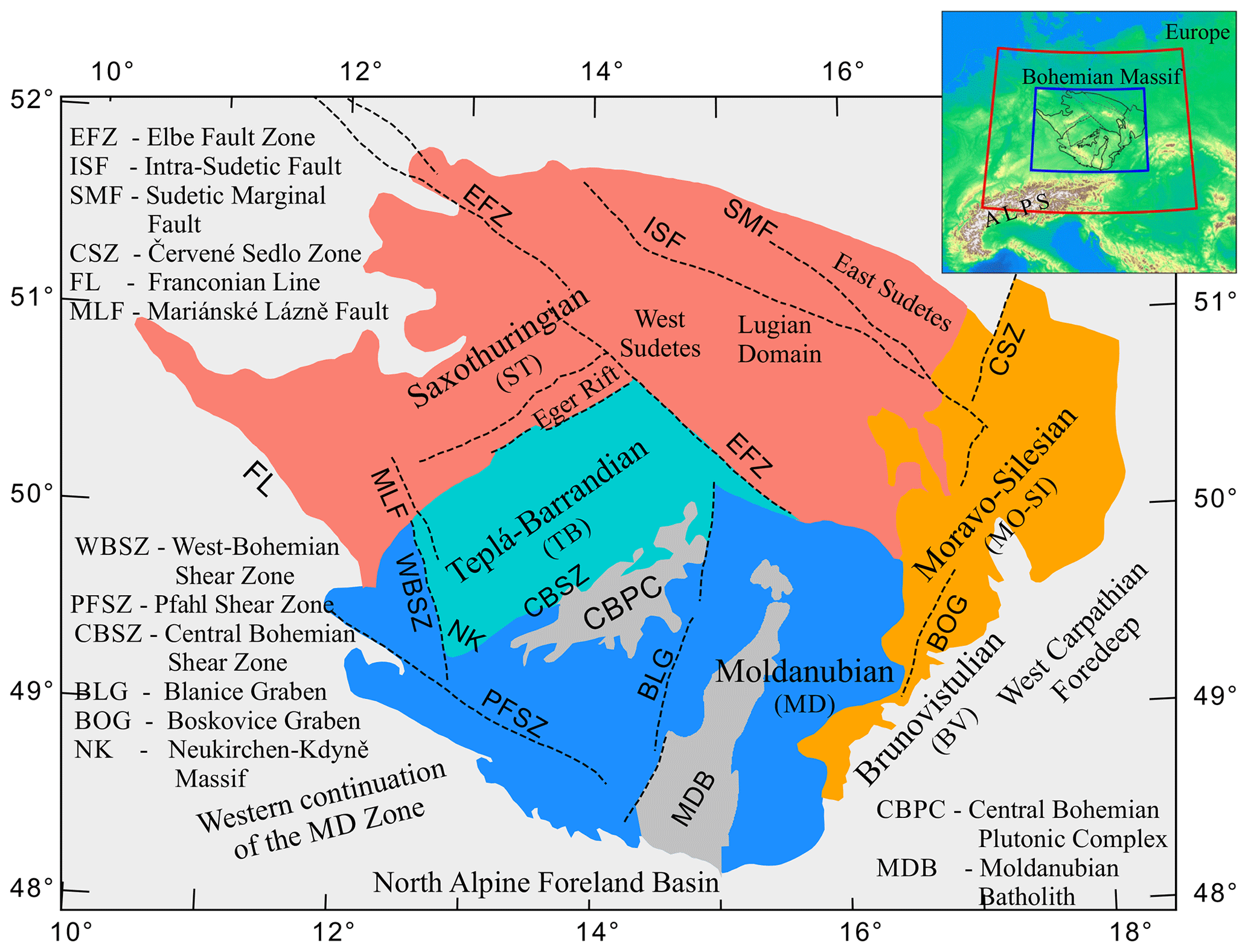
Figure 1Simplified overview of tectonic units of the Bohemian Massif (BM) and fault systems. The modelled region is framed in blue in the inset, and the red frame denotes the area of seismic stations used in the study.
Early controlled source seismic (CSS) research of the BM crust in the 1960s found the thickest crust of about 40 km in the MD unit and the thinnest crust (∼27 km) in the western part of the BM, in the ST unit (e.g. Beránek et al., 1975). The initial research was followed by many refraction and reflection seismic experiments that provided additional data for modelling the BM crust. Karousová et al. (2012, and references therein) interpolated the compiled findings of wide-angle refraction and near-vertical reflection seismic profiles into the first 3-D P-wave velocity model of the BM. The model maintains the gross features of the individual earlier models of the BM crust.
For a long time, active seismic experiments have represented the only source of data for studies of the BM crust due to the lack of natural earthquakes needed for local earthquake tomography of the massif. Complementary approaches, particularly the receiver function (RF) method (e.g. Hetényi et al., 2018b) and the more recently introduced ambient noise tomography (ANT) method, have been proven to be useful tools for imaging the crust. The former analyses delay times of converted phases from teleseismic earthquakes, and the latter is based on the cross-correlation technique (e.g. Bensen et al., 2007). The ANT method has the ability to model the Moho and to retrieve shear wave velocities across the Earth's crust and of the uppermost mantle when the network aperture is sufficiently large. One of the main advantages of the ambient noise tomography method is its ability to exploit long-term series of seismic ambient noise recorded at seismic stations regardless of earthquake occurrence and their spatial distribution. The resolution of velocity models most prevalently depends on station density, inter-station distance and azimuth variability, and the overall path coverage of the studied region.
In this paper, we present a homogeneous high-resolution 3-D shear velocity model of the entire BM crust, infer Moho depths, and map its lateral variations. The unprecedented high resolution of the velocity model is achieved thanks to data from temporary stations of the large-scale AlpArray passive experiment (Hetényi et al., 2018a) and several regional passive seismic experiments organised in the BM and its surroundings during the last 2 decades (see below).
We introduce a semi-automated procedure for ambient noise tomography, which consists of data-gathering, waveform preprocessing, calculation of station-pair cross correlations, the Rayleigh wave extraction, frequency–time analysis (FTAN), discretisation of the velocity dispersion curves of individual station pairs, and cross-dimensional dispersion curve tomography. The procedure leads to the homogeneous 3-D velocity model constructed from 1-D velocity–depth functions on a dense grid. The stochastic inversion with the use of the improved neighbourhood algorithm (Wathelet, 2008) provides several additional attributes, such as misfit, skewness, standard deviation, and estimates of uncertainty, allowing us to reliability assess the resulting velocity model. We compare the new 3-D model with several 2-D CSS profiles published by other authors and with estimates of the Moho depths using the RF method, resolved within this study. The velocity decrease modelled in the lower crust is explained by the vertical transverse isotropic (VTI) fabric with the “slow” symmetry axis.
To evaluate the shear velocities within the BM crust, we processed vertical components of daily recordings with a sampling rate from 20 to 200 Hz from 410 stations located in the massif and its broader surroundings framed from 46.2 to 56.3∘ N and from 7.1 to 21.4∘ E and operated between 2002 and 2016. We used recordings from permanent observatories, temporary stations of the AlpArray passive seismic experiment (AlpArray Seismic Network, 2015), its target-oriented complementary Eastern Alpine Seismic Investigation (EASI) field experiment (Hetényi et al., 2018b; network DOI: https://doi.org/10.12686/alparray/xt_2014), and recordings from previous temporary measurements in the BM, e.g. BOHEMA I-IV (Plomerová et al., 2007, 2012; Karousová et al., 2013), PASSEQ (Wilde-Piorko et al., 2008), and EgerRift (Babuška and Plomerová, 2013) (Fig. 2). Thorough analyses of noise sources showed that the 90 d interval in the summer season (from June to August) is the optimal time period for stacking cross-correlation functions in the BM (Figs. 3 and S1–S5). Strong microseismic energy arriving from the North Atlantic Ocean, particularly in the winter, greatly disturbs the ambient noise wave field in central Europe and, thus, corrupts the fundamental assumption that the method has an isotropic distribution of ambient noise sources. The summer season selection of data ensures similarity of the causal and acausal parts of the cross-correlation function (CCF; Fig. 3a, c) and the isotropy of the signal-to-noise ratio (Fig. 3a, b).
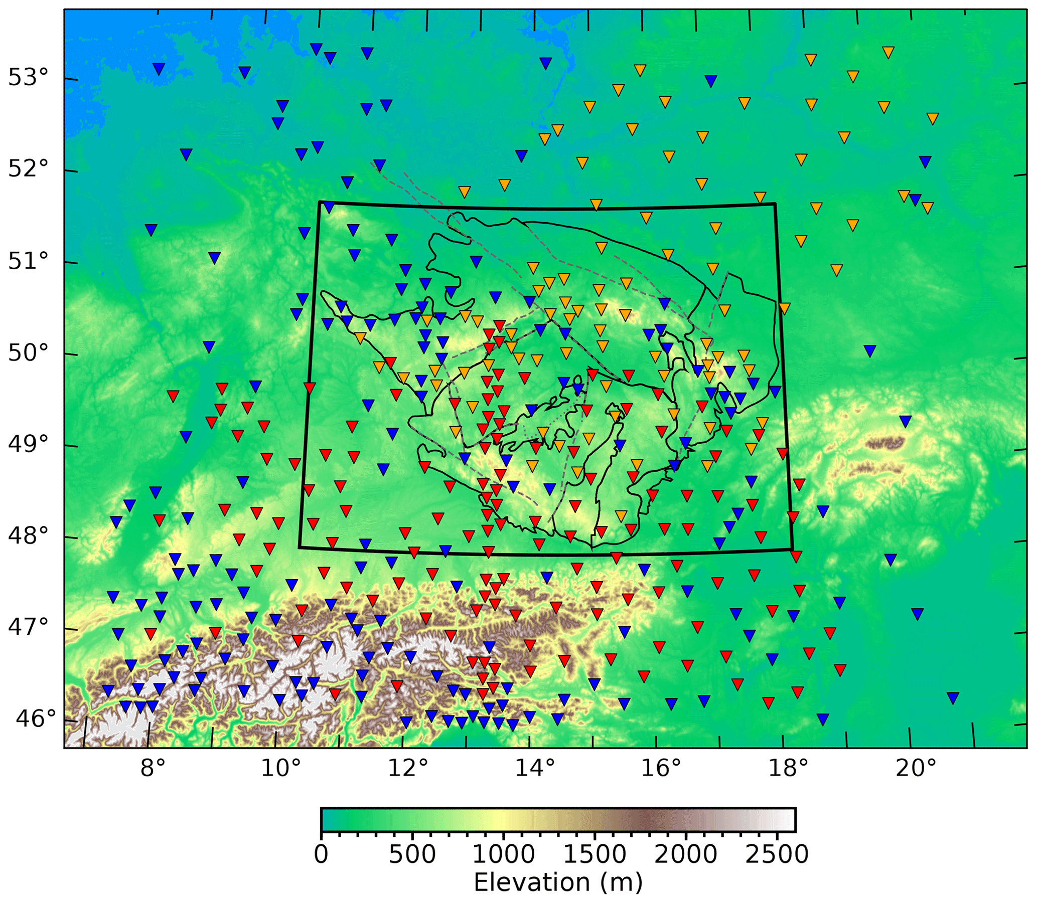
Figure 2Map of the AlpArray seismic stations (red), temporary stations from previous passive experiments (orange), and permanent (blue) stations available in the European Integrated Data Archive (http://www.orfeus-eu.org/eida, last access: 1 May 2021). The modelled region is framed, and the contours of geological units from Fig. 1 are shown.
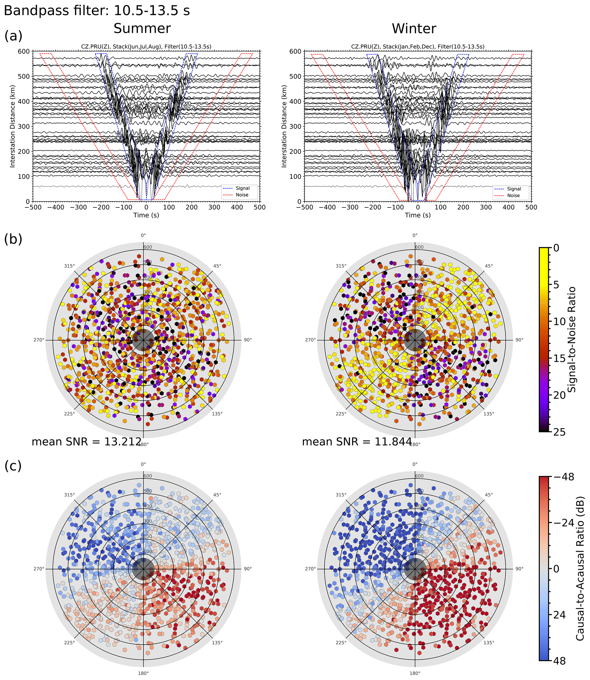
Figure 3Examples of cross-correlation functions (a) between data from station CZ.PRU and all permanent stations for the summer (left) and winter (right) months. The blue lines delimit windows used to measure the root mean square (RMS) amplitude of the coherent signal, and the red lines delimit windows used to measure the RMS amplitude of the non-coherent noise. Azimuth–inter-station distance rose diagrams present the signal-to-noise ratio (b) and the source directivity calculated as ratios of the causal and acausal parts of the CCF signals (c) for all permanent stations in the region for the winter and summer months (left and right diagrams respectively). The 10.5–13.5 s bandpass filter was applied before the analysis (Figs. S1–S5 present the same analyses with different bandpass filters). The CCFs and measurements in the rose diagrams that do not satisfy the minimal separation condition of the station pair for each period band are shown using grey and coloured shading respectively.
For our study, we created 83 845 station pairs from all of the available data and kept only those that satisfy the following conditions: the inter-station distance is between 50 and 600 km, the station-pair midpoint is inside the area framed from 47.5 to 52.4∘ N and from 11.3 to 19.3∘ E, and the station pairs contain at least 61 d of simultaneous recordings. Using these selection criteria, we retained 24 258 good-quality station-pair data suitable for ambient noise processing.
The framework for the calculation of surface wave velocity dispersion curves from ambient noise has been established in many theoretical (e.g. Dunkin, 1965; Lobkis and Weaver, 2001; Levshin and Ritzwoller, 2001; Sambridge, 1999; Yoshizawa and Kennet, 2005) and experimental studies (e.g. Shapiro et al., 2005; Yang et al., 2007; Ren et al., 2013; Kästle et al., 2018; Lu et al., 2018; Qorbani et al., 2020; Molinari et al., 2020). The studies are based on the cross correlations of long sequences of broadband seismic recordings and subsequent inversions of dispersion curves for shear wave velocity models. Among others, Lobkis and Weaver (2001) and Shapiro and Campillo (2004) showed that the cross correlations represent estimates of Green's functions for the crust and uppermost mantle along paths connecting two arbitrary sites. Reliable Green's functions can be retrieved if the medium is homogeneous and isotropic and if the ambient noise wave field is diffuse or arrives from uniformly distributed noise sources. However, none of these assumptions are fully satisfied in seismology. Therefore, additional processing is needed for modelling the structure of the crust. Bensen et al. (2007) describe data processing that delivers reliable surface-wave dispersion measurements, which are widely used in many of the recent studies mentioned above, even if the above-mentioned conditions are not fully satisfied. We have implemented this approach in building the first detailed 3-D velocity model of the BM. Due to the significant dispersion of surface waves as well as their frequency-dependent depth penetration, the surface wave tomographic inversion can be solved using a computationally efficient two-step approach. The two-step method integrates an iterative fast-marching method, resulting in shear velocity maps per frequency bands and a stochastic inversion of dispersion curves for a collection of multilayered shear velocity models. The stochastic inversion addresses a non-uniqueness of the formulae of Dunkin (1965) via a search for the best fit between the modelled and measured dispersion curves.
We build the 3-D shear wave velocity model in three semi-automated phases (Fig. 4) by joining three existing software packages. The MSNoise package of Python codes (Lecocq et al., 2014) is applied for data preprocessing, calculation of cross correlations, and their stacking in Phase 1. The package is complemented by a new set of Python codes for frequency–time analysis (FTAN) from Levshin and Ritzwoller (2001). This step includes careful velocity–frequency picking of the group velocity dispersion curves. The fast-marching surface tomography (FMST) package of Fortran codes (Rawlinson, 2005) is used to solve the 2-D surface wave travel time tomography in Phase 2. It employs eikonal equation forward modelling and the iterative subspace method to minimise the RMS error between the measured and computed travel times (Rawlinson and Sambridge, 2005). The non-linear stochastic inversion of dispersion curves (Wathelet, 2008) is solved in Phase 3 with the use of the Dinver software package (Wathelet et al., 2020). It employs the neighbourhood algorithm (NA) as an improved inversion method to search for the best-fitting models (Sambridge, 1999; Wathelet et al., 2004; Wathelet, 2008).

In Phase 1, we demean daily seismic records, resample them to a 0.1 s interval with an anti-aliasing filter, remove instrument responses, normalise amplitudes, and apply spectral whitening. We then compute daily cross-correlation functions (CCFs) for all station pairs by averaging cross-correlations computed for 1 h time windows with 30 min overlaps. We extract the fundamental mode of the Rayleigh waveforms and apply commonly used frequency–time analysis (FTAN). The FTAN diagrams (Fig. S6a) display amplitudes of waveform envelopes as a function of the group velocity and the period of narrow bandpass filters. On the FTAN diagrams, we measure group velocities of the Rayleigh waves. The group velocity dispersion curves are discretised efficiently by an automated picking with non-linear one-third-octave band segmentation of the frequency axis in the FTAN diagrams.
The automated picker starts from the third sample before the long-period cut-off point and continues in the direction of both the short and long periods. In the short-period band, the picker prioritises the low-velocity local maxima. This prevents picking the higher modes as well as skipping and mixing different phases in the short-period range. The cut-off period is a function of inter-station distance and average group velocity, and it relates to the separation of the causal and acausal parts of the Rayleigh wave on the CCF. By visual inspection of the FTAN diagrams, we reject 13 % of station pairs and end up with 21 066 dispersion curve measurements providing velocity–period pairs in a period range from 2 to 74 s (Figs. S6b, S25a).
In Phase 2, we split the whole set of station-pair dispersion curves and cluster the velocities according to the common periods. We convert measured group velocities into travel times and solve the travel time tomography using the fast-marching method (Rawlinson, 2005). Residual travel time RMS errors converge to the optimal velocity model after six iterations. The dense inter-station spacing allowed us to construct velocity maps at a grid of 0.1∘ N–S by 0.1∘ E–W. In the initial model, we use a constant velocity of 3.5 km s−1 and constant radius smoothing in order to avoid the introduction of artificial anomalies. Due to sparse ray-path coverage at longer periods, we increase the smoothing factor proportionally to each period with the aim of obtaining a smooth group velocity model without the appearance of the footprint of station pairs. Final group velocities for different periods along with roughness measures are shown in Figs. S7–S11. We construct Rayleigh wave group velocity models for the period range from 2 to 74 s in an area framed from 46 to 54∘ N–S and from 7 to 22∘ E–W.
In Phase 3, we assemble the velocity slices computed in Phase 2 and construct dispersion curves at a regular grid of 0.2∘ N–S by 0.3∘ E–W. We then invert the regularised dispersion curves in the range from 2 to 74 s for local 1-D layered shear velocity models with the use of NA in the stochastic inversion program. The reliability of the NA solution depends mainly on the number of randomly generated starting models, the number of iterations, and the model space. These parameters need to be carefully tested to guarantee the complete sampling of the solution space. The overall quality of the inversion results is assessed by misfit values, which indicate how each model fits the input dispersion curve by the normalised RMS error. We tune the NA parameters via evaluation of the misfit values, the coefficients of skewness (Kokoska and Zwillinger, 2000), and standard deviations of the group of best-fitting models with the aim of achieving the Gaussian distribution of group of best-fitting solutions without a bias of the NA search constraints.
The NA models consist of six-layers over a half-space (Table 1). The top three layers encompass the heterogeneous shallowest structures, and the three deeper layers represent the upper part and lower part of the crust and the uppermost mantle respectively. The NA searches for the best-fitting model in 360 iterations starting from 280 randomly generated initial models. To get a representative model at each grid node, we average 10 % of the best-fitting models from the resulting set of 400 000 models. We apply two approaches of averaging. The first approach is a conventional one that averages the vS over the fixed depths and results in a gradient velocity model (Fig. 5a–d, left panels, blue curves). The second approach averages over layer indexes (vi, zi) and results in a layered velocity model (Fig. 5a–e, left panels, red curves). This approach allows us to retrieve the velocity boundaries to which the surface waves are insensitive in principle. The dispersion curve, calculated from the layered velocity model, is a better match to the input dispersion curve (Fig. 5a, right panel). Therefore, we prefer the second way of averaging, and we build our final vS model from the above-mentioned 10 % of the best-fitting models.
Table 1Range of parameters for the neighbourhood algorithm (NA) stochastic inversion.
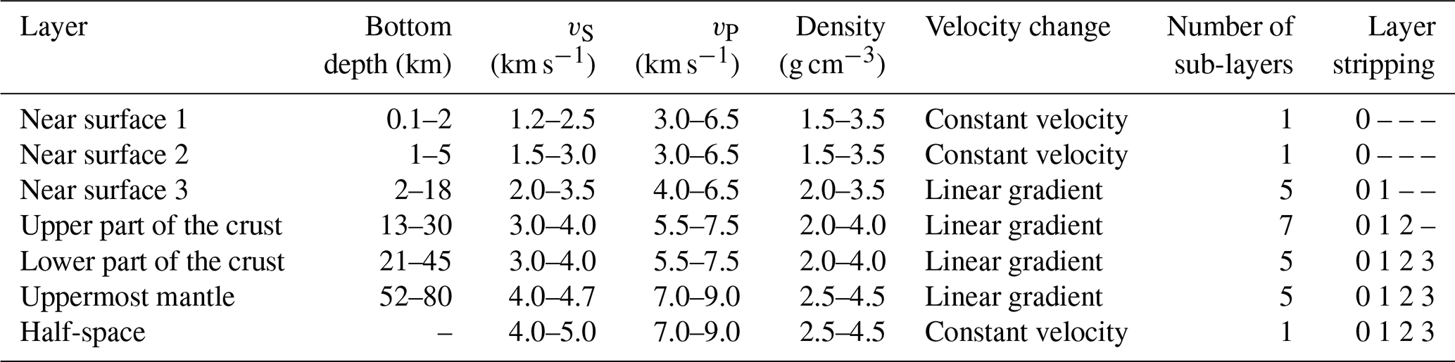
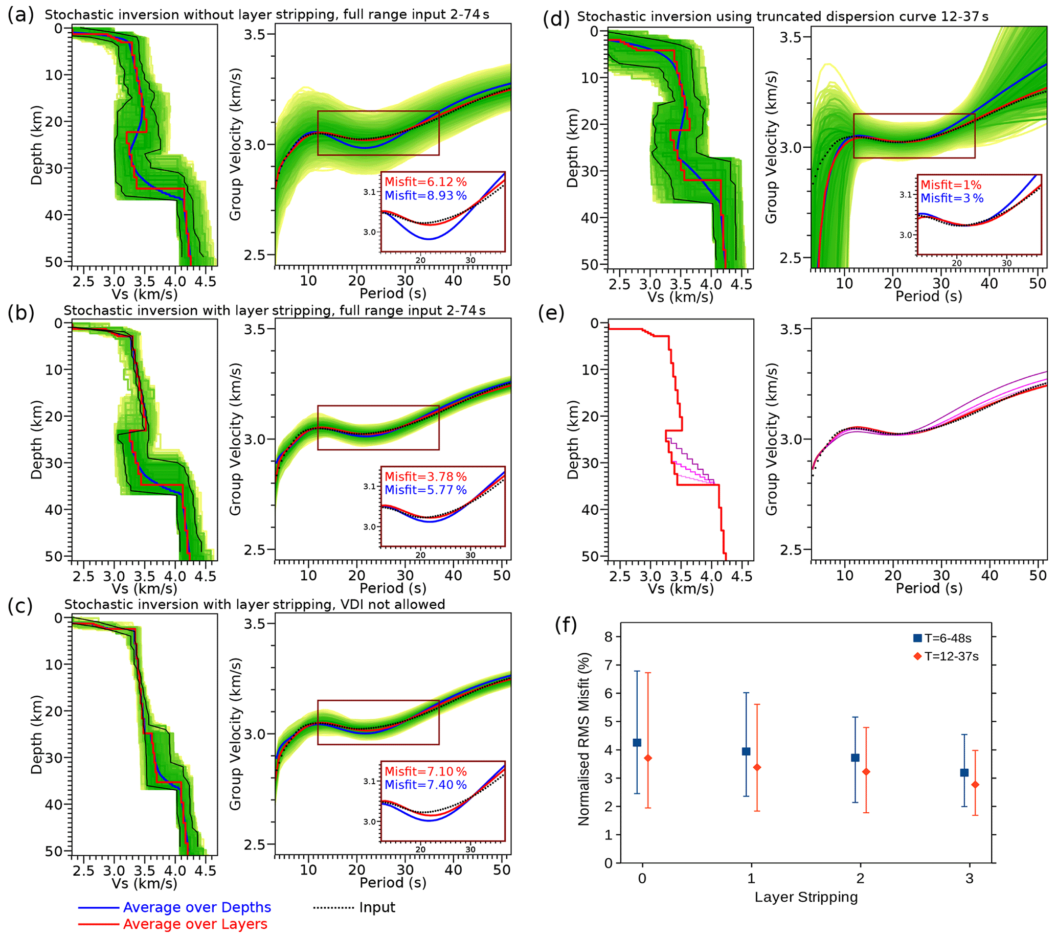
Figure 5Examples of dispersion curves at 50.7∘ N, 14.4∘ E for velocity models computed with different parameters. In panels (a–d), dispersions from models averaged over fixed depths are blue, and those from models averaged over layer indexes (xi, zi) are red. Individual parts of the figure show dispersion curves from models calculated without (a) or with (b, c) successive layer stripping from models where a velocity decrease was allowed (a, b) or was not allowed (c) during the inversions and from models resulting from inversions of the full-range dispersion curve (a) or the dispersion curve truncated at the 12–37 s interval (d). The misfit values are computed for parts of dispersion curves between 12 and 37 s, and the colour represents the method of velocity model averaging. For more details, see the text. Tests of a gradational Moho against a sharp Moho (e) limit the thickness of the potential transitional layer to 2 km. The yellow to green field marks 10 % of the best-fitting models from 400 000 computed models, with the thin black lines framing 1 % of the best-fitting models. The first quartile, median, and the third quartile display misfits between the input dispersion curves and those computed for all of the final 1-D models (see panel b, red curve) after each step of layer stripping (f) in period ranges of 6–48 and 12–37 s (blue and orange respectively). The misfit improves linearly with each run of layer stripping.
Averaging over layer indexes leads to the straightforward implementation of a layer-stripping technique in the stochastic inversion. Layer stripping appears to be efficient tool to enhance the NA search in deeper layers of the model, where the solution suffers from a significant decrease in sensitivity kernels with depth (Yoshizawa and Kennet, 2005). The recursive stripping of the upper layers increases depth sensitivity and leads to a better fit for the long period range of the dispersion curves (Fig. 5b). Figure 5f reveals the linear improvement of the average misfits for two selected period intervals, after each of the three steps of the subsequent layer stripping. The misfit reduction is feasible and consistent for all nodes.
Similar improvement concerns setting the inversion parameter that allows or does not allow the velocity decrease in the lower part of the crust. Figure 5b and c show an example of the inversion results at a site where velocity decrease with depth (Fig. 5b) needs to be allowed in order to achieve a better fit for the dispersion curves exhibiting a local minimum around the 20 s periods. In our data set, a large majority of the resulting models consistently prefer the velocity decrease in the lower crust (see also Fig. 8). In order to further verify the sensitivity of our layer-stripping method to the velocity decrease feature in the lower crust, we invert the dispersion curves truncated at the mid period range from 12 to 37 s, which is sensitive to the lower crust and contains the local minimum. Although the misfits with the truncated input are lower, the models fail to fit the dispersion curves outside the truncation frame (Fig. 5d, right panel). Regardless of whether the inversion is computed with or without layer stripping, or from a full or truncated window of dispersion curves, the resulting models end up with the velocity decrease feature in the lower part of the crust (Fig. 5a, b, d), if the model space allows for such a velocity decrease.
We assess the sensitivity of our inversion approach to the sharpness of the Moho as an interface by adding an additional gradient layer into the final 1-D model (Fig. 5e). In order to mimic the gradational Moho, we insert the layer on top of the uppermost mantle layer (Table 1) and vary its thickness from 2 to 10 km. The test shows that the larger the thickness of the transitional layer, the worse the misfit in the dispersion curves, which is detectable from a layer thickness larger than 2 km. This means that in the case of the gradational Moho instead of a sharp discontinuity, the thickness of the transitional layer does not exceed 2 km.
The presented high-resolution model shows shear wave velocities that are ∼0.2 km s−1 higher in almost the entire BM upper crust, on average, than those in its surroundings, with the highest velocities in the southern part of the Moldanubian (MD) unit (Fig. S12). The higher velocities clearly contour the BM shape. Very low velocities down to a depth of 10 km mark the south-east rim of the BM beneath the Carpathian Foredeep. At greater depths (15 km), the relatively higher velocities are found in the MD unit. Locally increased velocities occur in the lower crust in several places, such as beneath the Eger Rift (ER) at a depth of 25 km. The upper-mantle velocities arise first in a 28 km depth slice beneath the Eger Rift, thereby marking the massif thinning along the rift. While we find the top of the upper mantle at 32 km in the Saxothuringian (ST) unit, it is as deep as 39 km in the MD unit.
Figure 6 shows depths of the Moho discontinuity, as an interface between the last sub-layer of the lower part of the crust and the first sub-layer of the uppermost mantle (see Table 1), across which the lower-crust velocities change into the upper-mantle velocities. The crust of the BM is thinnest in its Saxothuringian part, beneath which the upper-mantle velocities dominate at a depth of ∼32 km, with very thin crust beneath the ER (∼28 km). The ambient noise tomography detects the thickest crust beneath the Moldanubian part of the BM, where the Moho deepens to at least ∼38 km. The Moho has been detected as deep as 36 km in a small area around the boundary of the West Sudetes and the Lugian Domain around the Intra-Sudetic Fault (ISF).
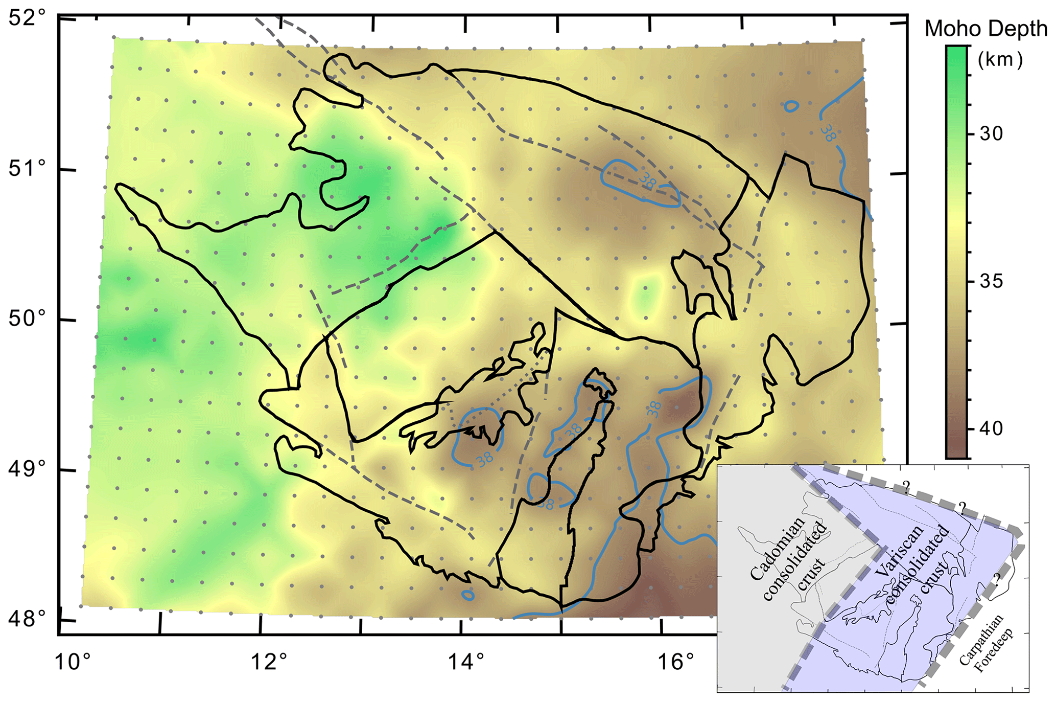
Figure 6Thickness of the BM crust from ambient noise tomography. The Moho discontinuity is modelled as the interface between the last sub-layer of the lower part of the crust and the first sub-layer of the uppermost mantle (see Table 1). The Moho depths of 38 km are contoured. For standard deviations and skewness coefficients of the Moho depths, see Fig. S13.
Regardless of the shallowest, not well-resolved upper 3 km, the model comprises two well-resolved layers, which we relate to the upper and lower parts of the crust (UPC and LPC in Fig. S14 respectively). In the UPC, the average velocities vary from ∼3.2 km s−1 in the north and north-west of the massif up to more than 3.5 km s−1 in the southernmost part of the BM. With two small exceptions (along the Boskovice Graben and Lugian/Moravo-Silesian contact), the LPC of the BM can be divided into south-western and north-eastern halves, exhibiting relatively high and low average velocities respectively.
The 1-D velocity–depth models, resulting from the stochastic inversions, exhibit distinct regional variations in the velocity interface between the LPC and UPC, which are characteristic of individual tectonic units of the BM (Fig. 7; for their corresponding dispersion curves, see Fig. S15). Comparison of 1-D models with the radial Earth model IASP'91 (Kennet and Engdahl, 1991) shows that the shear velocities retrieved in the upper part of the crust are mostly similar, whereas the ANT model velocities are significantly lower in the lower part of the crust.
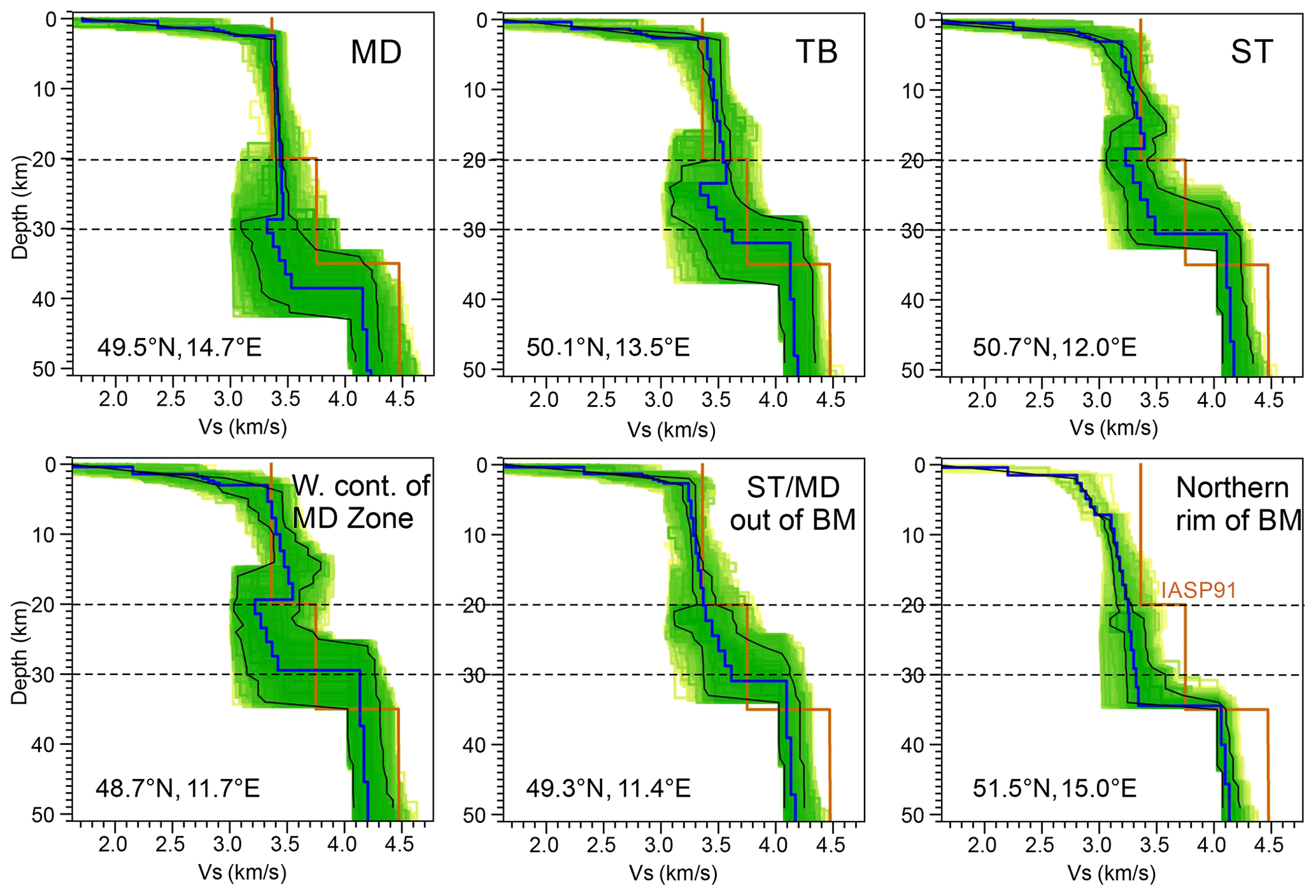
Figure 7Examples of vS models, characteristic of individual tectonic units (for the abbreviations, see Fig. 1 and the text). The blue curve is the average model calculated from 10 % of the best-fitting models from the 400 000 models in total (yellow to green curves). The thin black curves frame 1 % of the best-fitting models. The corresponding dispersion curves are shown in Fig. S15.
Most of the massif is characterised by a velocity decrease in the lower crust, which can be quantified as , where indexes denote respective sub-layers (Table 1). The velocity-drop interface (VDI) with negative dvS occurs at variable depths and with different-sized velocity drops (Fig. 8). Within the MD, the interface with a velocity drop exceeding −0.1 km s−1 lies between a depth of 26 and 30 km and is deepest in the south, although the average velocity decrease is not the largest one (49.5∘ N, 14.7∘ E; depth = 28 km; km s−1). The MD is surrounded by a band in which the VDI uplifts into shallower depths. In the south-west continuation of the MD unit out of the BM (see Fig. 1), the size of the velocity decrease becomes even stronger locally, but the depth of the interface shallows by ∼10 km (48.7∘ N, 11.7∘ E; depth = 19 km; km s−1). The amplitude of the negative dvS also slightly increases towards the TB unit, but its depth remains deeper than that in the westward continuation of the MD unit out of the BM (50.1∘ N, 13.5∘ E; depth = 23 km; km s−1). The south-west–north-east trend of the Variscan structures, including the ER, is reflected in a separation of the ST, characterised by the weaker velocity decrease across the VDI at shallower depths (50.7∘ N, 12.0∘ E; depth ∼18 km; km s−1) in comparison with the rest of the BM. In the south-western part of the region (49.3∘ N, 11.4∘ E), where the ST unit neighbours the crust of the MD zone (out of the BM), the VDI is absent. The narrow zone without the velocity drop continues north-eastward along the ER (ST–TB boundary). Further to the north-east, the ER continuation approximately divides the regions with a shallow and deep VDI in the West Sudetes and the Lugian Domain respectively. The VDI is a little bit more expressed around the Elbe Fault Zone (EFZ) and lies deeper to the north-east of the EFZ in comparison with the ST south-west of the EFZ, but it remains shallower in comparison with the MD. Further to the east in the northern BM, the VDI deepens to ∼25 km in the northern Lugian Domain and shallows again to ∼20 km in the Silesian (Fig. 8).
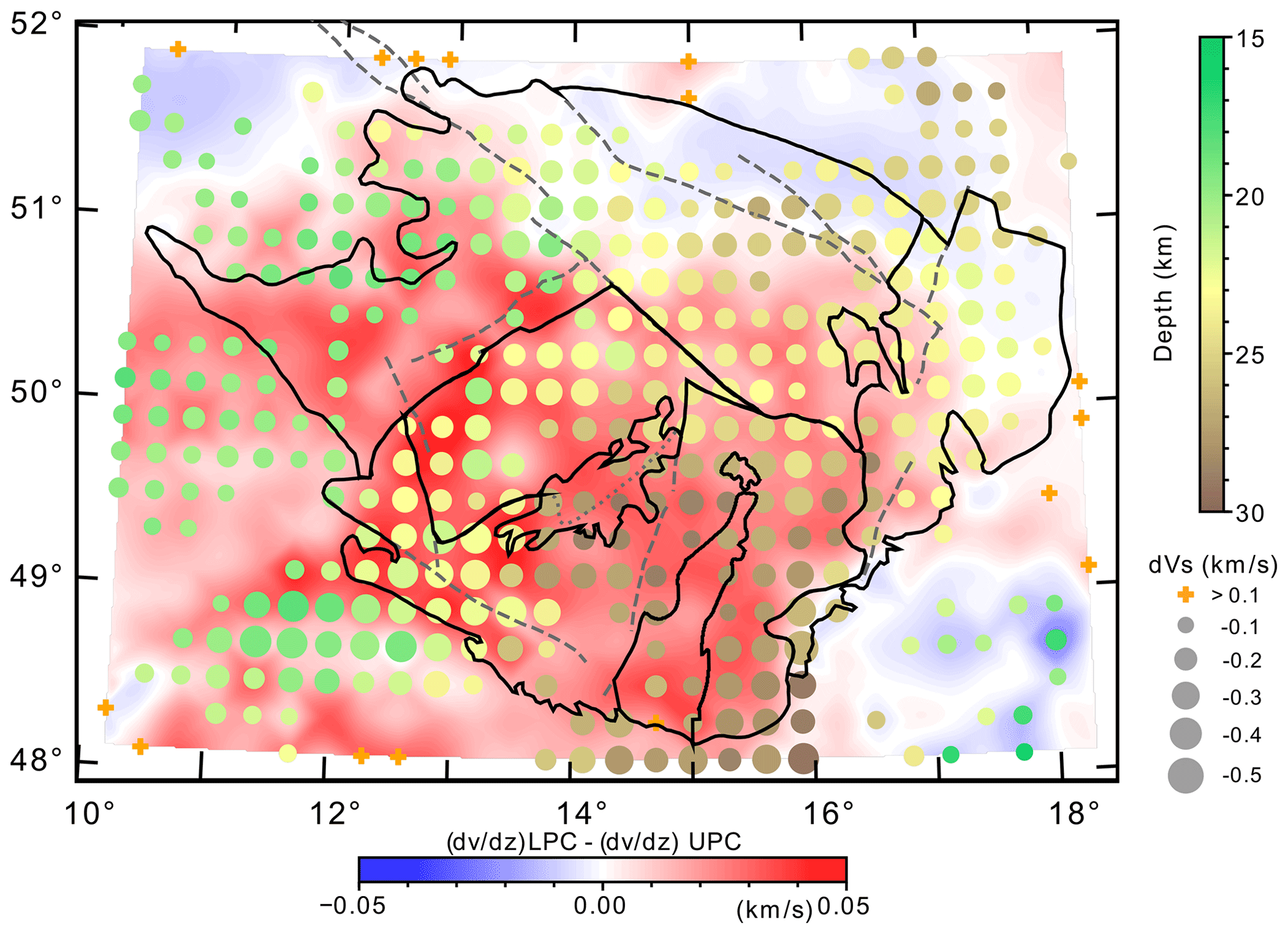
Figure 8Depth of the velocity-drop interface (VDI) along with differences in velocity gradients (coloured background) in the upper and lower part of the crust (UPC and LPC respectively). The circle size is proportional to the amplitude of the velocity drop across the VDI. The UPC–LPC boundary is an interface between the last sub-layer of the upper part of the crust and the first sub-layer of the lower part of the crust (see Table 1). For standard deviations and skewness coefficients of the UPC–LPC interface, see Fig. S16. Note the deeper VDI in the Moldanubian and Brunovistulian units with the thick crust.
Besides the tiny but systematic differences between average velocities in the upper and lower crust (Fig. S14), there are also differences in the velocity gradients in the individual regions of the BM (Fig. 8). The EFZ divides the BM approximately into two zones. The southern zone of the BM, which includes the MD and TB units, the eastern ST unit, and southern part of the Lugian Domain, is characterised by higher velocity gradients below the VDI than that in the layer above the VDI. In the north-eastern rim of the BM, particularly north of the ISF, in the East Sudetes and Silesian Domain, the gradient difference at VDI is negative, i.e. the gradient in the layer above the VDI is higher than that below the interface. The differences between velocity gradients in the UPC and LPC clearly delineate zones of the BM that match with the BM zonation according to the size and depth of the velocity drop at the VDI (Fig. 8).
Distinct lateral variations in the vS velocities, the VDI, and the Moho depths, as well as thickness of the LPC are shown along several cross sections in the 3-D view (Fig. 9; for more views, see Figs. S17–S20). The sharp dark blue–light green velocity contrast marks the Moho derived from ambient noise tomography. The figures show crustal thinning, e.g. beneath the ER (Fig. 12), and Moho undulations, e.g. around the crossing point of Profile 7 and Profile 12 beneath the southern SI (eastern continuation of the EFZ). The shallow Moho beneath the ST unit is also visible along Profile 14 (south-western part viewed from the south-west).
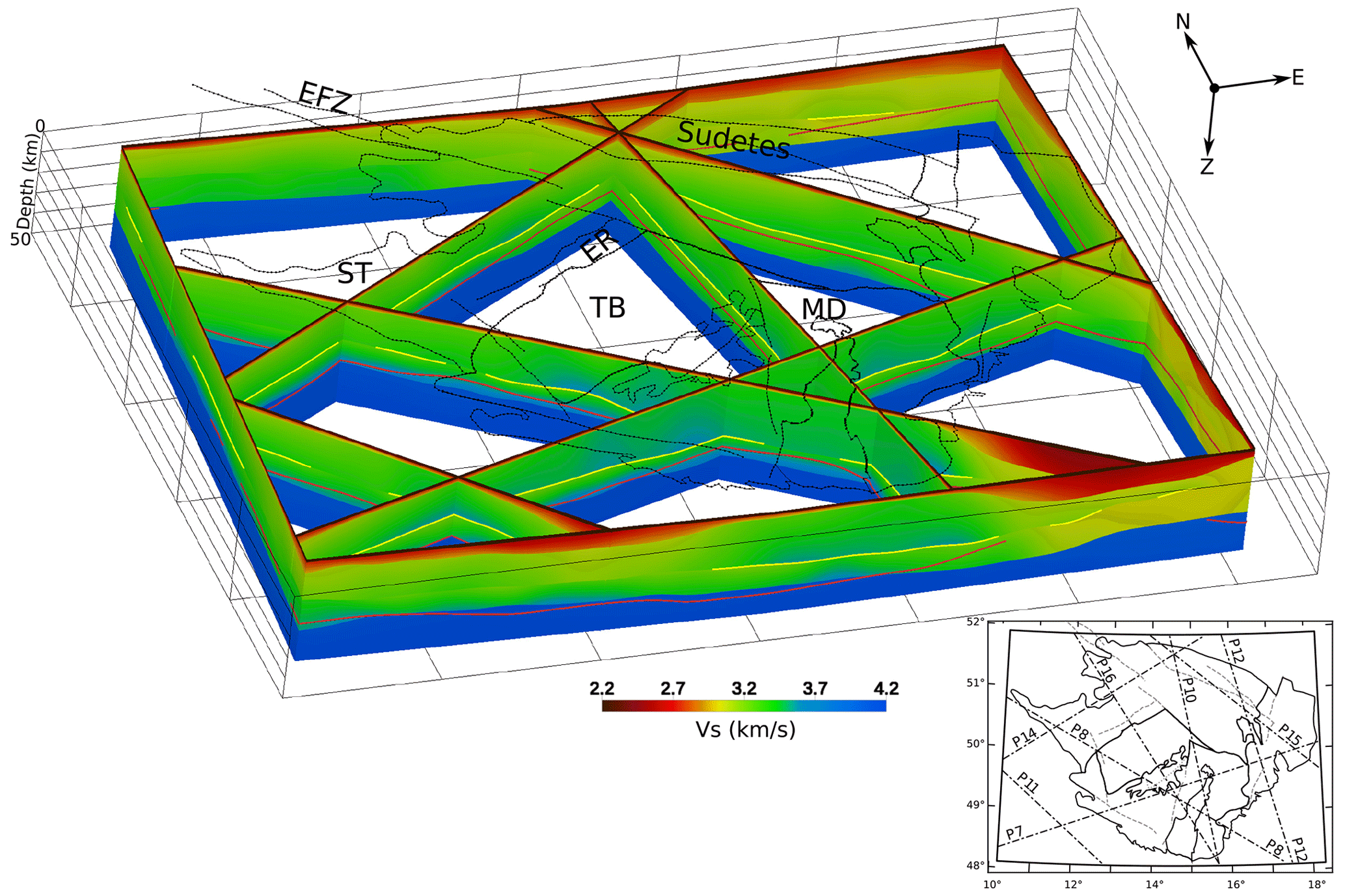
Figure 9A 3-D view of the vS ANT model of the BM from the south-west. The yellow segments denote the velocity-drop interface (VDI) at sites with a velocity decrease of at least −0.1 km/s. The Moho depth estimated from the Ps–P delay times in receiver functions calculated in this study for all the stations is shown in red. Profile locations and names are shown in the inset. The depth scale is exaggerated. For more views, see Figs. S17–S20.
The Ps receiver functions represent an independent method to estimate the Moho depth from teleseismic P-to-S converted phases at the bottom of the crust. We picked the Ps–P delay times for all the stations and calculated the Moho depth with the use of the IASP91 velocity model (for more details, see Hetényi et al., 2018b). We interpolate the Moho depth estimates beneath individual stations without the back migration to true conversion points. In the core of the BM (the TB and the south-western part of the MD units), the Moho depths from the time delay of the Ps-converted phases (MohoRF) and from the ambient noise tomography (MohoANT) are in agreement. In the remaining part of the BM and the Carpathian Foredeep, the MohoANT is deeper, except for the very southern MD. The most frequent difference between the MohoANT (Fig. 6) and MohoRF (Fig. S21) is 3 km over the whole region (Figs. S22 and S23). The Moho depth estimated from the Ps–P delay times with the use of the average crustal vS from our ANT model (vANT) and standard is even shallower. The most frequent value is almost 4 km. This reflects the velocity decrease in the LPC in most of the BM velocity models, which shallows the Moho estimates from RF, on average, if standard from the IASP'91 is used. Aiming to attain the same Moho depth as in the ANT model (MohoANT) requires a that is 0.15 lower than that corresponding to the IASP'91 model or the from the Zhu and Kanamori method (2000) retrieved from the same data set. There are clear regional variations (Fig. S24) which relate mostly to velocity variations in the LPC.
Mostly in the northern and eastern parts of the BM, the Moho depths differ more than would correspond to the estimated accuracy of km (e.g. Fig. 9, Profiles 10, 14, and 15, and Figs. S17–S20). Exceptional large discrepancies occur in regions south-east of the BM, with sediments not compensated for in MohoRF calculations. Lower average velocities in the ANT model shallow the Moho depth estimates from the RF by 1 km on average, relative to estimates if the IASP'91 velocities are used.
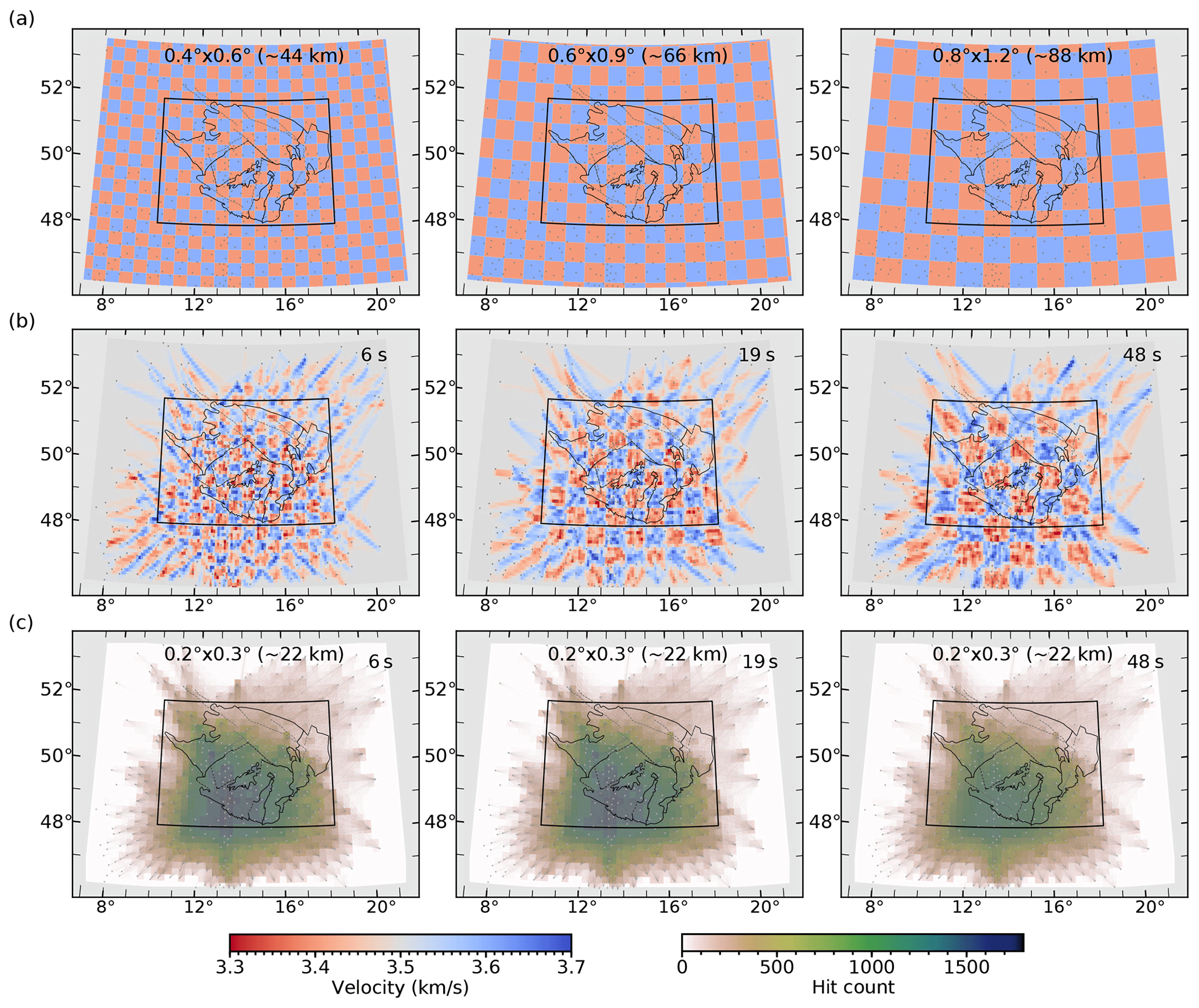
Figure 10Checkerboard tests (b) calculated for models with cell sizes of 0.4∘ N–S by 0.6∘ E–W, 0.6∘ N–S by 0.9∘ E–W, and 0.8∘ N–S by 1.2∘ E–W (a) for ray-path coverages at periods of 6, 19, and 48 s. The level of Gaussian noise added to the synthetic travel times corresponds to 50 % of velocity variations in the synthetic velocity models (a). (c) Hit counts express the numbers of rays crossing each cell centred around a 1-D inversion grid of 0.2∘ N–S by 0.3∘ E–W .
The most distinct phenomenon of the presented model is the detection of the velocity-drop interface (VDI) in the lower crust with the velocity decrease exceeding −0.1 km s−1 (marked by yellow lines in Figs. 9 and Figs. S17–S20). Variations in both the interface sharpness (size of the velocity drop) and its depth change laterally. These changes can be related to individual tectonic units of the BM crust (see Figs. 7 and. 8,). On the other hand, there is no direct correlation between the Moho, or the VDI depths, and the lower-crust thickness. Although the thin and thick lower parts of the crust beneath the VDI are visible above the deep and shallow Moho respectively (e.g. P16, view from the west), the reversed relation, i.e. the thin and thick LPC above the shallower and deeper Moho respectively, can be seen as well (e.g. P10, view from the west, or P14, view from the east). This may reflect the fact that the accuracy of determining both the Moho and VDI depths is not sufficient to quantify the subtle relationship between the thickness of LPC and Moho depth.
We use standard synthetic checkerboard tests to assess the resolution of the fast-marching tomographic inversions. We search for spatial resolution in checkerboard patterns with a % velocity perturbation relative to the initial velocity model (3.5 km s−1) and with three cell sizes (Fig. 10a). We add Gaussian noise to the synthetic travel times, before the FMST inversion, to simulate uncertainties in the dispersion curve-picking procedure. As expected, the spatial resolution relates to the ray-path coverage for each period. In the central and southern parts of the model, we retrieve velocity heterogeneities at a size of 44 km by 44 km using a ray-path coverage at the 6 s period (Fig. 10a and b, left), 66 km by 66 km at the 19 s period (Fig. 10b, centre), and 88 km by 88 km at the 48 s period (Fig. 10b, right). The resolution decreases towards the northern part of the model and towards the model margins with sparse ray-path coverage. The ray-path coverage of the region is shown in Fig. 10c by the ray-path hit count per 0.2∘ N–S by 0.3∘ E–W cell size.
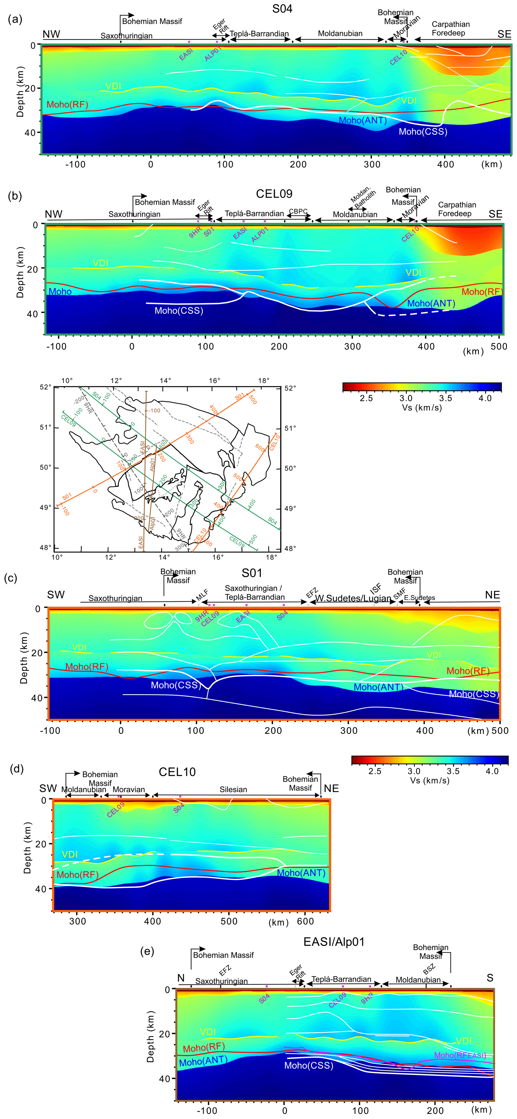
Figure 11Cross sections through the 3-D vSANT model (coloured background) along five CSS profiles. White lines mark velocity boundaries according to the ALP01 (Brückl et al., 2007), CEL09 (Hrubcová et al., 2005), CEL10 (Hrubcová and Środa, 2008), S01 (Grad et al., 2008), and S04 (Hrubcová and Środa, 2010) CSS models (see inset for locations). The Moho depth, estimated from the Ps–P delay times in receiver functions calculated in this study for all of the stations, is shown in red. The magenta line in panel (e) is the Moho along the AlpArray–EASI by Hetényi et al. (2018b). The vertical scale of the cross sections is exaggerated at 3:1.
Further, we verify the reliability of the fast-marching inversion at different periods based on travel time residuals computed for all input travel paths through the updated 2-D velocity slices. The travel time residuals document that the FMST inversion returns a reliable solution in a period range from 6 to 48 s (Fig. S25b). The computed travel time residuals at short periods (<5 s) significantly exceed the short wavelengths due to the increased uncertainty of the dispersion curve picking. Therefore, the fast-marching inversion does not provide reliable results for short periods. The lower reliability of the fast-marching inversion for long periods (60 and 74 s) is affected by the reduced number of the travel time inputs into the inversion (Fig. S25a).
Finally, we also calculate the depth sensitivity kernels at each cell of the final velocity model and demonstrate their well-known dependence on period (Fig. S25b). The average sensitivity kernels, calculated across cells in the BM, show the highest sensitivity to structures in the upper part of the crust (∼3–20 km) for periods between 6 and 19 s. The lower part of the crust down to the Moho is sampled well with periods >19 s. To estimate the vertical resolution of our final vS model, we use standard deviations of 10 % of the best-fitting models. The skewness coefficients provide confirmation that the model space in the stochastic inversion is fully explored and that the model space does not influence the outcome. The skewness coefficients for the UPC–LPC boundary (Fig. S16) and the Moho (Fig. S13) are around zero and confirm that both interfaces are well explored. The standard deviations for the Moho and UPC–LPC depths are mostly below 3 and 5 km respectively.
Based on the resolution and sensitivity tests, we infer that the VDI – the new phenomenon retrieved in the presented model at a depth of ∼15–30 km – lies in a high-fidelity area for both the sensitivity kernels and minimum travel time residuals. Results of the spatial resolution tests confirm that we can resolve structures at least as small as ∼40 km in the upper part of the crust and ∼80 km in the lower crust in the velocity model from ANT.
Traditionally, the upper and lower crust are distinguished in velocity models of the Earth crust by higher velocities in the lower layer and the strong positive velocity contrast at the bottom of the crust (Moho). The mid-crust boundary, called the Conrad discontinuity, was originally supposed to separate the granitic and mafic crustal layers. However, the suggested Conrad discontinuity is missing in many seismological models with gradient velocities. In this paper, we show that an intra-crust boundary can appear with a negative velocity contrast in the lower crust.
The dispersion curves of group velocity computed by FMST in the BM are characterised by a steep slope of velocity increase in short period range <8 s. The curves have flat local maxima between the 10 and 15 s periods, followed by a subtle velocity decrease with local minima at ∼20 s and a moderate velocity increase for periods larger than 20 s. The general level of the local maxima of the dispersion curves attains group velocities of ∼3.1 km s−1. This value is lower than velocities from the steeply increasing dispersion curves of Lu et al. (2018) in the BM. However, the general shape and velocity level of our dispersion curves are comparable to those of Ren et al. (2013), Shippkus et al. (2018), Qorbani et al. (2020), or Molinari et al. (2020). Also, the ANT models of these authors show a higher vS in the BM upper crust than in its surroundings.
Wide ranges of 1-D layer thicknesses and velocities in our ANT input parameters (see Table 1) result in a vS model of the BM crust with three characteristic depth zones. The uppermost part, thinner than 3 km, is not well resolved due to locally heterogeneous structures including sediments in some places. For the two main parts of the crust, we use the same notation as that introduced by Artemieva and Thybo (2013) in their EUNAseis seismic model for Moho and crustal structure in Europe derived from a compilation of CSS and RF models. The upper part of the crust (UPC) includes felsic material with P velocities of 5.6–6.4 km s−1 and the middle crust with intermediate composition and velocities of 6.4–6.8 km s−1. The lower part of the crust (LPC) denotes the mafic lower crust with velocities of 6.8–7.2 km s−1 and the high-velocity lowermost layer with vP higher than 7.2 km s−1.
However, contrary to the commonly observed P-velocity increase with depth, we retrieved lower shear velocities in the LPC than in the lower part of the UPC. No mid-crust layer or an interface with positive impedance (traditional Conrad discontinuity) is required in our gradient velocity model. The characteristic velocity-drop interface (VDI) between the UPC and LPC can be associated with a thermodynamically controlled interface or rheological boundary representing the modern view of the Conrad discontinuity (Lay and Wallace, 1995).
6.1 BM crust images in ANT and CSS
Several CSS profiles criss-cross the BM (Fig. 11) and allow us to compare the characteristics of the velocity cross sections through the 3-D ANT vS model with the 2-D vP models from series of the CSS measurements. To do so, we superimpose the vS velocity model onto the main features of the CSS profiles, especially onto the Moho discontinuity and inter-crustal boundaries.
Two parallel CSS profiles, Sudetes S04 (Hrubcová et al., 2010) and Celebration CEL09 (Hrubcová et al., 2005), cut across the Variscan structures in the BM. While the Moho depths in central parts along the CEL09 profile and the ANT cross section overlap (∼150–300 km of the profile, Fig. 11b), the MohoCSS along the S04 is 6 km shallower than the MohoANT, (∼100–300 km, Fig. 11a). The MohoRF follows the shallower MohoCSS relief there and remains shallower along the CEL09. The MohoRF in this area could be associated with the top of a layer with higher velocities in the lowermost part of the LPC (Artemieva and Thybo, 2013). The Moho depth differences increase in the south-eastern parts of both profiles (∼400–500 km) due to sediments in the Carpathian Foredeep. Laminated high-vP gradient layers, modelled in the north-western and south-eastern parts of the CEL09, fit neither the sharp MohoANT nor the MohoRF. The RFs are primarily sensitive to a velocity contrast across the interface, although locally higher or lower crustal velocities affect the depth-migrated Ps delay times accordingly. None of the intra-crustal boundaries marked in the S04 or CEL09 profiles correlate with the distinct VDI in the ANT vS model. Majdanski and Polkowski (2014) estimate uncertainties in velocities, as well as interfaces in the CSS models, and show significant variations for deeper layers. According to their analysis, the MohoCSS lies in a 9 km broad interval in the marginal segments of the CEL09 profile, as a bottom of the high-gradient velocity layer with a velocity uncertainty of ∼0.4 km s−1. An even larger uncertainty of ∼0.6 km s−1 is estimated for P velocities modelled in the uppermost mantle.
Similar features exist in the S01 (Grad et al., 2008) and CEL10 (Hrubcová and Środa, 2008) profiles, both of which parallel the north-east–south-west trend of the BM tectonics. Up to 5 km differences in the shallow MohoCSS and the MohoANT exist northward of the EFZ, and these differences are even larger for the MohoRF locally. Two small high-velocity narrow blocks in the upper crust (∼50–200 km, S01; Fig. 11c) are localised close to the higher velocities in the ANT model. A complex 2-D image of the Moho structure modelled beneath these two high-velocity blocks in the S01 profile is missing at the crossing point in the CEL09 profile (∼100 km; Fig. 11b), which indicates that the existence of the corresponding 3-D feature is improbable. The largest uncertainty in the MohoCSS depth of ∼5 km is estimated beneath these two upper-crustal structures, and it is high in the whole central part of the profile (Majdanski and Polkowski, 2014). A high-velocity gradient zone of large extent is modelled along the CEL10. This zone correlates with the model of the laminated Moho at the crossing point with CEL09. However, there is no laminated Moho on S04 at the crossing point with CEL10. Tests of the sharpness of the Moho in the ANT model at the two crossing points do not indicate a laminated Moho thicker than 2 km (Fig. S26). Instead, the localised high-velocity lowermost crust occurs around both crossing points (CEL09 × CEL10 and CEL10 × S04) in the 3-D ANT velocity model (see Fig. 11a, d).
Table 2Models of the crust beneath the KHC station (Moldanubian unit).
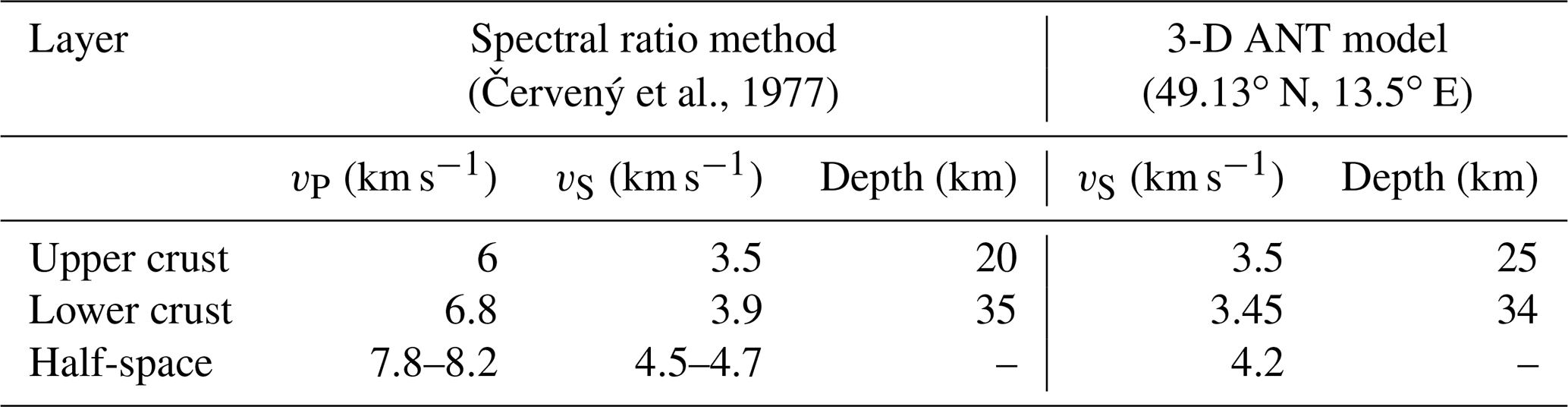
The Moho depths from different data sets and the three independent techniques fit best along the ALP01 north–south profile (Brückl et al., 2007) and the AlpArray-EASI (Hetényi et al., 2018b) running through the BM (Fig. 11e). In general, discrepancies in the Moho depth determination of less than 5 km, which is the most frequent case for the BM, are considered as a good match (Kästle et al., 2018). We also found a good fit with the two-layer model of the crust beneath the KHC station (49.13∘ N, 13.58∘ E), located near the AlpArray-EASI, ALP01 (∼150 km) and 9HR CSS profiles (Červený et al., 1977). The authors applied the spectral ratio method by Phinney (1964) to data from the first European stations, which have provided continuous broadband digital recordings since 1972 (Plešinger and Horálek, 1976). The preferred two-layer model, with constant velocities, sets the Moho at 35 km, which is in agreement with both CSS results and the ANT model presented here (Table 2). However, the upper–lower crust boundary is 5 km deeper in our model. While the velocity gradient in the upper crust is also constant in our model, we found a 0.2 km s−1 vS decrease at the VDI and a relatively steep positive velocity gradient in the lower crust. The velocity remains lower even at the bottom of the crust (vS=3.6 km s−1). The uppermost mantle velocities are lower in the ANT model than those derived from the dispersion curves of teleseismic Rayleigh waves for the half-space by Červený et al. (1977). Waves in that model arrived from back-azimuths of ∼30∘, which is close to the high-velocity directions derived from body-wave propagation of regional earthquakes (Plomerová et al., 1984). The ANT model presented in this paper accounts for dispersion curves from all directions, which decreases the velocities (see Table 2). An intra-crustal boundary in ALP01 (Fig. 11d) follows the VDI interface, similarly to that in CEL10, where it coincides with the top of the positive high-vP-gradient transitional layer. In this case, the results from the trial-and-error technique of 2-D modelling of the wide-angle CSS data differ from results obtained from the 3-D ANT, which modelled relatively low vS velocities in the LPC and the sharp Moho.
When comparing results from the CSS and 3-D ANT, one has to be bear in mind that the 2-D CSS models are significantly affected by 2-D processing assumptions and narrow azimuth data acquisition, whereas the 3-D ANT model is based on 3-D homogeneous sampling and imaging of the crust, although with a relatively lower resolution in the lower crust. Therefore, the ANT method can image 3-D structures of the crust in a more realistic way compared with the case when the 2-D CSS lines do not match at crossing points. Thanks to layer stripping and the model averaging method, the ANT model reveals the Moho as a sharp discontinuity beneath the whole BM. However, the mantle velocities beneath the Moho remain lower than expected. Nevertheless, the lower velocities are in agreement with the ANT results of Ren et al. (2013), the teleseismic body-wave tomography results of studies such as Amaru (2007), Plomerová et al. (2016), and reference therein, and the full wave-form inversion results of Fichtner and Villasenor (2015). The shear velocities in the upper crust are in agreement with the vP CSS models considering the standard ratio. An apparent inconsistency occurs in the LPC, where ANT models a decrease in vS from the dispersive group Rayleigh waves, whereas the CSS models provide increasing phase velocities of longitudinal waves with depth. Sub-horizontal directions of propagation characterise both the Rayleigh and longitudinal waves used in the CSS refraction or wide-angle reflection exploration. In the case of longitudinal waves, particles move in the directions of propagation and, thus, sample horizontal velocities. On the other hand, the Rayleigh waves are polarised in the vertical plane, and the particles move along ellipses with longer vertical axis. Thus, the Rayleigh waves sample a mixture of velocities in which velocities in vertical directions prevail. Therefore, we can explain the discrepancy between the CSS and our ANT model by anisotropic structure (transverse isotropy with slow vertical symmetry axis) in the LPC (see the text below). Weak VTI anisotropy explaining the velocity drop in the lower crust is in agreement with the results of previous studies (e.g. Luo et al., 2013; Shapiro et al., 2004; and Qiao et al., 2018). The subtle vS decrease in the top of the LPC of the ANT model (see Figs. 6 and 8) can be masked by uncertainties in the trial-and-error technique of the CSS models (Majdanski and Polkowski, 2014).
Some recent ANT models of the European crust (Lu et al., 2020) or the Alpine region (Kästle et al., 2018) have represented themselves as candidates for a new reference model of the crust and uppermost mantle for RF migration purposes. In regions, where the vS ANT model detects low velocities in the LPC due to anisotropy, we show (see Sect. 4 and Fig. S24) that the average ratio is not valid for simple vS conversion to vP in the crust.
6.2 Dynamic development of the BM crust
We aim to improve the current knowledge of tectonic processes that formed the BM by linking the most significant features of our vS velocity model of the crust with the near-surface geology exploiting numerous geological, petrological, and geochemical studies focusing on the upper crust (see e.g. Žák et al., 2014, for a review). Commonly used statements about the enigmatic structure and composition of the continental lower crust (e.g. Hacker et al., 2015) result from interpretations of data from different seismic methods (Thybo et al., 2013, and references therein) which are often inconsistent. Due to weak seismicity in the BM crust, we know more about structure and composition of the BM mantle lithosphere (e.g. Plomerová et al., 2012; Ackermann et al., 2016) than about its lower crust.
6.2.1 Traces of Variscan subductions
Crustal thickness varies between ∼28 and 41 km in the ANT model of the BM. The relatively thin crust (<33 km) forms the north-western and south-western part of the massif (see Fig. 6). The region with the thin crust is bounded by the EFZ in the north and by a 33 km depth band running parallel to the ER in the east. The thinnest crust, where the Moho shallows up to 28 km, occurs near the intersection of the ER and its hidden north-eastern continuation east of the EFZ. The strike-slip EFZ is the boundary between the two unrelated parts of the ST unit (see Fig. 1), which obviously played an important role in the BM tectonics.
Transitions between the relatively thinner and thicker crust in the central and south-eastern BM do not spatially coincide with the surface tectonic boundaries of the TB unit. The thinner crust in the north-western part of the TB unit is characteristic of the older (Cadomian) part of the BM. To explain the crust thickening beneath the south-eastern part of the TB unit, we suggest the thrusting of the MD crust and the whole MD lithosphere under the TB unit (Babuška and Plomerová, 2013). The age of the ST–TB collision is estimated at ∼380 Ma (Franke et al., 2017). On the other hand, the thicker MD and BV units in the south-eastern part of the BM were accreted to the TB block during the Variscan orogeny (e.g. Finger et al., 2007). Pitra et al. (1999) has already pointed out that there is no conformity of the TB ductile structures with those of the MD crust. The Cambrian and Carboniferous tectono-metamorphic histories of the respective TB and MD are separated by nearly 200 Myr. This age difference is also reflected in the difference between thicknesses of the crust.
Three discontinuous belts with thicknesses exceeding 38 km are mapped in the MD part of the BM (Fig. 6). We propose that crust thickening is most probably explained by the remnants of three Variscan palaeo-subductions: two of them are in the MD adjacent to the two plutons, the Central Bohemian Plutonic Complex and the Moldanubian Batholith, and the third one relates to the subduction of the Brunovistulian lithosphere in the south-eastern rim of the MD. These processes that enlarged the pre-Variscan assembly of the ST and TB units started due to the westward subductions of smaller oceanic plates beneath the TB block (Konopásek et al., 2002; Medaris et al., 2006; Finger et al., 2007). Each of the oceanic subductions was followed by the continent–continent collisions. Thrusting of the two MD domains beneath the TB block was followed by under-thrusting of the BV domain beneath the MD continental lithosphere (see also Fig. 6 in Babuška and Plomerová, 2013).
Similarly, the thick crust in the Lugian Domain (Fig. 6) could represent a remnant of a small microplate that Konopásek et al. (2019) identified using isotopic dating of monazite and garnet in high-pressure metamorphic rocks exposed in the northern part of the ST palaeo-suture. The Cadomian ST–TB suture, south-west of the EFZ, was later reactivated as the Cenozoic Eger Rift (ER, Fig. 1), while its north-eastern part, running along the northern part of the Lugian Domain, remained almost featureless on the surface. Nevertheless, Konopásek et al. (2019) point out that existing tectonic models of the northern BM assume termination of the ST oceanic subduction at ∼380–375 Ma by a collision and subsequent subduction of the ST continental microplate. This might represent a record of a subduction and collision of a small island-like continental block, dated at ∼340–337 Ma. These Variscan ages represent the youngest record of the ST continental subduction and the related high-pressure metamorphism reflected in the thickened crust of the ST unit eastward of the EFZ. In general, the thin crust of the western BM was consolidated during the Cambrian and Devonian times. On the other hand, the region with the thick crust witnessed Carboniferous processes that were characterised by oceanic subductions and the amalgamation of continental microplates in the south-central and eastern BM.
The Moho map of Lu et al. (2018), constrained by a Bayesian inversion approach, images two regions of thickened crust in the BM; one of them can be related to the three belts of thickened crust in the MD unit (see Fig. 6). The lack of separation of these small features can be explained by the lower resolution of 1.8∘ N–S in Lu et al. (2018) compared with the resolution of 0.8∘ N–S in our model at Moho depth. Similarly, the Moho depth map of Kästle et al. (2018) shows the thicker MD crust, and their ANT model also does not distinguish small-scale features in the MD due to its lower resolution north of the Alpine front.
The variable thickness of the BM crust is the result of a dynamic phenomenon in which remnants of Variscan subductions are reflected in the crust thickening. During the plate-tectonic processes, namely during the wandering of continental lithospheric plates and their amalgamation into new continents, the deep crust and the Moho were continuously altered by the strong rigid mantle lithosphere (Burov and Watts, 2006; Heron et al., 2016), the major stress guide in plate tectonic processes. On a geologic timescale, the Moho is a dynamic, continuously modified feature. The images that we obtain are snapshots of the Moho depth at the present time, which preserve the actions of the tectonic processes involved in the development of the crust over geological timescales (Carbonell et al., 2013).
6.2.2 Anisotropy of lower crust
The dominant feature of the presented 3-D vS model is the prevailingly low velocity in the lower crust (Figs. 7, S12, and S14), relative to the upper-crust velocity. This is in contradiction with the high vP in the lower BM crust modelled by the CSS profiles. vP velocities as high as 6.90–7.50 km s−1 were modelled at depths between 25 and 35 km in the ST crust, and vP velocities as high as 6.60–6.95 km s−1 were modelled in the TB and MD units (Profile CEL09, Hrubcová et al, 2005). Such high vP velocities are close or even higher than those interpreted in the lower crust of cratons (Mooney et al., 2002). Thybo et al. (2013) note that the top of the high-P-velocity lower crust might be mistakenly interpreted as the Moho because (1) the high-velocity lower crust may be a “hidden layer” for refraction seismic interpretations, (2) it may cause the strongest observed wide-angle reflection in seismic sections, or (3) it may be the strongest convertor in receiver function images. We explain the difference between the high vP in the BM lower crust derived from the CSS and the velocity drop mapped by the vS velocities derived from the Rayleigh waves from ambient noise by the anisotropic structure of the lower crust. Refracted and/or wide-angle reflected P waves in the CSS sample prevailingly high velocities, whereas the Rayleigh waves sample low velocities in the anisotropic medium that are transversely isotropic with vertical “low-velocity” symmetry axis.
The anisotropy of the lower crust plays an important role in velocity modelling and may explain some inconsistencies in isotropic models of the crust – namely, why the vP derived from the CSS profiles is high while the vS from the Rayleigh waves is low in the same crustal layer. Several existing vS models from the ambient noise include the BM region (Ren et al., 2013; Valentová et al., 2017; Lu et al., 2018, 2020; Kästle et al., 2018; Schippkus et al., 2018; Qoorbani et al., 2020; Soergel et al., 2020; Molinari et al., 2020). However, these models have low resolution in the lower crust in the BM region due to relatively sparser ray-path coverage and/or do not use sufficiently long periods. Nevertheless, no velocity decrease in the lower crust that we observe in the BM is mapped in their well-resolved regions. On the other hand, a low-velocity zone in the mid-lower crust, representing a mechanically weak zone channelling material transport, was observed in south-east Tibet (Qiao et al., 2018). Also, Luo et al. (2013) suggest an anisotropy in the lower crust beneath the Dabie orogenic belt between two cratons in central China, based on their ANT study. The fabric of the lower crust is associated with dynamic processes of continent–continent collisions and post-collision reworking. The only velocity inversion with depth beneath the BM is indicated in the vS model of Schippkus et al. (2018), but their lower velocities are located at a depth of ∼10–20 km in the upper crust.
To estimate the maximum strength of the lower-crust anisotropy, we assume a similar composition around the upper–lower crust boundary and associate the velocity decrease with the change in fabric. The velocity at the bottom of the upper crust can be considered as the average velocity of isotropic rocks or non-oriented material at the corresponding depth. The velocity decrease at the top of the lower crust can then be estimated as the velocity difference in the vertical and horizontal directions of the anisotropic lower crust, approximated by the sub-horizontally oriented high velocities of the VTI. Thus, the minimum strength of the lower-crust anisotropy ranges from 3 % to 9 % depending on the average vS.
We looked for rocks that would be the most suitable candidates for the composition of the lower crust, namely candidates for the velocities and fabrics expressed in this type of seismic anisotropy. The lower crust, represented by the Neukirchen-Kdyně Massif (NK in Fig. 1) in the south-western tip of the TB unit, was thrust over the MD unit during their Upper-Devonian collision (Buess et al., 2002). The massif, where amphibolite-facie rocks are exhumed (Cháb and Žáček, 1994), can serve as a model for the composition of the lower crust of the BM. Amphibolite, consisting mainly of hornblende and plagioclase, is the most frequent candidate that corresponds best to interpretations in papers focused on seismic and gravity modelling of the continental lower crust. Mafic granulite and gabbro are also considered as potential components in the literature. However, both rocks typically have very low vP and vS anisotropy measured in the laboratory at high hydrostatic pressure (Almqvist and Mainprice, 2017).
Ji et al. (2013) measured vP and vS velocities and anisotropy of 17 amphibole-rich rock samples at hydrostatic pressures of up to 650 MPa, corresponding to depths of about 20 km. The preferred orientation of hornblende plays a decisive role in the formation of the seismic anisotropy of amphibolite, whereas other minerals such as plagioclase, pyroxene, or garnet diminish the anisotropy. The authors found large variability in vP velocities (6.4–7.5 km s−1) and concentration of very high velocities along foliation planes (7.3–7.5 km s−1). Similar high velocities were locally interpreted in the CSS profiles (e.g. within the lowermost crust of the ST unit, Profile CEL09; Hrubcová et al., 2005). Shear wave velocities vS measured by Ji et al. (2013) are also very high (3.7–4.25 km s−1), with the lowest velocities (3.7–3.8 km) being for waves propagating perpendicularly to the foliation of amphibolite samples. Such velocities correspond to the low-velocity propagations of Rayleigh waves in the vertically transverse isotropic BM lower crust, considering a Poisson solid and relating phase vS of body and surface wave velocities.
It is generally known that velocities measured in laboratory on fresh rock samples are usually higher than velocities measured in large rock massifs that are heterogeneous and dissected by faults. The lower crust of the NK, taken as a model, also consists of other rocks (meta-sediments and gabbro, see e.g. Cháb and Žáček, 1994) that can decrease both the vS and anisotropy. On the other hand, an effective anisotropy that is reflected in the velocities of Rayleigh waves can be enhanced by metamorphic and deformational processes that produce fabrics such as schistosity and can form extensive regions of foliated and laminated rocks (Okaya et al., 2018). A well-documented example of a laminated lowermost crust provides the refraction and wide-angle reflection experiment along profile ALP01 (Brückl et al., 2007), parallel to the EASI profile (see Fig. 11e, 80–280 km). A several-kilometre-thick laminated transition zone above the Moho is interpreted within the BM northward of the contact with the Alps.
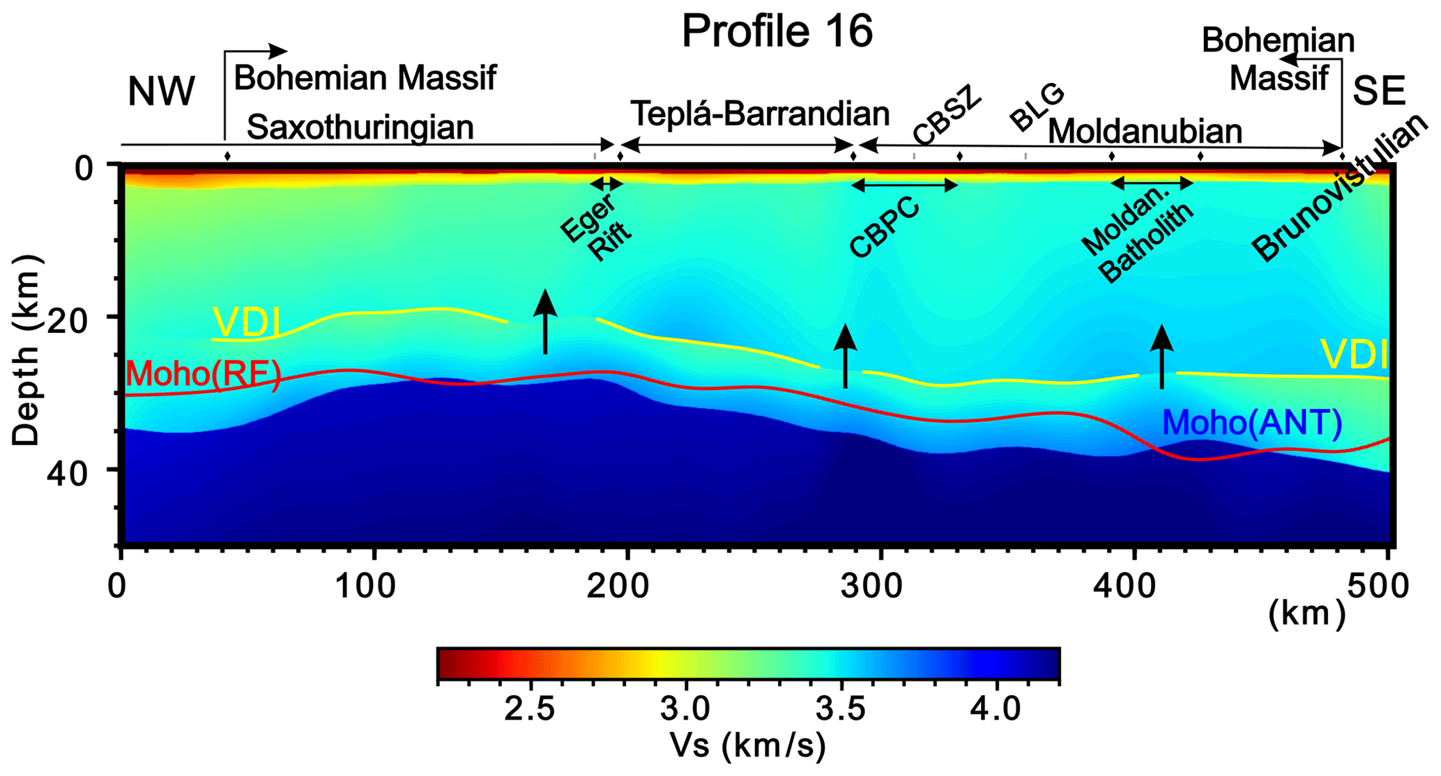
Figure 12A north-west–south-east oriented cross section through the core of the BM (see Fig. 11 for the location of the cross section), across the north-east–south-west trend of the Variscan structures. Note the regions of increased vS in the lower crust beneath the VDI interruptions. These regions can mark pathways (arrows) developed along the deep Variscan suture zones and boundaries of the individual tectonic units of the crust. The pathways allowed magma to percolate and feed the granitoid massifs (Central Bohemian Plutonic Complex and Moldanubian Batholith). The Moho depth, estimated from the Ps–P delay times in receiver functions calculated in this study, for all of the stations is shown in red. The vertical scale of the cross sections is exaggerated at 3:1.
Assuming a mafic composition (amphibolite-facie metamorphic rocks), a ductile flow in the lower crust is probably controlled by the deformation of plagioclase feldspar. The tendency of the lower crust to flow (e.g. Hacker et al., 2015) is controlled by its rheology. The onset of plagioclase viscous behaviour corresponds to a temperature of ∼450 ∘C (Cole et al., 2007). Based on heat-flow measurements in western Bohemia (Šafanda et al., 2007), such temperature can be reached at depths of around 20 km. Of course, the present-day depth of the top of the ductile lower crust, which shallows up to ∼15 km in some places, was modified by denudation that is estimated at about 7 km in the western BM (de Wall et al., 2019). On the other hand, the top of the lower crust deepens to ∼28 km (Fig. 8) in the south-eastern part of the BM core, which probably reflects thickening of the crust by Variscan (first oceanic, later continental) subductions (Medaris et al., 2006; Finger et al., 2007). Consequently, a thermal gradient was lowered due to the subductions of cold materials and by the time elapsed since these events took place; thus, the onset of ductile flow might have been deeper in the geological past.
Decoupling between the upper and lower crust due to rheological contrast between the two thermally different levels was suggested in the French Pyrenees (Denele et al., 2009). A similar model of mechanical decoupling between the brittle upper crust and a “hot deeper crustal level” is used to explain the crustal shortening during the India–Asia collision (Van Buer et al., 2015). Many seismic and magneto-telluric experiments within Tibet provide data that require models characterised by a less viscous mid-lower crust between a more viscous upper-crust and mantle lithosphere (e.g. Klemperer, 2006). Such interpretations agree with the widely accepted “jelly sandwich” model of Burov and Watts (2006) that can best explain the gross structural styles of plate tectonic collisional systems and also a large-scale flexure of the India Plate during the collision (e.g. Hetényi et al., 2006).
6.2.3 Regional distribution of the VDI and late-Variscan strike-slip tectonics
Most of the BM crust and its southern and western surroundings are characterised by the abrupt shear velocity decrease in the lower crust exceeding −0.4 km s−1 in some places (Fig. 8). Although the amplitude of the velocity drop and depth of the drop can be clustered according to individual tectonic units, there is only a weak relation between the depth of the VDI or the thickness of the LPC layer and the crustal thickness. The thickness of the imaged low-velocity layer varies from 8 to 13 km. The shallowest VDI (green in Fig. 8) is mostly mapped in regions with thinner crust (Fig. 6). On the other hand, the most significant velocity drop appears in both regions with thin and thick crust.
The VDI horizon, marked at sites where the velocity difference reaches at least −0.1 km s−1, is interrupted in several zones where the negative vS drop does not reach such a value or is absent. Evidently, such zones also appear as regions with no difference between the upper- and lower-crust velocities (Fig. 8) and often with a local velocity increase in the lowermost crust.
Figure 12 depicts a north-west–south-east cross section through the core of the BM, showing the vS in the crust of the four major tectonic units, which are former microplates assembled during the Variscan orogeny. The horizon of the VDI is interrupted above the mantle sutures and near the boundaries of crustal units, often laterally shifted from their mantle counterparts. The sutures probably served as subduction channels that later became paths along which subducted rocks were brought to the upper crust and provided magma for large granitoid massifs like the Central Bohemian Plutonic Complex or the Moldanubian Batholith (Babuška and Plomerová, 2013). The interruption of the VDI and relatively increased velocities in the lower crust also correlate with the deep sutures on other cross sections (Fig. 11b, c). No VDI interruption within the BM occurs along the S04 (Fig. 11a), which runs parallel to the EFZ and does not cross any distinct suture. This feature supports the importance of the late-Variscan strike-slip tectonics, in which the Elbe shear system played important role (Elter et al., 2020).
Contraction of the eastern Variscides caused by the north-westward advance of Gondwana resulted in a collisional shortening of the BM (Franke et al., 2017). The contraction was compensated for by late-Variscan strike-slip zones that considerably modified an original assembly of the BM (Pitra et al., 1999). Field measurements by these authors document dextral strike-slip movements along the Central Bohemian Shear Zone. This is in agreement with the model of the westward movement of a part of the TB lithosphere along the west-south-west oriented sutures on both sides of the TB unit (Babuška and Plomerová, 2017).
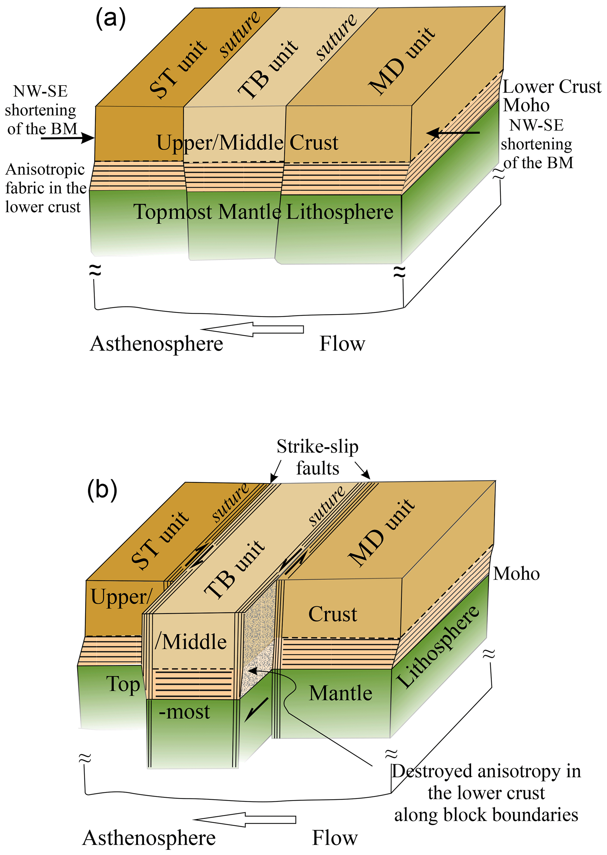
Figure 13Scheme of tectonic processes affecting the lower-crust fabric. (a) Bottom-driven north-west–south-east shortening of the core of the BM produced or enhanced pre-existing sub-horizontal foliation (fabric) within the lower-crust rocks. (b) Late-Variscan strike-slip fault systems often developed along the pre-existing deep sutures cutting the whole lithosphere. Movement along the sutures might locally modify, overprint, or erase the sub-horizontal fabric of the BM lower crust.
The model that we present in Fig. 13 can explain the spatial distribution of the VDI: why it is interrupted in places where the velocity decrease is weaker than −0.1 km s−1 or is absent. Most of the interruptions correlate with the deep boundaries of the tectonic units, e.g. ST–TB, TB–MD, and MD–BV (Babuška and Plomerová, 2013). Late-Variscan strike-slip movements preferably took place along such boundaries and most likely modified the sub-horizontal fabric of the lower crust by a system of parallel, deep-reaching faults. Strike-slip zones, like the CBSZ or the suture between the ST and TB units (see Fig. 12), undoubtedly cut the whole crust by sub-vertical faults that continue towards the mantle lithosphere. Movements along these zones disrupted the horizontal fabric and the VTI in the lower crust. Fabrics around the block boundaries might be modified locally into a more complex symmetry (e.g. the orthorhombic symmetry with ”fast” horizontal axis oriented in direction of movement) or might be entirely overwritten.
We present the first high-resolution 3-D shear velocity model of the entire Bohemian Massif crust and a map of Moho depths retrieved from ambient noise tomography. The model is based on recordings of more than 400 stations operated in several passive seismic experiments organised during the last 2 decades, including the large-scale AlpArray network (Hetényi et al., 2018a). The shear velocities modelled from dispersion curves of Rayleigh waves are ∼0.2 km s−1 higher in the BM upper crust than in its surroundings, with the highest velocities in the Moldanubian part. The region north of the Elbe Fault Zone exhibits relatively lower velocities. The presented 3-D model provides compelling evidence for regional-scale velocity variations in the Bohemian Massif.
Throughout the region, the Moho in the ambient noise tomography appears as a sharp interface, across which the lower-crust velocities (∼3.5–3.7 km s−1) attain the upper-mantle velocities (∼4.2 km s−1). The Moho shallows up to ∼28 km beneath the Eger Rift and its crossing with the Elbe Fault Zone. The Moho deepens down to ∼40 km in the Moldanubian part of the BM. In general, the Cadomian part of the region has a thinner crust, whereas the crust assembled, or tectonically transformed in the Variscan period, is thicker. The Moho discontinuity, as the dynamic phenomenon, retains remnants of Variscan subductions imprinted in bands of local crustal thickening.
The dominant feature of the presented 3-D velocity model is a relatively low vS in the lower crust that is in contradiction with the high vP modelled in the BM by the controlled source seismic profiles. We explain this seeming disagreement by the anisotropic structure of the lower crust, which is characterised by a transversely isotropic medium with a vertical “low-velocity” symmetry axis. We estimate the strength of anisotropy to be 3 %–9 % depending on the average vS. Considering the observed anisotropy and both the vP and vS interpreted from different field seismic experiments, amphibolite is the best candidate for the composition of the BM lower crust.
Due to the high density of data, thorough processing, and the enhanced depth sensitivity of the trans-dimensional tomographic inversion owing to layer stripping, layer averaging, and allowing for a velocity decrease with depth during the stochastic inversion, we were able to retrieve, for the first time, a distinct intra-crustal interface (VDI) with a velocity decrease as strong as −0.4 km s−1 in the lower part of the crust at depths of 18–30 km. In particular, the averaging of the best-fitting models over layers, instead of the commonly used averaging over fixed depth, proved to be crucial for the detection of velocity interfaces.
The VDI is interrupted around the boundaries of the crustal units, usually above locally increased velocities in the lowermost crust. Boundaries of the tectonic units likely served as subduction channels and partly as strike-slip zones in late-Variscan tectonic processes. Such zones can represent channels through which the high-velocity mantle material intruded into the lower crust. Portions of subducted and later molten crustal rocks percolated upwards providing magma to subsequently form granitoid massifs like the Central Bohemian Plutonic Complex and the Moldanubian Batholith. Moreover, the late-Variscan strike-slip movements rejuvenated such boundaries. These movements might have modified or erased the fabric of the lower crust and also interrupted the VDI horizon locally. This horizon and the lower-crust anisotropy probably reflect a rheological contrast between the formerly more viscous upper crust and less viscous lower crust.
The presented 3-D shear velocity model is homogeneous throughout the massif with unprecedented resolution. It tracks the variations in the velocities and the Moho depth at a grid of 0.2∘ N–S by 0.3∘ E–W. Understanding anisotropy in the lower crust can be further improved by the joint inversion of Rayleigh and Love waves, along with the receiver functions. The presented model is potentially of a great use in other geophysical studies and modern geological, petrological, and geochemical interpretations.
The final SV velocity model of the BM crust (CRAB1.0, Kvapil and Plomerová, 2021) is available at https://www.ig.cas.cz/en/teams/seismology/lithosphere-team/#crab1.0.
The supplement related to this article is available online at: https://doi.org/10.5194/se-12-1051-2021-supplement.
The complete member list of the AlpArray Working Group can be found at http://www.alparray.ethz.ch (last access: 1 May 2021).
JK collected the ambient noise data, carried out the data processing, and designed the methodology with contributions from JP, who interpreted the results, acquired funding, and supervised the research. VB contributed to geology interpretations, HKE computed receiver functions, and GH participated in the discussions. The paper was written by JP, JK, and VB with contributions from GH.
The authors declare that they have no conflict of interest.
This article is part of the special issue “New insights into the tectonic evolution of the Alps and the adjacent orogens”. It is not associated with a conference.
Research within this study was supported by the Grant Agency of the Czech Republic (grant no. 21-25710) and the CzechGeo/EPOS-Sci CZ.02.1.01/0.0/0.0/16_013/0001800 (OP RDE), CzechGeo/EPOS LM2010008, and LM2015079 projects. We acknowledge the operation of the XT temporary seismic network of the AlpArray-EASI complementary experiment (Hetényi et al., 2018a) and the AlpArray Seismic Network Z3 (2015) as well as several previous regional experiments in the Bohemian Massif. Special thanks go to Luděk Vecsey for his thorough data quality control. The authors are also particularly grateful to the AlpArray Seismic Network team, including György Hetényi, Rafael Abreu, Ivo Allegretti, Maria-Theresia Apoloner, Coralie Aubert, Simon Besançon, Maxime Bès De Berc, Götz Bokelmann, Didier Brunel, Marco Capello, Martina Čarman, Adriano Cavaliere, Jérôme Chèze, Claudio Chiarabba, John Clinton, Glenn Cougoulat, Wayne C. Crawford, Luigia Cristiano, Tibor Czifra, Ezio D'Alema, Stefania Danesi, Romuald Daniel, Anke Dannowski, Iva Dasović, Anne Deschamps, Jean-Xavier Dessa, Cécile Doubre, Sven Egdorf, Ethz-Sed Electronics Lab, Tomislav Fiket, Kasper Fischer, Wolfgang Friederich, Florian Fuchs, Sigward Funke, Domenico Giardini, Aladino Govoni, Zoltán Gráczer, Gidera Gröschl, Stefan Heimers, Ben Heit, Davorka Herak, Marijan Herak, Johann Huber, Dejan Jarić, Petr Jedlička, Yan Jia, Hélène Jund, Edi Kissling, Stefan Klingen, Bernhard Klotz, Petr Kolínský, Heidrun Kopp, Michael Korn, Josef Kotek, Lothar Kühne, Krešo Kuk, Dietrich Lange, Jürgen Loos, Sara Lovati, Deny Malengros, Lucia Margheriti, Christophe Maron, Xavier Martin, Marco Massa, Francesco Mazzarini, Thomas Meier, Laurent Métral, Irene Molinari, Milena Moretti, Anna Nardi, Jurij Pahor, Anne Paul, Catherine Péquegnat, Daniel Petersen, Damiano Pesaresi, Davide Piccinini, Claudia Piromallo, Thomas Plenefisch, Jaroslava Plomerová, Silvia Pondrelli, Snježan Prevolnik, Roman Racine, Marc Régnier, Miriam Reiss, Joachim Ritter, Georg Rümpker, Simone Salimbeni, Marco Santulin, Werner Scherer, Sven Schippkus, Detlef Schulte-Kortnack, Vesna Šipka, Stefano Solarino, Daniele Spallarossa, Kathrin Spieker, Josip Stipčević, Angelo Strollo, Bálint Süle, Gyöngyvér Szanyi, Eszter Szücs, Christine Thomas, Martin Thorwart, Frederik Tilmann, Stefan Ueding, Massimiliano Vallocchia, Luděk Vecsey, René Voigt, Joachim Wassermann, Zoltán Wéber, Christian Weidle, Viktor Wesztergom, Gauthier Weyland, Stefan Wiemer, Felix Wolf, David Wolyniec, Thomas Zieke, Mladen Živčić, and Helena Žlebčíková. Furthermore, we would like to thank all of the network operators providing data to the EIDA archive (http://www.orfeus-eu.org/eida, last access: 1 May 2021). The authors wish to acknowledge the creators of the software packages that we used for data processing and the creation of graphics: ObsPy (Beyreuther et al., 2010), MSNoise (Lecocq et al., 2014), FMST (Rawlinson, 2005), Geopsy (Wathelet et al., 2020), Python Matplotlib (Hunter, 2007), and GMT (Wessel and Smith, 1991).
This paper was edited by Emanuel Kästle and reviewed by Mariusz Majdanski and Amr El-Sharkawy.
Ackermann, L., Bizimis, M., Haluzová, E., Sláma, J., Svojtka, M., Hirajima, T., and Erban, V.: Re-Os and Lu-Hf isotopic constraints on the formation and age of mantle pyroxenites from the Bohemian Massif, Lithos 256/257, 197–210, 2016.
Almqvist, B. S. G. and Mainprice, D.: Seismic properties and anisotropy of the continental crust: Predictions based on mineral texture and rock microstructure, Rev. Geophys, 55, 367–433, https://doi.org/10.1002/2016RG000552, 2017.
AlpArray Seismic Network: AlpArray Seismic Network (AASN) temporary component, AlpArray Working Group, Other/Seismic Network, https://doi.org/10.12686/alparray/z3_2015, 2015.
Amaru, M.: Global travel time tomography with 3-D reference models, Geol. Traiectina, 274, PhD thesis, Utrecht University, The Netherlands, 174 pp., 2007.
Artemieva, I. and Thybo, H.: EUNAseis: A seismic model for Moho and crustal structure in Europe, Greenland, and the North Atlantic region, Tectonophysics, 609, 97–153, https://doi.org/10.1016/j.tecto.2013.08.004, 2013.
Babuška, V. and Plomerová, J.: Boundaries of mantle-lithosphere domains in the Bohemian Massif as extinct exhumation channels for high-pressure rocks, Gondwana Res., 23, 973–987, 2013.
Babuška, V. and Plomerová, J.: Lateral displacement of crustal units relative to underlying mantle-lithosphere: example from the Bohemian Massif, Massif as extinct exhumation channels for high-pressure rocks, Gondwana Res., 52, 125–138, 2017.
Bensen, G. D., Ritzwoller, M. H., Barmin, M. P., Levshin, A. L., Lin, F., Moschetti, M. P., Shapiro, N. M., and Yang, Y.: Processing seismic ambient noise data to obtain reliable broad-band surface wave dispersion measurements, Geophys. J. Int., 169, 1239–1260, https://doi.org/10.1111/j.1365-246X.2007.03374.x, 2007.
Beránek, B., Dudek, A., and Zounková, M.: Velocity models of the crust in the Bohemian Massif and the Western Carpathians (Rychlostní modely stavby zemské kůry v Českém masívu a Západních Karpatech), J. Geol. Sci. Appl. Geophys. (Sborník geologických věd, Užitá Geofyzika), 13, 7–17, 1975 (in Czech).
Beyreuther, M., Barsch, R., Krischer, L., Megies, T, Behr, Y., and Wassermann, J.: ObsPy: A Python Toolbox for Seismology, Seismol. Res. Lett., 81, 530–533, https://doi.org/10.1785/gssrl.81.3.530, 2010.
Bues, C., Dörr,W., Fiala, J., Vejnar, Z., and Zulauf, G.: Emplacement depths and radiometric ages of Paleozoic plutons of the Neukirchen–Kdyne Massif: differential uplift and exhumation of Cadomian basement due to Carboniferous orogenic collapse (Bohemian Massif), Tectonophysics, 352, 225–243, 2002.
Brückl, E., Blebinhaus, F., Gosar, A., Grad, M., Guterch, A., Hrubcová, P., Keller, G., Majdański, M., Šumanovac, F., Tiira, T., Yliniemi, J., Hegedüs, E., and Thybo, H.: Crustal structure due collisional and escape tectonics in the eastern Alps region based on profiles Alp01 and Alp02 from the Alp 2002 seismic experiment, J. Geophys. Res., 112, B06308, https://doi.org/10.1029/2006JB004687, 2007.
Burov, E. B. and Watts, A. B.: The long-term strength of continental lithosphere: “jelly sandwich” or “creme brulee”?, GSA Today, 16, 4–10, https://doi.org/10.1130/1052-5173(2006)016<4:tltSOc>2.0.cO;2, 2006.
Carbonell, R., Levander, A., and Kind, R.: The Mohorovičić discontinuity beneath the continental crust: An overview of seismic constraints, Tectonophysics 609, 353–376, 2013.
Červený, V., Novotný, O., Plešinger, A., and Plomerová, J.: Structure of the Earth's crust in southwestern Bohemia from spectral ratios of long-period P waves (preliminary results), Travaux Inst. Geophys. Tchecosl. Acad. Sci., XXV, No. 482, Geofysikální sborník XXV (1977), Academia, Praha 1977, 113–129, 1977.
Cháb, J. and Žáček, V.: Metamorphism of the Teplá crystalline complex, KTB Report, vol. 94, pp. 33–37, Niedersächsisches Landesamt für Bodenforschung, Hannover, Germany, 1994.
Cole, J., Hacker, B., Ratschbacher, L., Dolan, J., Seward, G., Frost, E., and Frank, W.: Localized ductile shear below the seismogenic zone: Structural analysis of an exhumed strike-slip fault, Austrian Alps, J. Geophys. Res., 112, B12304, https://doi.org/10.1029/2007JB004975, 2007.
de Wall, H., Schaarschmidt, A., Kammlein, M., Gerald, G., Bestmann, M., and Scharfenberg, L.: Subsurface granites in the Franconian Basin as the source of enhanced geothermal gradients: a key study from gravity and thermal modeling of the Bayreuth Granite, Int. J. Earth Sci. 108, 1913–1936, 2019.
Denele, Y., Olivier, P., Gleizes, G., and Barbey, P.: Decoupling between the middle and upper crust during transpression-related lateral flow: Variscan evolution of the Aston gneissdome (Pyrenees, France), Tectonophysics, 477, 244–261, 2009.
Dunkin, J. W.: Computation of modal solutions in layered, elastic media at high frequencies, B. Seismol. Soc. Am., 55, 335–358, 1965.
Elter, F. M., Gaggero L., Mantovani, F., Pandeli E., and Costamagna, L.G.: The Atlas-East Variscan -Elbe shear system and its role in the formation of the pull-apart Late Palaeozoic basins, Int. J. Earth Sci., 109, 739–760, https://doi.org/10.1007/s00531-020-01830-y, 2020.
Fichtner, A. and Villasenor, A.: Crust and upper mantle of the western Mediterranean–Constraints from full-waveform inversion, Earth Planet. Sci. Lett., 428, 52–62, https://doi.org/10.1016/j.epsl.2015.07.038, 2015.
Finger, F., Gerdes, A., Janoušek, V., René, M., and Riegler, G.: Resolving the Variscan evolution of the Moldanubian sector of the Bohemian Massif: the significance of the Bavarian and the Moravo–Moldanubian tectonometamorphic phases, J. Geosci. 52, 9–28, 2007.
Franke, W., Cocks, L. R. M., and Torsvik, T. H.: The Paleozoic Variscan ocean revisited, Gondwana Res. 48, 257–284, 2017.
Grad, M., Guterch, A., Mazur, S., Keller, G. R., Špičák, A., Hrubcová, P., and Geissler, W. H.: Lithospheric structure of the Bohemian Massif and adjacent Variscan belt in central Europe based on profile S01 from the SUDETES 2003 experiment, J. Geophys. Res., 113, B10304, https://doi.org/10.1029/2007JB005497, 2008.
Hacker, B. R., Kelemen, P. B., and Behn, M. D.: Continetal lower crust, Annu. Rev. Earth Planet. Sci. 43, 167–205, 2015.
Heron, P. J., Pysklywec, R. N., and Stephenson, R.: Identifying mantle lithosphere inheritance in controlling intraplate orogenesis, J. Geophys. Res.-Earth, 121, 6966e6987. https://doi.org/10.1002/2016JB013460, 2016.
Hetényi, G., Cattin, R., Vergne, J., and Nábělek, J. L.: The effective elastic thickness of the India Plate from receiver function imaging, gravity anomalies and thermomechanical modelling, Geophys. J. Int. 167, 1106–1118, https://doi.org/10.1111/j.1365-246X.2006.03198.x, 2006.
Hetényi, G., Molinari, I., Clinton, J., Bokelmann, G., Bondár, I., Crawford, W. C., Dessa, J-X., Doubre, C., Friederich, W., Fuchs, F., Giardini, D., Gráczer, Z., Handy, M. R., Herak, M., Jia, Y., Kissling, E., Kopp, H., Korn, M., Margheriti, L., Meier, T., Mucciarelli, M., Paul, A., Pesaresi, D., Piromallo, C., Plenefisch, T., Plomerová, J., Ritter, J., Rümpker, G., Šipka, V., Spallarossa, D., Thomas, C., Tilmann, F., Wassermann, J., Weber, M., Wéber, Z., Wesztergom, V., Živčić, M., AlpArray Seismic Network Team, AlpArray OBS Cruise Crew, and AlpArray Working Group: The AlpArray Seismic Network: a large-scale European experiment to image the Alpine orogeny, Surv. Geophys, 39, 1009–1033, https://doi.org/10.1007/s10712-018-9472-4, 2018a.
Hetényi, G., Plomerová, J., Bianchi, I., Kampfová Exnerová, H., Bokelmann, G., Handy, M. R., Babuska, V., and AlpArray-EASI Working Group: From mountain summits to roots: Crustal structure of the Eastern Alps and Bohemian Massif along longitude 13.3∘ E, Tectonophysics, 744, 239–255, https://doi.org/10.1016/j.tecto.2018.07.001, 2018b.
Hrubcová, P., Środa, P., Špičák, A., Guterch, A., Grad, M., Keller, G. R., Brückl, E., and Thybo, H.: Crustal and uppermost mantle stucture of the Bohemian Massif based on CELEBRATION 2000 data, J. Geophys. Res., 110, B11305, https://doi.org/10.1029/2004JB003080, 2005.
Hrubcová, P. and Środa, P.: Crustal structure at the easternmost termination of the Variscan belt based on CELEBRATION 2000 and ALP 2002 data, Tectonophysics. 460, 55–75, https://doi.org/10.1016/j.tecto.2008.07.009, 2008.
Hrubcová, P., Środa, P., Grad, M., Geissler, W. H., Guterch, A., Vozár, J., Hegedüs, E., and Sudetes 2003 Working Group: From the Variscan to the Alpine Orogeny: crustal structure of the Bohemian Massif and the Western Carpathians in the light of the SUDETES 2003 seismic data, Geophys. J. Int., 183, 611–633, https://doi.org/10.1111/j.1365-246X.2010.04766.x, 2010.
Hunter, J. D: Matplotlib: A 2D Graphics Environment, Comput. Sci. Eng., 9, 90–95, https://doi.org/10.1109/MCSE.2007.55, 2007.
Ji, S., Shao, T., Michibayashi, K., Long, C., Wang, Q., Kondo, Y., Zhao, W., Wang, H., and Salisbury, M. H.: A new calibration of seismic velocities, anisotropy, fabrics, and elastic moduli of amphibole-rich rocks, J. Geophys. Res.-Earth, 118, 4699–4728, https://doi.org/10.1002/jgrb.50352, 2013.
Kästle, E. D., El-Sharkawy, A., Boschi, L., Meier, T., Rosenberg, C., Bellahsen, N., Cristiano, L., and Weidle, C.: Surface wave tomography of the alps using ambient-noise and earthquake phase velocity measurements, J. Geophys. Res., 123, 1770–1792, 2018.
Karousová, H., Plomerová, J., and Babuška, V.: A three-dimensional velocity model of the crust of the Bohemian Massif, Stud. Geophys. Geod., 56, 249–267, 2012.
Karousová, H., Plomerova, J., and Babuska, V.: Upper-mantle structure beneath the southern Bohemian Massif and its surroundings imaged by high-resolution tomography, Geophys. J. Int., 194, 1203–1215, https://doi.org/10.1093/gji/ggt159, 2013.
Kennett, B. and Engdahl, R.: Travel times for global earthquake location and phase identification, Geophys. J. Int., 105, 429–465, 1991.
Klemperer, S. L.: Crustal flow in Tibet: Geophysical evidence for the physical state of Tibetan lithosphere, and inferred patterns of active flow, Geological Society, London, Special Publications, 268, 39–70, https://doi.org/10.1144/GSL.SP.2006.268.01.03, 2006.
Kokoska, S. and Zwillinger, D.: CRC Standard Probability and Statistics Tables and Formulae, Student Edition, CRC Press LLC, Boca Raton, Florida, USA, https://doi.org/10.1201/b16923, 2000.
Konopásek, J., Schulmann, K., and Johan, V.: Eclogite-facies metamorphism at the eastern margin of the Bohemian Massif–subduction prior to continental underthrusting?, Eur. J. Mineral., 14, 701–713, 2002.
Konopásek, J., Anczkiewicz, R., Jeřábek, P., Corfu, F., and Žáčková, E.: Chronology of the Saxothuringian subduction in the West Sudetes (Bohemian Massif, Czech Republic and Poland), Journal of the Geological Society London, 176, 492–504, https://doi.org/10.1144/jgs2018-173, 2019.
Kvapil, J. and Plomerová, J.: CRAB1.0 – A regional-scale crustal model of Bohemian Massif at 0.2 ∘N × 0.3∘ E from ambient noise tomography, available at: https://www.ig.cas.cz/en/teams/seismology/lithosphere-team/#crab1.0, last access: 1 May 2021.
Lay, T. and Wallace, T. C. (Eds.): Modern Global Seismology, Academic Press, New York, 521 pp., ISBN 0-12-732870-X, 1995.
Lecocq, T., Corentin C., and Brenguier, F.: MSNoise, a Python Package for Monitoring Seismic Velocity Changes Using Ambient Seismic Noise, Seismol. Res. Lett., 85, 715–726, https://doi.org/10.1785/0220130073, 2014.
Levshin, A. L. and Ritzwoller, M. H.: Automated detection, extraction, and measurement of regional surface waves, Pure Appl. Geophys., 158, 1531–1545, 2001.
Lobkis, O. I. and Weaver, R. L.: On the emergence of the Green's function in the correlations of a diffuse field, J. Acoust. Soc. Am. 110, 3011–3017, https://doi.org/10.1121/1.1417528, 2001.
Lu, Y., Stehly, L., Paul, A., and AlpArray Working Group: High-resolution surface wave tomography of the European crust and uppermost mantle from ambient seismic noise, Geophys. J. Int., 214, 1136–1150, https://doi.org/10.1093/gji/ggy188, 2018.
Lu, Y., Stehly, L., Brossier, R., Paul, A., and AlpArray Working Group: Imaging Alpine crust using ambient noise wave-equation tomography, Geophys. J. Int., 222, 69–85, https://doi.org/10.1093/gji/ggaa145, 2020.
Luo, Y., Xu, Y., and Yang, Y.: Crustal radial anisotropy beneath the Dabie orogenic belt from ambient noise tomography, Geophys. J. Int., 195, 1149–1164, 2013.
Majdanski, M. and Polkowski, M.: The Uncertainty of 2D Models Along Wide Angle Seismic Profiles, Pure Appl. Geophys., 171, 2277–2287, https://doi.org/10.1007/s00024-014-0840-9, 2014.
Medaris, L. G., Beard, B. L., and Jelínek, E.: Mantle-derived, UHP garnet pyroxenite and eclogite in the Moldanubian Gföhl Nappe, Bohemian Massif: a geochemical review, new p–t determinations, and tectonic interpretation, Int. Geol. Rev. 48, 765–777, https://doi.org/10.2747/0020-6814.48.9.765, 2006.
Molinari, I., Obermann, A., Kissling, E., Hetényi, G., Boschi, L., and AlpArray-EASI working Group: 3D crustal structure of the Eastern Alpine region from ambient noise tomography, Results in Geophysical Sciences, 1–4, 100006, https://doi.org/10.1016/j.ringps.2020.100006, 2020.
Mooney, W. D., Prodehl, C., and Pavlenkova, N. I.: 54 – Seismic Velocity Structure of the Continental Lithosphere from Controlled Source Data, International Geophysics, 81, 887–910, https://doi.org/10.1016/S0074-6142(02)80261-3, 2002.
Okaya, D., Vel, S. S., Song, W. J., and Johnson, S. E.: Modification of crustal seismic anisotropy by geological structures (“structural geometric anisotropy”), Geosphere 15, 146–170, https://doi.org/10.1130/GES01655.1, 2018.
Phinney, R. A.: Structure of the Earth's crust from spectral behavior of long-period body waves, J. Geophys. Res. 69, 2997–3017, https://doi.org/10.1029/JZ069i014p02997, 1964.
Pitra, P., Burg, J. P., and Guiraud, M.: Late Variscan strike-slip tectonics between the Teplá-Barrandian and Moldanubian terranes (Czech Bohemian Massif): petrostructural evidence, J. Geol. Soc. London, 156, 1003–1020, 1999.
Plešinger, A. and Horálek, J.: Seismic broadband recording and data processing system FBV/DPS and its seismological application, J. Geophys., 42, 201–217, 1976.
Plomerová, J., Babuška, V., and Ruprechtová, L.: Velocities of seismic waves propagating through the Bohemian Massif from foci in Poland, Studia Geophys. et Geod., 28, 56–66, 1984.
Plomerová, J., Achauer, U., Babuška, V., Vecsey, L., and BOHEMA working group: Upper mantle beneath the Eger Rift (Central Europe): plume or asthenosphere upwelling?, Geophys. J. Int., 169, 675–682; https://doi.org/10.1111/j.1365-246X.2007.03361.x, 2007.
Plomerová, J., Vecsey, L., and Babuška, V.: Mapping seismic anisotropy of the lithospheric mantle beneath the northern and eastern Bohemian Massif (central Europe), Tectonophysics 564, 38–53, 2012.
Plomerová, J., Munzarová, H., Vecsey, L., Kissling, E., Achauer, U., and Babuška, V.: Cenozoic volcanism in the Bohemian Massif in the context of P- and S-velocity high-resolution teleseismic tomography of the upper mantle, Geochem. Geophys. Geosyst., 17, 3326–3349, https://doi.org/10.1002/2016GC006318, 2016.
Qiao, L., Yao, H., Lai, Y-C., Huang, B.-S., and Zhang, P.: Crustal structure of southwest China and northern Vietnam from ambient noise tomography: Implication for the large-scale material transport model in SE Tibet, Tectonics, 37, 1492–1506, https://doi.org/10.1029/2018TC004957, 2018.
Qorbani, E., Zigone, D., Handy, M. R., Bokelmann, G., and AlpArray-EASI working group: Crustal structures beneath the Eastern and Southern Alps from ambient noise tomography, Solid Earth, 11, 1947–1968, https://doi.org/10.5194/se-11-1947-2020, 2020.
Rawlinson, N. and Sambridge M.: The fast marching method: An effective tool for tomographic imaging and tracking multiple phases in complex layered media, Explor. Geophys., 36, 341–350, 2005.
Rawlinson, N.: FMST: fast marching surface tomography package, Research School of Earth Sciences, Australian National University, Canberra, available at: http://rses.anu.edu.au/~nick/surftomo.html (last access: 1 May 2021), 2005.
Ren, Y., Grecu, B., Stuart, G., Houseman, G., Hegedüs, E., and South Carpathian Project Working Group: Crustal structure of the Carpathian–Pannonian region from ambient noise tomography, Geophys. J. Int., 195, 1351–1369, https://doi.org/10.1093/gji/ggt316, 2013.
Šafanda, J., Dědeček, P., Krešl, M., and Čermák, V.: Report on the geothermic research drill hole (Litoměřice) (in Czech), Geophysical Institute, Acad. Sci. of the Czech Rep, Praha, 2007.
Sambridge, M.: Geophysical inversion with a neighbourhood algorithm: I. Searching a parameter space, Geophys. J. Int., 138, 479–494, 1999.
Shapiro, N. M. and Campillo, M.: Emergence of broadband Rayleigh waves from correlations of the ambient seismic noise, Geophys. Res. Lett., 31, L07614, https://doi.org/10.1029/2004GL019491, 2004.
Shapiro, N. M., Campillo, M., Stehly, L., and Ritzwoller, M. H.: High resolution surface wave tomography from ambient seismic noise, Science, 307, 1615–1618, 2005.
Schippkus, S., Zigone, D., Bokelmann, G., and AlpArray Working Group: Ambient-noise tomography of the wider Vienna Basin region, Geophys. J. Int., 215, 102–117, https://doi.org/10.1093/gji/ggy259, 2018.
Soergel, D., Pedersen, H., Stehly, L., Margerin, L., Paul, A., and AlpArray Working Group: Coda-Q in the 2.5–20 s period band from seismic noise: application to the greater Alpine area, Geophys. J. Int., 220, 202–217, https://doi.org/10.1093/gji/ggz443, 2020.
Thybo, H., Artemieva, L. M., and Kennett, B.: Moho: 100 years after Andria Mohorovičić, Tectonophysics 609, 1–8, 2013.
Van Buer, N. J., Jagoutz, O., Upadhyay, R., and Guillong, M.: Mid-crustal detachment beneath western Tibet exhumed where conjugate Karakoram and Longmu-Gozha Co faults intersect, Earth Planet. Sci. Lett. 413, 144–157, 2015.
Valentová, L., Gallovič, F., and Maierová, P.: Three-dimensional S-wave velocity model of the Bohemian Massif from Bayesian ambient noise tomography, Tectonophysics, 717, 484–498, https://doi.org/10.1016/j.tecto.2017.08.033, 2017.
Wathelet, M., Jongmans, D., and Ohrnberger, M.: Surface wave inversion using a direct search algorithm and its application to ambient vibration measurements, Near Surf. Geophys. 2, 211–221, 2004.
Wathelet, M.: An improved. neighborhood algorithm: parameter conditions and dynamic scaling, Geophys. Res. Lett., 35, L09301, https://doi.org/10.1029/2008GL033256, 2008.
Wathelet, M., Chatelain, J-L., Cornou, C., Di Giulio, G., Guillier, B., Ohrnberger, M., and Savvaidis, A.: Geopsy: A User-Friendly Open-Source Tool Set for Ambient Vibration Processing, Seismol. Res. Lett., 91, 1878–1889, https://doi.org/10.1785/0220190360, 2020.
Wessel, P. and Smith, W. H. F.: Free software helps map and display data, EOS Trans. AGU, 72, 445–446, https://doi.org/10.1029/90EO00319, 1991.
Wilde-Piórko, M., Geissler, W. H., Plomerová, J., and PASSEQ Working Group: PASSEQ 2006-2008: passive seismic experiment in Trans-European Suture Zone, Stud. Geophys. Geod., 52, 439–448, 2008.
Yang, Z., Ritzwoller, M. H., Levshin, A. L., and Shapiro, N. M.: Ambient noise Rayleigh wave tomography across Europe, Geophys. J. Int., 168, 259–274, https://doi.org/10.1111/j.1365-246X.2006.03203.x, 2007.
Yoshizawa, K. and Kennett, B. L. N.: Sensitivity kernels for finite-frequency surface waves, Geophys. J. Int., 162, 910–926, https://doi.org/10.1111/j.1365-246X.2005.02707.x, 2005
Žák, J., Verner, K., Janoušek, V., Holub, F., Kachlík, V., Finger, F., Hajná, J., Tomek, F., Vondrovic, L., and Trubač, J.: A plate-kinematic model for the assembly of the Bohemian Massif constrained by structural relationships around granitoid plutons, Geological Society, London, Special Publications, 405, 169–196, https://doi.org/10.1144/SP405.9, 2014.
Zhu, L. and Kanamori, H.: Moho depth variation in southern California from teleseismic receiver functions, J. Geophys. Res. 105, 2969–2980, 2000.