


Abstract
The main goal of this study is to determine the solar origin of four single shocks observed at the Lagrange point L1 and followed by storm sudden commencements (SSCs) during 2002. We look for associated coronal mass ejections (CMEs), starting from estimates of the transit time from Sun to Earth. For each CME, we investigate its association with a radio type II burst, an indicator of the presence of a shock wave. For three of the events, the type II burst is shown to propagate along the same, or a similar, direction as the fastest segment of the CME leading edge. We analyze for each event the role of the coronal environment in the CME development, the shock formation, and their propagation, to finally identify its complex evolution. The ballistic velocity of these shocks during their propagation from the corona to L1 is compared to the shock velocity at L1. Based on a detailed analysis of the shock propagation and possible interactions up to 30 solar radii, we find a coherent velocity evolution for each event, in particular for one event, the 2002 April 14 SSC, for which a previous study did not find a satisfactory CME source. For the other three events, we observe the formation of a white-light shock overlying the different sources associated with those events. The localization of the event sources over the poles, together with an origin of the shocks being due to encounters of CMEs, can explain why at L1 we observe only single shocks and not interplanetary CMEs.
Export citation and abstract BibTeX RIS
1. Introduction
It has been widely recognized that type II radio burst emissions are the most direct diagnostic of shock waves in the solar corona. When a radio emission associated with a shock is detected in the corona, the shock can be due either to a flare or to a coronal mass ejection (CME) (e.g., Vršnak et al. 2006; Vršnak & Cliver 2008). However, when both are present, it is difficult to discriminate between these two possibilities. One of the main reasons for this ambiguity is the temporal synchronization of the impulsive phase of the flare with the CME acceleration phase. One possible physical interpretation of the shock wave origin is a blast wave ignited by the pressure pulse of a flare or a piston-driven shock due to a CME (e.g., Wagner & MacQueen 1983; Vršnak & Lulic 2000; Magdalenić et al. 2008; Nindos et al. 2011). We shall return to a more detailed discussion in Section 3.
Magdalenić et al. (2010) analyzed five selected CME/flare events associated with a type II burst and with rather slow CMEs. They found that the type II burst velocity was more compatible with the flare evolution than with the CME kinematic. They concluded that, for four of these events, the shock wave was most probably flare-generated and that the type II burst was generated by the energy release of the flare rather than by the CME expansion.
A recent study (Bocchialini et al. 2018) gave us the opportunity to return to the question of the link between shock waves and CMEs. The central objective of that study was the analysis of the solar sources associated with storm sudden commencements (SSCs) observed in 2002. Three main categories of interplanetary events were identified at L1: (a) those associated with interplanetary CMEs (ICMEs) or magnetic clouds (MCs); (b) those associated with streaming or corotating interaction regions (S/CIRs), not associated with CMEs and not considered any longer in what follows); and (c) four events, which were associated with a single isolated shock, without ICMEs, MCs, or S/CIRs detected at their vicinity. The investigation on the relationship between the L1 events and the CMEs observed by the Large Angle and Spectroscopic Coronagraph (LASCO)/Solar and Heliospheric Observatory (SOHO) coronagraph (Brueckner et al. 1995) showed that L1 events were associated at the Sun with a single CME or with an event resulting from a complex CME–CME interaction. However, their radio characteristics were found to be distinct. For the majority of the events belonging to the first category (ICMEs and MCs), the associated radio signature was both a type II and a type IV burst. Conversely, for the single-shock category, (called shock-only in Bocchialini et al. 2018), the radio signature was a type II burst and also, for three of them, a microwave burst.
Herein we present a more detailed data analysis of these four shock events, based on optical, X-ray, radio, and white-light observations. The main goals of this study are: (a) to determine the origin of the shocks at the Sun: flare-generated shock, or CME-driven shock? (b) to follow the CME and shock wave evolution in the LASCO C2 and C3 coronagraph field of views, and (c) to confirm or find a plausible source for the shock at L1 by propagation considerations, knowing that for one of the events no reliable source was found in Bocchialini et al. (2018).
2. The Single Shocks at L1
Among the 32 interplanetary shocks observed at L1 in 2002 giving rise to SSCs at Earth, the four events studied here (listed in Table 1) are labeled as "shock-only" (in Bocchialini et al. 2018 study) or "single-shock" (in our study) events, with no identified structure after the shock itself, as mentioned above and as can be seen in Figure 1. We refer to each shock event with the date of the associated CME and radio emissions as in Bocchialini et al. (2018). The associations were performed using velocity comparisons. The left column of Figure 1 presents the interplanetary magnetic field (IMF) and solar wind data at L1, obtained by the Advanced Composition Explorer spacecraft (ACE; Chiu et al. 1998) for the single shock in relation with the May 27 event. The timing of the interplanetary shock is marked with a plain cyan line. The sudden increase of the IMF (panel (b)), simultaneously with the increase of the solar wind density (panel (d)), speed, and temperature (not shown), indicates the arrival of the fast-forward interplanetary shock wave. During the 32 hr following the shock, the IMF orientation is stable (panel (c)), no flux rope structure can be seen in the IMF (panel (a)), and the solar wind density remains high (panel (d)). These observations indicate that there is no ICME following the shock at L1 (Bocchialini et al. 2018). Plots in Figure 1 have been obtained thanks to the CDPP AMDA tool (http://amda.cdpp.eu/).
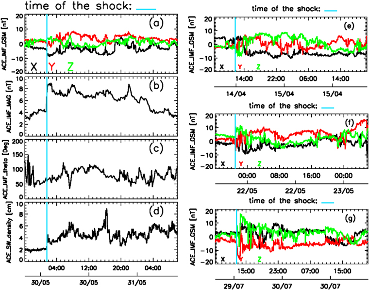
Figure 1. Observations at L1 of the four single-shock events by the Advanced Composition Explorer. Left panels (a)–(d) detail the observations of the interplanetary shock observed in association with solar event of May 27: three components of the interplanetary magnetic field (IMF), IMF magnitude, IMF inclination, and the solar wind density. The three IMF components of the three other shock events are plotted on the right panels (e)–(g) for respectively the April 11, May 17, and July 26 events. The vertical blue lines match the shock detection time at L1.
Download figure:
Standard image High-resolution imageTable 1. The Single-shock Events Associated with SSCs in 2002a
| SSC | L1 | Geoeffectiveness | |||
|---|---|---|---|---|---|
| Date | Time | B | Cat. | ΔV/V | Min(Dst) |
| (2002) | (UT) | (nT) | (nT) | ||
| Apr 14 | 12:34 | 10.1 | 0.6 | 1.1 | −23 |
| May 21 | 22:02 | 17.6 | 1 | 1.1 | −12 |
| May 30 | 02:04 | 9 | 0.6 | 1.2 | −13 |
| Jul 29 | 13:21 | 25.1 | 2 | 1.2 | 0 |
Note.
aThe first four columns give the date, time, amplitude (in nT), and category of the SSCs (see Table 1 of Bocchialini et al. 2018 for more explanation). The velocity jumps ΔV/V of the shocks observed at L1 are given in column 5. The last column gives the geoeffectiveness of the event, as defined by the Dst index minimum value observed after the SSC.Download table as: ASCIITypeset image
Single shocks related to the other three CME events (2002 April 11, May 18, and July 26) display similar features. The right column of Figure 1 (panels (e), (f), and (g)) gathers the IMF observed at L1 before and after these three interplanetary shocks. In panel (g) one can notice that the IMF intensification is first seen along the BY component, then along the BZ component, indicative of a quick IMF rotation. We also must notice that the induced SSCs are not intense. When looking at their characterization (see Table 1), only one is considered as a very clear event (index 2, SSC of July 29; see Table 1 of Bocchialini et al. 2018 for detailed explanations). Moreover, their amplitude is not very high, from 9 to 25 nT, being classified as 15, 21, 30, and 31 in order of decreasing intensity among the 32 SSCs recorded in 2002. While not a central point of the present study, let us mention their geoeffectiveness: their minimum Dst index values range between 0 and −23 nT, which is considered as not geoeffective (weak geomagnetic storm when min Dst > −30 nT). Those events had no noticeable effect on the Earth's thermosphere, contrary to the more intense events during the year 2002, for which shock waves were accompanied by MCs for instance.
In this study, we first identified the structure at Sun and/or in the solar corona whose consequence is a single shock at L1. We employed the hypothesis that the structure is faster than the ambient solar wind, which is justified as we will see later, and considered the possible link between both, verifying that the relation
is fulfilled. The VLASCO is the velocity of the structure at the edge of the field of view of the LASCO coronagraph, VBAL is the ballistic velocity between this point and L1, and VL1 is the velocity at L1 at the arrival of the shock.
3. Data Analysis
This section describes the analysis we performed to study the onset and development of each of these four events. Three events (April 11, May 18, July 26) which display a rather similar radio signature and evolution in the corona, are described in Section 3.3 and the last, more complex event, May 27, is described in Section 3.4.
For each of the studied events, a multi-panel figure gathers the main optical, X-ray, radio, and white-light observations.
3.1. Solar Data
The observations were obtained from various solar observatories and research groups.
- 1.Hα solar flares from Solar-Geophysical Data (NOAA), Holloman (New Mexico, USA (HOLL)), San Vito (Italy (SVTO)), Culgoora (Australia), Learmonth Observatory (Exmouth, WA, USA (LEAR)).
- 2.X-ray flares from the Geostationary Operational Environmental Satellite (GOES) and from the Reuven Ramaty High Energy Solar Spectroscopic Imager (RHESSI). Observations were provided by dedicated solar survey web sites at Dublin Trinity College (https://www.solarmonitor.org); Berkeley (http://sprg.ssl.berkeley.edu/~tohban/browser/).
- 3.Hα spectroheliograms from the Meudon survey (http://bass2000.obspm.fr/). Full-disk spectroheliograms in the Hα and CaH lines are also obtained for several wavelengths in each line.
- 4.MDI Magnetograms (Scherrer et al. 1995) and images from the Extreme Ultraviolet Imaging Telescope (EIT: Delaboudinière et al. 1995) from SOHO (Domingo et al. 1995) (see http://www.SolarMonitor.org).
- 5.Radio emissions from: (a) spectrograph observations: Nançay, France (DAM, 70–20 MHz), Tremsdorf, Germany (AIP, 80–40 MHz), Sagamore Hill, USA (SGMR, 80–30 MHz) and the WIND/Waves instrument onboard WIND (20 kHz–13.825 MHz, Bougeret et al. 1995); (b) discrete radio frequencies: Ondrejov, Czech Republic, and HIRAISO, Japan; (c) images at 164 MHz: Nançay Radioheliograph, France (NRH, 432–164 MHz; Kerdraon & Delouis 1997).
- 6.CME observations by LASCO C2 and C3 (Brueckner et al. 1995) onboard SOHO (see S0HO/LASCO CME catalog).
3.2. Shock Waves and Type II Burst Origin: Historical Context
The origin of the type II bursts in the solar corona remained for a long time a complex problem. Two possibilities were suggested and both of them were supported by some observations. One suggestion was that type II bursts in the low and middle corona (decametric–metric shocks) are temporally better associated with flares, which can initiate waves during their impulsive phase. The alternative scenario postulated that the corresponding coronal shocks are driven by mass motions such as ejecta, i.e., CMEs (see the review by Vršnak & Cliver 2008).
Although for some events observed at low frequencies (decametric–hectometric range), it was well established that the interplanetary type II burst shocks are directly driven by CMEs (e.g., Cane et al. 1987), the connection between these bursts and CMEs remained unclear at higher frequencies (metric range).
Maia et al. (2000) presented NRH imaging observations of weak metric type II radio bursts detected in the low corona which exhibited the properties expected for a CME-driven shock. They found excellent consistency in temporal and spatial progression between the type II radio sources and the front edge of the CMEs. The position of the radio-emitting source coincided with the CME leading edge. The authors concluded that these metric type II bursts were the counterpart of the hectometric and kilometric interplanetary type II bursts.
In agreement with numerous studies, the decimetric and metric type II bursts were found to originate in high-density structures, often a coronal streamer, situated close to the CME flank (e.g., Sheeley et al. 2000; Reiner et al. 2003; Cho et al. 2007). The streamers have a higher density, thus a lower Alfvén speed than the surrounding medium and this is considered as a favorable condition to generate type II bursts (e.g., Gopalswamy et al. 2005; Lin et al. 2006).
Moreover, it is today recognized that the shocks producing radio type II bursts can also result from (i) CME interactions with the ambient medium (e.g., Démoulin et al. 2012; Pick & Zhang 2012), (ii) CME–streamer interactions (e.g., Reiner et al. 2003; Cho et al. 2008; Feng et al. 2012; Magdalenić et al. 2014), and (iii) CME–CME interactions (e.g., Martinez Oliveros et al. 2012). More generally, Lugaz et al. (2017) presented a well-documented review of the different aspects, including the radio emissions, associated with the interaction of successive CMEs.
Vourlidas et al. (2003) showed in one event the signature of a fast magnetohydrodynamic wave propagating at the CME front and flanks, with a speed and density consistent with the existence of a fast-mode shock. This study was extended by Ontiveros & Vourlidas (2009) by selecting fast CMEs (>1500 km s−1). It confirmed that the large emission ahead and around the bright CME was the white-light counterpart of the CME-driven shock. It was also noted that all halo CMEs (10 events) have at least one location with such a shock signature, and this is consistent with a shock draping all around the CME-driven shock.
Yan et al. (2006) analyzed an event for which the CME development, the hard X-ray emission, and the type III burst group appear to be closely associated. Due to the development of the CME, this region becomes progressively highly compressed. Another signature of this compression region is a narrow white-light feature interpreted as a coronal shock driven by the CME lateral expansion. This result is in agreement with a more recent study regarding a CME-driven shock (Nindos et al. 2011).
Gopalswamy et al. (2007) studied the geoeffectiveness, speed, solar source, and flare association of a set of 378 halo CMEs of cycle 23 (1996–2005 inclusive). It was found that intense storms are generally due to disk halos and the few intense storms from limb halos occur only in the maximum and declining phases. More intense storms occur when there are successive CMEs. It was also found that the average speed of halo CMEs (corrected for projection effects) is more than double the average speed of the general population.
3.3. Data Analysis: 2002 April 11, May 18, July 26
In radio, at first glance, the onset of these three events looks rather similar. It is characterized by a microwave burst of short duration extending to lower frequencies, a signal which frequently marks the impulsive phase of a flare. The microwave burst is followed by a type II burst detected in the metric–decametric wavelength range and, for the July 26–27 event, also at kilometric wavelengths. Each of these events is associated with a CME observed in both the C2 and C3 field of views of the SOHO/LASCO experiment (see the associated details in Bocchialini et al. 2018).
3.3.1. 2002 April 11–12 Event
The April 11 event observations are given in Figure 2. The GOES C9.2 flare, associated with the 2002 April 11 event (panel (c)) was also detected by RHESSI (S15 W33 degrees, Active Region (AR) 9904). The corresponding active region is indicated by the right-hand white square on the EIT and MDI images (panels (a) and (b)). We note that AR 9904 seems to be magnetically connected with the nearby AR 9900 (marked with blue square in panel (b)). A microwave burst was observed at 16:20 by Ondrejov (2–4.5 GHz, panel (f)). Then a type II burst was observed by the Potsdam (80–40 MHz) and the Sagamore Hill (80–30 MHz) radio-spectrographs. Panel (d) displays the AIP dynamic spectrum showing the fundamental and the harmonic emission bands (marked by the white dashed line) of the type II burst. Note that, since the fundamental band is of low intensity, the type II speed was estimated from the harmonic band, assuming the 3× Saito model (Saito 1970), which gives the electron density as a function of the distance to the Sun—the radio emission being at the plasma frequency or at its harmonic. This is one of the most frequently employed 1D coronal electron density models for metric wavelengths. When radio emission is associated with a large flare and/or wide CME, the Saito density model is generally multiplied by a number larger than 1 (e.g., 2, 3, or 4) in order to account for denser ambient plasma conditions. Studies of several CME/flare events with sources situated close to the solar limb (Magdalenić et al. 2008, 2010) indicate that, for C-class and low M-class flares, the most appropriate coronal electron density profile to estimate the type II speed is about 3× Saito. The type II speed is found to be approximately 870 km s−1 (panel (l)). We can estimate the uncertainty in the velocity to be about 10%, resulting from this model. The change of the density profile from 4× to 2× Saito would induce, in this frequency range, a decrease in the type II speed of about 18% (Magdalenić et al. 2008).

Figure 2. April 11–12 event. Panels (a) Fe line (EIT), (b) MDI magnetogram, and (c) GOES X-ray measurements. Radio wave measurements: dynamic spectra from AIP (d) and Ondrejov observatories (f). SOHO/LASCO C2 images on top of which are EIT images (difference images: panels (e) and (h); direct image: panel (g)). SOHO/LASCO C3: difference images: panels (i) and (k); direct image: panel (j). Panels (l) and (m): time vs. height diagrams. For an explanation of the arrows, see the text.
Download figure:
Standard image High-resolution imageThe onset of the CME related to this flare is seen at about 16:50, and at 17:25 UT the CME is already well observed (panels (e) and (g)). The CME has a projected line-of-sight speed of 560 km s−1 (panel (l)). This speed was obtained by a linear fit to the height–time measurements in the SOHO/LASCO C2 field of view and was estimated in the direction of the fastest segment of the CME leading edge (PA, position angle = 242°). Panel (e) also shows signatures of the faint white-light shock, observed above the CME (marked with white arrows).
Propagation through the ambient medium. Kinematic curves in panels (l) and (m) give an indication that the CME and the type II burst are closely related, i.e., that type II is most probably associated with the CME-driven shock. One should note that there was a gap in the SOHO/LASCO observations between 16:26 and 16:50 UT. The type II burst is no longer observed by the AIP after 16:39 UT because it is out of its frequency range. The San Vito observatory also reports a type II burst in the range 172–28 MHz. However, WIND/Waves observations do not show continuation of the type II emission in the hectometer range and one possible explanation for this lack of radio emission is that the shock encounters the region of the local maximum of the Alfvén speed (Vršnak et al. 2004). Other possibility is that the continuation of the weak metric type II burst in the decameter to kilometer range, becoming even weaker, could not be observed, as its amplitude is below the instrument sensitivity.
At approximately 17:50 UT, the sudden onset of a new ejecta along the CME northern edge and underlying the streamer-like structure was observed. The ejecta was associated with the behind of the west limb flare, possibly originating from NOAA AR 9887 which rotated behind the limb on April 10. The ejecta is visible in panel (h), marked by black arrows, on EIT and LASCO C2. It is possible that the lateral part of the ejecta interacted with the CME. The CME front and the faint white-light shock continue their progression (see also white arrows, panels (i) and (k)). However, the white-light shock can no longer be clearly distinguished from the CME as a separate structure. On panels (e), (i), and (k) we observe, in addition to the white-light structure above the CME, a second discrete white-light region, shown by yellow arrows. This second white-light structure, which is weaker than the first one, is located above the streamer region close to the southern polar coronal hole (see CH on panel (a) and streamers on panel (j)). Its formation can be seen already starting from 17:26 UT (panel (e)). This white-light structure is possibly associated with eruptions from the complex region of NOAA AR 9896, 9898, and 9905. These three close regions (see the left-hand square on panels (a) and (b) in Figure 2 and the EIT movie at https://cdaw.gsfc.nasa.gov/CME_list/UNIVERSAL/2002_04/univ2002_04.html) were the source of flares and of numerous ejecta on April 11 and 12. The Nançay radiotelescope, which observed the Sun until 15:20 UT, showed the presence of successive radio bursts at 432 MHz, detected above the region 9905. This suggests that these regions are the sources of the ejecta. Some of the ejecta were indeed found to propagate along the streamer situated along the western edge of NOAA AR 9905 (marked with a pale blue arrow in panels (g) and (j)), reaching the streamer situated close to the southern polar coronal hole and then building-up the new region overlying this streamer (marked with yellow arrows in panels (e), (h), (i), and (k)). The majority of streamers (panel (j), pale blue and green arrows) originate from the same regions, essentially NOAA ARs 9905 and 9898. We note that the elongated white-light structure, which plays the role of a bridge linking the two sides (two separated yellow arrows in panel (k)) somewhat coincides with that of the CME observed earlier that day (e.g., LASCO C3 image at 05:18 UT on 2002 April 11).
The white-light structures enhanced by the two yellow arrows on panel (k) are linked to AR 9898 and 9905 which were very active throughout April 11 and persisted at least up to 10:42 UT on April 12 (see https://cdaw.gsfc.nasa.gov/CME_list/daily_movies/2002/04/12).
Our analysis suggests that the structure indicated by the two yellow arrows might be at the origin of the shock observed at L1. The two figures at 00:18 UT show the link between the streamers and the shock region as well as with the ejecta. This white-light structure propagates with a speed of 720–840 km s−1 (panel (m)).
In conclusion, Figure 2(k) shows that, at an altitude of about 30 solar radii, two distinctive but faint white-light structures are observed. The first one is observed above the western CME and the type II burst region (panels (i) and (k), white arrows) and the second one above the streamer region (panels (h), (i), and (k), yellow arrows). The white-light structure above the streamer region shows the extent (two separated yellow arrows in panel (k)) toward the other part of the white-light structure (marked with white arrows).
The two white-light structures (possibly shock waves) propagate further on more or less synchronously, suggesting that they might be part of one extended white-light structure. Nevertheless, it is difficult to conclude if these two structures, of clearly different origin, indeed interacted. We also note that, although these two shock regions are located near the edges of a coronal hole (Figure 2(a)), their evolutions remain quite independent.
Link with L1 observations. We first consider the CME (PA = 242) as a possible source of the shock observed at L1 on April 14. The corresponding ballistic velocity, VBAL, is 620 km s−1, the shock velocity at L1, VL1, is 420 km s−1, and the CME velocity at the Sun, VLASCO, is 560 km s−1. In this case, the relationship defined above, VLASCO > VBAL > VL1, is not fulfilled. This CME was already noted as somehow unsatisfactory in Bocchialini et al. (2018).
The shock overlying the streamer regions described above, whatever its exact origin, is the most satisfying candidate: its velocity (710–840 km s−1) is larger than the ballistic velocity and it is not directly related to an ICME. This latter property would explain the lack of a clear ICME signature at L1. There is no indication at L1 of fast solar wind usually related to coronal holes. The shock observed at L1 could result from the side of the shock-like white-light feature.
3.3.2. 2002 May 18 Event
The May 18 event observations are given in Figure 3. GOES (panel (c)) and SVTO observed two flares very close in position and in time (SVTO: S21 E38, 11:31–11:33–11:40 UT; S14 E36, 11:33–11:37–11:45 UT). The source region is shown on the EIT and MDI images (white squares on panels (a) and (b)). In association with these flares, a type II-like burst of short duration was observed in the decametric frequency range by the Nançay radio spectrograph (panel (e)) and occurred in temporal coincidence with a high-frequency burst observed by Ondrejov (panel (d)) and by the NRH at metric wavelengths (panel (f), red arrow). Similar to the previous event, WIND/Waves spectra show only weak type III bursts and no type II emission in the hectometer to kilometer wavelength range.

Figure 3. May 18 event; notation similar to Figure 2. Radio wave data: Ondrejov (d) and DAM/Nançay (e) dynamic spectra; NRH 3D image at 164 MHz (f).
Download figure:
Standard image High-resolution imageAs shown in the combined SOHO/LASCO/C2 and EIT image at 11:50 UT (panel (g)), we observe the emergence of a white-light structure which marks the onset of the CME. This structure progressively splits into two parts (CME1a and CME1b) as observed between 11:50 UT (panel (h)) and 12:06 (panel (i); see also red arrows). Panels (h) and (i) of Figure 3 show that CME1b becomes strongly elongated with a slightly changing inclination, and it propagates along a direction with a PA of about 165°. The progression of both CME 1a and CME 1b is shown in panel (n). On the same graph, one can also distinguish around 12:48 UT (marked with a vertical red line) CME1a, which displays a slightly different inclination. The main propagation direction of CME 1a is along PA = 148°, and its velocity is somewhat smaller than the speed of CME 1b. As hereafter discussed, CME1b encounters around 13:30 UT another CME (CME2; dark blue arrow in panel (j)). This, together with the possible projection effects, could explain why, in this event, the coronagraph observations do not show clear signatures of the white-light shock associated with CME1. We do not analyze in detail their kinematics due to the possibly ambiguous results.
Propagation through the ambient medium. At its western edge, the white-light ejecta CME1b (panel (i)) first interacts with the flanks of the neighboring faint CME (CME0 PA angle 194°, panel (h)). After 13:30 UT, the CME1b comes into contact with CME2 (dark blue arrows in panels (j) and (l); onset 13:27 UT, PA = 217°), which is observed in the southwest quadrant of the Sun. At about 14:18 UT (not shown), we start to observe an elongated white-light edge (looking like a shock) overlying CME1b and CME2, clearly visible at 14:42 UT (panel (k), yellow arrows). We also note the onset of a streamer blow out along the northern edge of CME2 (pale blue arrow in panels (j) and (m)). This ejection along the streamer changes progressively its orientation while it propagates away from the Sun (its speed is about 850 km s−1). The SOHO/LASCO/C3 images, at 17:18 (panel (l)) and 20:18 UT (panel (m)) show that the white-light shock and CME1b have reached the edge of the C3 field of view i.e., 30 Rs near 20:18 UT with a velocity estimated, at 26 Rs, to be about 500 km s−1 (consistent with the CME 1b velocity, see panel (n)). Figure 3, panels (k) and (l) clearly show that the white-light shock-like structure has developed and is overarching CME1b and CME2 (yellow arrows).
Link with L1 observations. The ballistic velocity that matches the interplanetary shock observation at L1 associated to that event is about 500 km s−1, and the observed velocity at L1 is about 400 km s−1. The leading shock of CME1b (up to 540 km s−1) is the most relevant to match shock observations at L1. The origin of this L1 shock results from the development of the shock-like structure apparently originating from CME2 and then overarching successively CME1b and also CME1a. A large part of the shock region is located above or close to the disk center and propagates along a direction very close to the Sun–Earth line. CME1b and the CME2 eastern flank are located at a larger distance from the Sun–Earth line. One concludes that the event observed at L1 will be an isolated shock.
3.3.3. July 26–27 Event
The July 26–27 event observations are presented in Figure 4. The GOES M5.3 flare associated with July 26–27 event (panel (c)), was detected in Hα by HOLL at position S19 E26 (20:51 21:13 22:59 UT, NOAA 10044). This AR is marked by a white square on the EIT and MDI images (panels (a) and (b)). This flare marks the onset of a series of radio bursts observed mainly at 500 MHz by HIRAISO (panel (d); green arrow). The C2 coronagraph image shows at 22:06 UT (panel (g)) the onset of the CME, which then displays a strong lateral expansion during the time interval 22:06–22:30 UT. The CME reaches a very narrow streamer at its western side (white arrows in panels (f) and (g)), at about 22:30 UT. The lateral expansion seems to be associated with a flare at about 22:05 UT (GOES 22:03 22:17 22:32 UT, panel (c)), as suggested by the radio observations from HIRAISO at 2 GHz and at lower frequencies, 500 MHz (see panel (d), respectively blue and black arrows). The observations suggest that a CME-driven shock interacts with the streamer, and this causes the type II burst observed by the WIND/Waves radio spectrograph during the 22:27–23:30 UT period in the 12–1 MHz frequency range (panel (e)). Applying the Leblanc electron density model (Leblanc et al. 1998), which describes well radio emission observed in the decameter to kilometer wavelength range, and type II drift rate, we estimated the type II burst and associated shock wave speed to be of the order of 620 km s−1 (panel (j)).
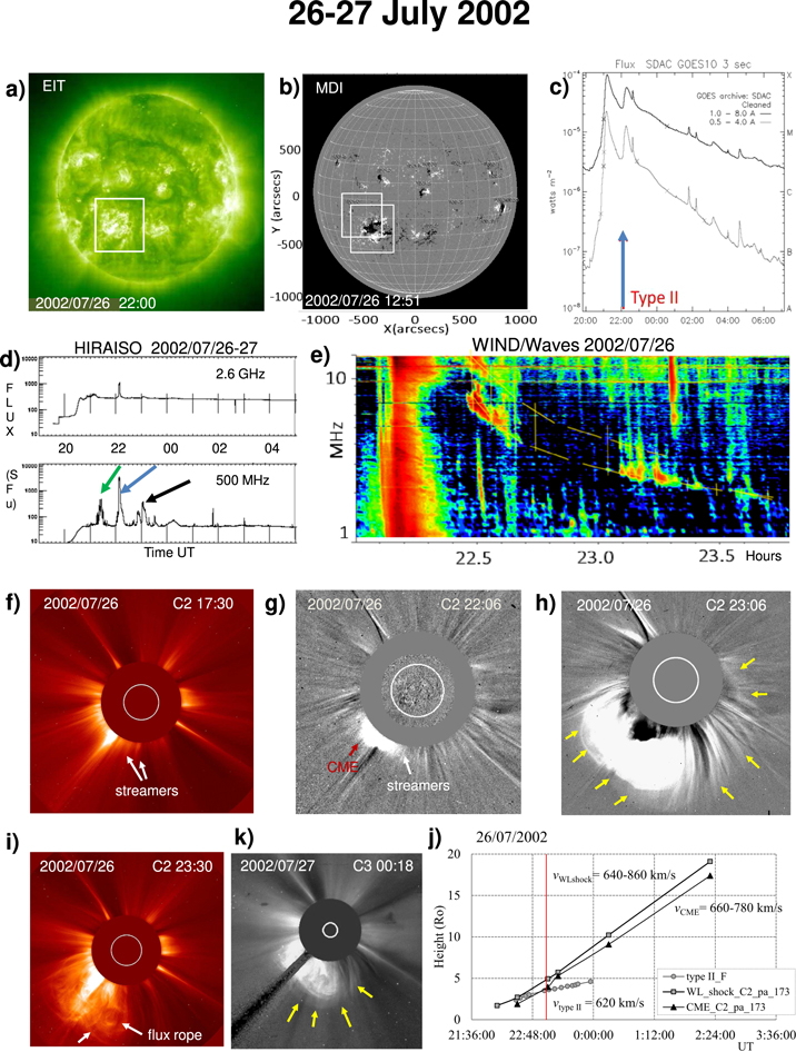
Figure 4. July 26–27 event; notation similar to Figure 2. Radio wave data: two frequency channels from HIRAISO (d); WIND/Waves radio spectrum (e).
Download figure:
Standard image High-resolution imageLet us note that this event is indicated in the SOHO/LASCO catalog as a halo CME.
Propagation through the ambient medium. The fact that the type II burst is being generated at the interface between the shock at the CME flank and the nearby streamer (see panel (f)) might explain the unusual crossing of the CME and the type II propagation curves visible on panel (j). However, we also need to keep in mind that the kinematics presented in panel (j) shows a projected CME and the shock wave propagation, and we do not know their exact 3D relationship. At first, shock signatures seem to be in front of the CME and, after the crossing, behind it. This behavior can be explained by the type II source region being close to the CME flank and not the leading edge. Similarly, interaction of the CME-driven shock and a streamer was found to be the reason for enhancement of the type II emission in the study by Magdalenić et al. (2014).
Associated with the flare observed by LEAR (23:31E:23:31U-26:00) which originated from the same NOAA AR10044 as the M5.3 flare, we observe the development of the flux rope along the streamer region (panels (i) and (k)). Similarly to the previous CME, the associated radio emission detected predominantly at 500 MHz (see panel (d), black arrow) and not on the dynamic spectra indicates the possible interaction between the CME-driven shock and the streamer.
The propagation direction of this flux rope differs only by a small angle (about 2°–3°) from the direction corresponding to the fastest segment of the CME leading edge (PA = 173°).
The SOHO/LASCO/C3 coronagraph image at 00:18 UT (panel (k)) shows that the flux rope and the CME front are in contact, and progress together surrounded by the white-light shock (marked by yellow arrows). They reach the 30 solar radii altitude approximately at 05:18 UT (not shown) with a maximum speed of about 780 km s−1 (CME front) and 860 km s−1 (white-light shock). This is consistent with the results presented in panel (j).
The lateral CME edge comes into contact with another region composed of a series of jets or jet-like structures (at about 05:18 UT). The first jet encounter leads to a clear distinction between these two regions propagating with different inclinations, both originating from the same halo CME and surrounded by the same white-light shock. Moreover, the direct image at 06:18:05 UT (not presented) shows that at that time the flux rope comes into contact with the jet-like structures (see Figure 6; this will be discussed below). This second event will propagate with a speed of about 700 km s−1 and will reach L1 as a driver-less shock. We note that, as we have only 2D images which suffer from the line-of-sight projection effects, we cannot fully exclude the possibility that the jet-like structures are just density enhancements of the CME structure.
Link with L1 observations. The ballistic velocity that matches the interplanetary shock observation at L1 associated with this event is about 650 km s−1, and the observed velocity of the shock at L1 is about 500 km s−1. The structure following that interplanetary shock looks like a sheath without a clear ICME. White-light shock velocities measured with LASCO, clearly larger than 650 km s−1, match the velocity criterion (VLASCO > VBAL > VL1).
3.4. Data Analysis: 2002 May 27
The origin at the Sun of the shock observed at L1 on May 30, 02:04 UT, was attributed to a partial halo CME (CMEP26; in Bocchialini et al. 2018). The CME was first seen in the SOHO/LASCO C2 field of view at 13:27 UT on 2002 May 27, straight after a data gap (from 12:50 to 13:27 UT). The CME width was about 160° and its projected line-of-sight speed was about 1200 km s−1. This CME was associated with a flare observed by GOES, by EIT (cadence 12 min), and by RHESSI (cadence 4 s) and it lasted from 12:23 UT until 13:25 UT.
May 27 event observations are presented in Figure 5. Panels (l)–(p) display SOHO/LASCO C2 and C3 difference images. In the first available image at 13:27 UT (panel (l)), the CME is already fully developed. Two bright and elongated ejecta (denoted as J1 and J2 in panels (l) and (n)) are also visible in all the C2 and C3 images.

Figure 5. May 27 event. Panels (a)–(d): active region in heliographic coordinates (x = (−460'', 0''), y = (200'', 600'')): (a) and (b): Hα images from the Meudon survey spectroheliograph, (c): MDI magnetograph, (d): EUV image from SOHO/EIT. Panel (e): 3 s resolution GOES X-ray flux. Radio wave data: east–west (f), (g) and north–south (f) NRH data at 164 MRH; NRH images (h), (j), (k) ; WIND/Waves dynamic spectrum (i). Panels (l)–(q): see Figure 2.
Download figure:
Standard image High-resolution image3.4.1. Solar Activity: Its Link with Eruptive Structures
During the time interval 12:25–13:25 UT, the NRH observed at 164 MHz two successive periods of radio emission (named Jr1 and Jr2), associated with J1 and J2 ejecta, respectively (Figure 5, panels (f), (g), (h), (j), and (k)). Both periods of radio emission were associated with the same AR and drifting in the eastern direction, with a distinct southward inclination (see panels (f) and (g)). The first period of radio emission (Jr1 in panel (f)) with an onset at about 12:25 UT, is associated with an X-ray flare C2.7 (12:23:52–12:29:40 UT) detected by EIT (panel (d)) and GOES (panel (e)) in the region located at N25 E10 (deg), i.e., in the same source region as for the CME at 12:23 UT. This episode lasts until about 12:37 UT (see panels (f) and (g)).
The onset of the radio emission (Jr2 in panel (f)) associated with J2 ejecta is at 12:36 UT. A radio source is detected until about 12:50 UT. Its development is much more complex than that of the first period Jr1, as we see from the panel (g). Jr2 includes three successive radio bursts: (a) at 12:36 UT (denoted XR-F), (b) at 12:51 UT (denoted XR-F II), a time at which is also detected a type II burst, and (c) at 13:08 UT (denoted XR-F). Each of these bursts was associated with an X-ray flare detected by RHESSI, as indicated in the (g) upper scale, and also by GOES (see Section 3.4.2). The three X-ray flares are indicated by red arrows in Figure 5, panel (e) (see also Section 3.4.2).
The NRH images (panels (h), (j), and (k)) obtained at the time of the X-ray flares show almost the same source position of the radio emission for all three instances. We can conclude that all the radio and X-ray flares appear to originate at approximately the same position, i.e., below the J2 ejecta (panel (l)).
3.4.2. Active Region and Flare Origin
Figure 5 (panels (a)–(d)) displays the Hα images from the Meudon survey spectroheliograph (a), (b) and the MDI magnetograph on board SOHO (c), as well as the EUV images from SOHO/EIT (d). Panel (e) shows that four flares were detected by GOES at 12:27 UT, 12:32–12:36 UT (two maxima), 12:54, and 13:13 UT. These events were detected in the region located at N25 E10 (see https://www.solarmonitor.org/?date=20020527) and were, except the first one (gray shadow in (e)), also detected in X-ray by RHESSI (see top of panel (g) and the three red arrows in panel (e)). On the top of panel (e), the time of observation of the successive X-ray flares is reported.
In the optical range, only two spectroheliograms are available: the first one, at 09:49 UT (panel (a)), shows a large, half round-shaped filament which erupted around 12:36 UT according to EIT observations (see the EIT movie). This filament eruption produces the J2 and Jr2 period event observed by the NRH (maximum 12:36 UT; panel (h)) and by GOES at 12:39 UT (panel (e)). Then, EIT observations show the development of the two-ribbons flare. The two ribbons, R1 and R2, are linked by flare loops (panel (b)). The reconnection along the magnetic inversion line is recurrent at 12:54 and 13:13 UT with two X-ray events of C-class. With RHESSI we can identify the projected location of the source at the polarity inversion line in the energy range 12–25 keV between 12:51 and 12:54 UT (middle of the oval symbol, reported in panel (c) at 12:48 UT). This is also the strongest event, during this period, observed in radio wavelengths by the NRH.
The lack of coronagraph observations between 12:13 and 13:27 UT makes it difficult to investigate the possible link between the CME and the two periods Jr1 and Jr2. As the first episode ends at 12:36 UT, we shall focus exclusively on the second one.
3.4.3. The CME Evolution
We can already distinguish J1 and J2 ejecta in the first available CME image (13:27 UT, panel (l)). On the two next available images at 13:50 UT (panel (m)) and 14:42 UT (panel (n)), J1 and J2 become clearly distinguishable. J1 and J2 follow two distinct trajectories. One should note that already at 14:42 UT, in the C3 image (panel (n)), a well-defined white-light shock wave overarching all the observed ejecta is detected (marked by yellow arrows).
One should note the presence of a streamer (see C2 13:27; panel (l), red arrow) situated apparently above the north pole region, and detected since 00:18 UT the same day, i.e., the first available image provided by SOHO on May 27. Bending of this streamer, well observed at 13:27, 13:50 and 14:42 UT (red arrows in panels (l)–(n)), is due to the passage of the shock wave associated with the CME. At the same time, the image on panel (n) shows two regions of enhanced density above J1 and J2, located along the CME. As already mentioned, we shall exclusively focus on the CME region located above and around J2. At 16:18 UT the region of enhanced density overlies the CME, and now extends toward the northern pole, the J2 position corresponding to its southward limit (panel (p)).
Running the difference image at 16:18 UT (panel (p)) shows that the CME progression in latitude is now constrained by J1 on its left-hand side and (blue arrow) on its right-hand side, by the streamer in the north polar region. One also observes the presence of another smaller ejecta, indicated by a white arrow in panels (o) and (p), propagating roughly above the north solar pole. Panel (q) displays the kinematic of the CME and the white-light shock (at two different position angles, PA = 34° and 9°, i.e., J2 region). The shock wave velocities at these different position angles are found to be the same and also comparable to the CME speed, 1160 km s−1 and 1090 km s−1 respectively.
These velocities are compatible with the calculated ballistic velocity (650 km s−1) and the measured velocity of the shock at its arrival at L1 (500 km s−1), assuming that the fast shock wave strongly decelerated during its travel through the ambient solar wind.
3.4.4. The Type II Burst and the Shock Wave
A type II burst, with an onset near 12:30 UT was detected by WIND/Waves (https://cdaw.gsfc.nasa.gov/CME_list/radio/waves_type2.html). The WIND/Waves observations show that this rather weak event was observed in the frequency range 14–5 MHz. We were able in fact to observe it in only the 8–3 MHz frequency range (see panel (i)) and to properly study three frequencies, 7.5, 5.4, and 3 MHz, at three different times. At those times, we estimated its altitude using, similar to event 3, the Leblanc coronal electron density model (Leblanc et al. 1998). We consider that the type II burst is the fundamental plasma emission, as is usually the case in this frequency range. A red cross in panel (l) (13:27 UT) indicates the approximate shock position measured at 3 MHz at 13:34 UT, assuming that the shock wave propagates along the same position angle as J2. Its velocity is estimated to be of the order of 1240 km s−1 (panel (q)). We note that the position of the type II radio burst is the projected one and it depends on the applied electron density model. This is probably why it does not fully coincide with the observed white-light shock.
4. Summary and Conclusion
The aim of this study is to investigate the solar origin and the evolution of the four events of 2002 associated at L1 with a single shock and then with an SSC, evidenced in Bocchialini et al. (2018).
Although these events shared, near their onset, some similar characteristics in the radio-frequency domain (a microwave burst followed by a type II radio emission and absence of type IV radio emission), each one displays its own complex history.
The onset phase. Three events (April 11, July 26, and May 18) are associated with a flare and a microwave burst, followed by the onset of a CME and a type II burst. For two of them the type II burst is clearly associated with a CME-driven shock wave and streamer interaction. For the third one (May 18), the type II burst duration was too short to allow us to unambiguously determine its velocity and association with the CME and nearby ambient coronal structures.
The type II burst observed on May 27 propagated in a direction similar to that of the fastest segment of the CME leading edge.
We conclude that, for three events, those for which we were able to estimate the velocity, the type II burst propagated along the same or a comparable direction to the fastest segment of the CME leading edge.
Propagation through the ambient medium. The data analysis that was performed for each event up to 30/32 Rs illustrates well the complexity of their travel in the corona and the variety of interactions which probably modified their propagation, and leads to an understanding of the origin of the shocks observed at L1. As only single-point observations are available for the studied events, it was not possible to quantify how much the shock wave and CME modify their propagation direction due to the complex interactions they go through.
A summary of the results obtained in this analysis is given in Figure 6. For each event a LASCO/C3 image shows the probable driver of the shock seen at L1 reaching 30 Rs, the shock direction, and the surrounding structures.

Figure 6. Summary of the four events. For each event, one image is shown giving the shock direction and highlighting the surrounding structures, when reaching 30 Rs.
Download figure:
Standard image High-resolution image
It is widely recognized that structures other than the CMEs might also be involved in geomagnetic activity, such as high-speed streams and shock disturbances (e.g., Gosling et al. 1991; Richardson et al. 2001; Webb 2002) as illustrated and briefly summarized for the four events.
- 1.2002 April 11–12. We observe two discrete shock regions, located at distinct longitudes, and which apparently follow their own propagation direction, but with a comparable velocity. If the two white-light structures are part of the same shock wave, their association with the in situ shock signatures is clear. Let us recall here that, whereas a CME associated with the ejection of a filament propagates in most cases at an almost constant speed in the interplanetary medium, CMEs associated with a flare, which is the case with this event, were more frequently found to decelerate during their propagation in the interplanetary medium (Andrews & Howard 2001; Vilmer et al. 2003). This is indeed what we observe in the present case, in particular for the second shock region observed at 30 Rs. Moreover, the orientation of the second event is more appropriate than that of the first event (see Figure 6). This event shows the development of a second branch which displays two regions, each one overlying a streamer and also an ejecta i.e., it presents the conditions which are favorable to the shock's development. This second branch of the white-light structure stretches towards a region close to the type II burst region.
- 2.2002 May 18. This event displays at the origin two CMEs, one in the eastward and one in the westward direction. A white-light structure (possibly a shock wave) is formed overarching the observed ejections.The shock observed at 30 Rs results from the combination of several components, all clearly oriented along a direction close to the Sun–Earth line (see Figure 3 panel (l), yellow arrows).
- 3.2002 July 26–27. The origin of the shock in this event essentially results from the lateral expansion of a halo CME which surrounds the whole Sun and in which one can distinguish two steps: (a) the first encounter with a streamer, followed by the build-up of a flux rope, which will later on enter in contact with the halo CME front; (b) the CME then continues its lateral progression and comes into contact with a new region composed of a series of jets having a distinct inclination. These two broad regions are surrounded by the same white-light shock. This second event will reach L1 as a driver-less shock.
- 4.2002 May 27. Data analysis had to be concentrated mainly on the north solar hemisphere, in which the same active region was the source, over two hours, of several X-ray flares, of one CME, three ejecta, and a type II burst. A part of the ejecta and the shock modified gradually their orientation and continued their propagation mainly above the northern solar pole. One ejecta forms a boundary along the eastern side, and a streamer along the western side. The streamer region becomes wider and tilted after interaction with a new small ejecta observed above the northern polar coronal hole. Similar to previous events, the white-light structure, i.e., the shock wave, is observed overarching the complex ejecta. This last event illustrates the complexity of its propagation in the corona as well as the difficulty to forecast its geomagnetic effects.
What is seen at 30/32 Rs. For each of the four events we analyzed the arrival time and velocity of the different ejecta, CME, and shocks at about 30 Rs, in order to further look at the possible source of the shock observed at L1.
For three of the four events, clearly an overarching white-light shock is observed in the LASCO coronagraph images, roughly above the solar pole regions (Figure 6). Identification of white-light shocks is not always straightforward. We rely on visual identification of white-light shocks as studied shocks are too weak to apply more reliable techniques such as, e.g., in Vourlidas et al. (2003) and Ontiveros & Vourlidas (2009). One event, April 11, does not show very clearly the presence of a large overarching white-light shock. Two spatially separated white-light structures are observed arising after a succession of CME, flares, and ejecta. We note that at least part of the structure is a white-light shock associated with the first CME and type II radio burst. Both white-light structures propagate more or less simultaneously and reach 30 Rs at an appropriate velocity to explain for this event the shock seen at L1. This is an important point as the association with a CME in Bocchialini et al. (2018) was not satisfactory from a propagation point of view (ballistic velocity and drag-based coefficients). Three shocks are observed above the southern pole and one, the May 27 event, above the northern pole. We note that all four events after their arrival at L1 induce geomagnetic disturbance, i.e., SSCs, albeit of weak intensity. This weak intensity is probably related with the polar location of the events, and the central part of the structure being out of the ecliptic plane. The angular extent of well-observed ICME signatures is usually lower than 30° (Good & Forsyth 2016; Grison et al. 2018).
Association with L1 events. The shock signature at L1 of the four events we studied was called "shock-only" in Bocchialini et al. (2018), due to the absence of any characteristics of either ICMEs or CIRs. We recall that those SSCs were classified as weak and did not have significant impact on Earth's environment, either indicated by the associated Dst value or by the thermospheric signature. Nevertheless, for three of them those authors found a plausible CME source, whereas for the April 11 event the only CME found did not satisfy either of the quality criteria defined in the paper, namely the ballistic velocity or the drag-based model coefficient value. Moreover, the radio signature of the four events was also different from other events giving rise to SSCs in Earth's environment during 2002. For each of these shock-only events, a radio type II emission was observed, indicative of a shock.
We gather in Table 2 (velocity comparisons) the velocity of the shocks in the solar corona (column 2) given in the event descriptions. The shocks observed at L1 are given in the last column, and the ballistic velocity of these shocks to propagate from the corona to L1 (assuming that they belong to the same event) are in column 5. The ballistic velocity is calculated from the time and position considered for the shock velocity (columns 1–4) and the time of the shock observed at L1 (last two columns). The satisfactory point is that we found a coherent velocity evolution for each of the four events, matching the criterion VLASCO > VBAL > VL1. Focusing only on the CME velocities, Bocchialini et al. (2018) did not find any valid CME velocity for the April 11 event. The found velocities show the validity of our method: studying the velocity of various shocks observed in the corona. It is worth noting that the four events are related to type II radio bursts probably resulting from interaction between CMEs and streamers and that most of the source regions seem to be located at high latitudes or close to the solar limb. The interaction and the source localization are two strong arguments for the lack of clear ICME signatures following the shock observed at L1. Coronal holes are usually related to fast solar wind events observed in situ. However, we did not find for either the April 11 or the May 18 event any clear signatures at L1 of fast solar wind following or preceding the shocks. The only difference we found is that the plasma radial measurements are lower for the April 11 and May 18 events (15 eV) than for the two others (about 30 eV).
Table 2. Velocity Comparisonsa
| Event | V Corona | V Ballistic | V L1 | Shock L1 | |||
|---|---|---|---|---|---|---|---|
| Date (2002) | (km s−1) | Time | Rs | (km s−1) | (km s−1) | Date | Time |
| Apr 11 | 720–840 | 00:18 (+1) | 27 | 610 | 420 | Apr 14 | 11:45 |
| May 18 | 470–540 | 20:24 | 26 | 500 | 400 | May 21 | 21:14 |
| May 27 | 1090–1150 | 16:30 | 22 | 650 | 500 | May 30 | 01:30 |
| Jul 26 | 640–860 | 02:20 (+1) | 19 | 640 | 510 | Jul 29 | 12:40 |
Note.
aFor details see text; (+1) in third column means one day after event date in column 1.Download table as: ASCIITypeset image
We conclude that, following a complex propagation in the corona, we find a possible source for the four observed shocks at L1, relying on ballistic propagation between about 30 solar radii (edge of LASCO C3 field of view) and L1.
The present investigation reveals, once more, the importance of the coronal environment in the development and propagation of CMEs and associated shocks. The main results of our data analysis are related to three events: May 18, July 26, and May 27. These events display similar characteristics, all of them having the signatures of CME driven shocks.
- 1.As recalled in Section 3.2, by selecting all fast CMEs with speed larger than 1500 km s−1, Ontiveros & Vourlidas (2009) demonstrated that CME-driven shocks can be detected in white-light coronagraph images. Conversely, for the present events, the CME and white-light shock maximum speeds are, respectively: May 18, 850 km s−1 and 540 km s–1; May 27, 1090 km s−1 and 1160 km s–1; July 26, 860 km s−1 and 780 km s–1. Those velocities are significantly smaller than 1500 km s−1, which can explain the weak white light signature of the shocks.
- 2.One important characteristic of these three events is that two of them, July 26–27 and May 27, are halo CMEs, the third one being a partial halo CME. As mentioned in Section 3.2, this is consistent with a shock draping all around the CME-driven shock.
- 3.A last point, which is worth mentioning here, is that these three events have already been considered in a different study, which was devoted to interplanetary shocks which significantly disturb the magnetosphere–ionosphere system (Wang et al. 2010).
To summarize, we were looking at a detailed identification of the source of four single shock events (identified in the study by Bocchialini et al. 2018) observed at L1 and having given rise to SSCs at Earth. A detailed analysis of the shock evolution and of its fast-varying environment in the Sun proximity for the four events studied here has allowed us to identify the chain of events up to 30 Rs and has brought out the complexity of these events. We can thus explain how the shock drivers were taking a direction distinct from the shock propagation direction and consequently were not observed at L1. Concerning the association with L1 events, we found a coherent velocity evolution for each of the four events. This demonstrates the validity of our method. In particular, we found a plausible source for the April 11 event (the L1 shock being on April 14), which was not the case in the previous study. The localization of the shock drivers over the solar poles, three over the south pole and one over the north pole, together with an origin of the shocks being due to encounters of CMEs and ejecta, can explain why at L1 we observe single shocks, and not ICMEs behind them, and consequently also the weak geoeffectivity of the events. We note that such studies are significantly easier when 3D measurements are available.
The Programme National Soleil-Terre is thanked for the support to the French authors. M.P. is grateful to Guillaume Aulanier for useful clarifications and discussions. J.M. acknowledges funding by the BRAIN-be (Belgian Research Action through Interdisciplinary Networks) project CCSOM (Constraining CMEs and Shocks by Observations and Modelling throughout the inner heliosphere). B.G. acknowledges support of the Czech Science Foundation grant 18-05285S and of the Praemium Academiae Award from the Czech Academy of Sciences. We thank the ACE/SWEPAM and the ACE/MAG instrument teams, and the ACE Science Center for providing the ACE data. SOHO is a project of international collaboration between ESA and NASA. The SOHO/LASCO data used here are produced by a consortium of the Naval Research Laboratory (USA), Max-Planck-Institut für Aeronomie (Germany), Laboratoire d'Astronomie Spatiale (France), and the University of Birmingham (UK). We acknowledge data provided by the SOHO/MDI consortium. SOHO is a project of international cooperation between ESA and NASA. The authors would like also to acknowledge the MEDOC data center for SOHO data (medoc.ias.u-psud.fr). EIT movies can be found at www.ias.u-psud.fr/eit/movies/ and the list of CMEs at cdaw.gsfc.nasa.gov/. We are indebted to the LASCO team, partner of the radio monitoring website LESIA, UMR 8109 Observatoire, for providing us the coronal mass ejection observations. We thank the RHESSI team for the access to the X-ray flare observations provided by the Reuven-Ramaty-High-Energy-Solar-spectroscopic Imager. ACE Data analysis was performed with the AMDA science analysis system provided by the Centre de Données de la Physique des Plasmas (CDPP) supported by CNRS, CNES, Observatoire de Paris and Université Paul Sabatier, Toulouse. All the data used for to produce these figures are publicly available on the AMDA website (http://amda.cdpp.eu/). The referee is thanked for his/her fruitful comments.